Dynamic Responses of Standard and Poor’s Regional Bank Index to the U.S. Fear Index, VIX

Abstract

This study examines the reaction of the Standard and Poor’s Regional Bank Index (SPRB) to the U.S. equity market fear index (i.e., the Chicago Board of Trade Volatility Index [VIX]). The VIX is designed to perform as a leading indicator of the volatility in equity markets. However, practitioners observe many periods of divergence between the VIX and S&P 500. Our paper examines the daily data for the period of 2009 through 2019. We show that once the effects of consumer confidence and capacity utilization are accounted for, there is a negative association between the VIX and regional bank performance.

1. Introduction

This paper examines the response of the S&P Regional Bank Index (SPRB) to the implied volatility, the VIX. The VIX is often regarded as the fear index within the United States. Therefore, high readings of the VIX are typically negatively related to the performance of the market. Regional banks showed vulnerability during the financial crisis of 2008. Furthermore, Figure 1 shows that the SPRB experienced volatility during the post-2008 decade.

Financial professionals and academics have long experimented with developing ways of measuring volatility in the financial markets (e.g., Mills and Markellos 2008). The Chicago Board Options Exchange (CBOE) introduced the first volatility index, which was known as VXO, in 1993. It was based on implied volatilities from at-the-money options on the S&P 500 index using a methodology proposed by Whaley (1993). Whaley (2009) discusses the public and media interest in the value of the VIX as a measure of volatility. He explains the origin and purpose of creating the VIX and its role in explaining the state of the economy and equity markets.

The VIX measures the expected price fluctuations in the S&P 500 index options over the next 30 days. The VIX and its predecessor, VOX, are indices used by market participants to gauge market sentiment in the United States and around the world. We use the VIX as an indicator of the future financial market risk because the financial press quotes the VIX volatility index as a gauge of investor fear. Governmental agencies and central banks use the VIX to assess risk in financial markets.

The VIX has gained credibility as a reasonably reliable indicator of future volatility, despite having some upward bias and periods of poor forecasting performance. Moreover, there is a strong association between the VIX and contemporaneous price dynamics—positive shocks to the VIX are associated with declining markets and vice versa. Therefore, an elevated VIX portends weaker prices in the future.

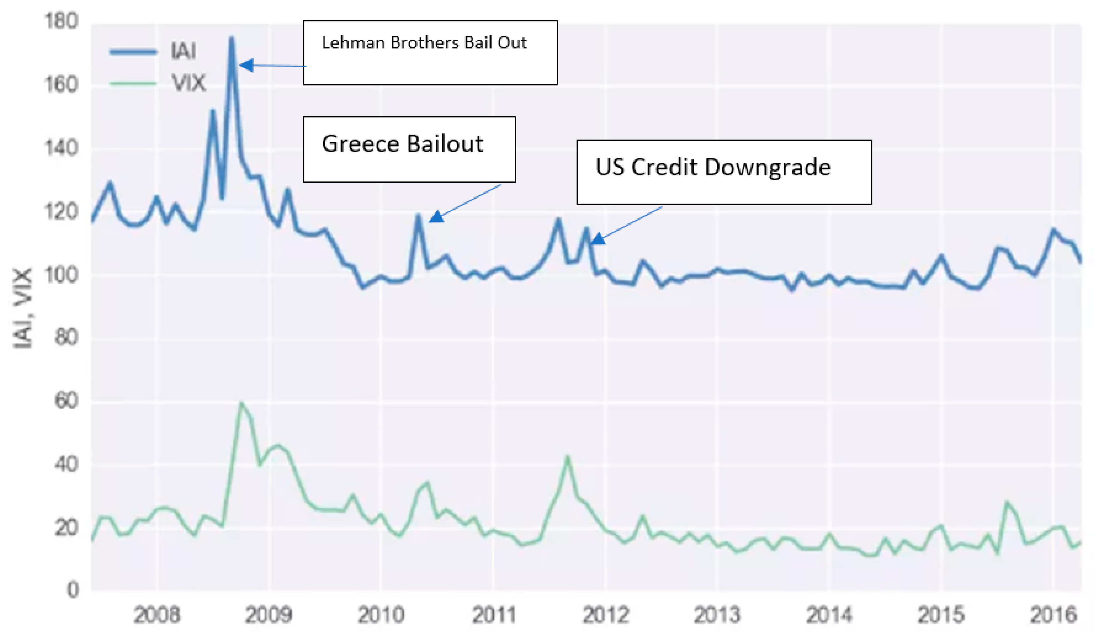
There have been other approaches to assessing market sentiments and fear. Investopedia developed an Anxiety Index (IAI), which is also designed to gauge investor sentiment based on the actions of thirty million Investopedia readers globally. Unlike the VIX, it tracks investors’ and readers’ interest in twelve financial terms. The IAI and the VIX are remarkably similar in terms of measuring market jitters. Figure 2 shows that the two indices move in tandem and confirm that, while computed from different sources and by different methodologies, they reflect almost identical information regarding investor sentiment.

This study examines the association of the SPRB with the VIX. The objective is to determine whether the regional bank equity index reacts similarly to the VIX as does the S&P 500. The findings of this investigation may be useful for bank regulators, policy makers, and investors interested in this sector. The findings may provide useful information for the valuation of implied volatility-based derivatives, hedging strategies based on the VIX fluctuations.

The interest in the VIX and its content have resulted in many research papers (see Sarwar 2012a, 2012b; Fleming et al. 1995). According to Adrangi et al. (2019), many of these papers are based on regression analysis and some have overlooked problems that may result in spurious and unreliable findings.

Evidence in the market shows that the relationship between the VIX and the S&P 500 and the SPRB is not consistently negative. There have been many periods were the VIX predictions and market movements have diverged. In other words, there may be structural breaks in the implied volatility and market performance relationship.

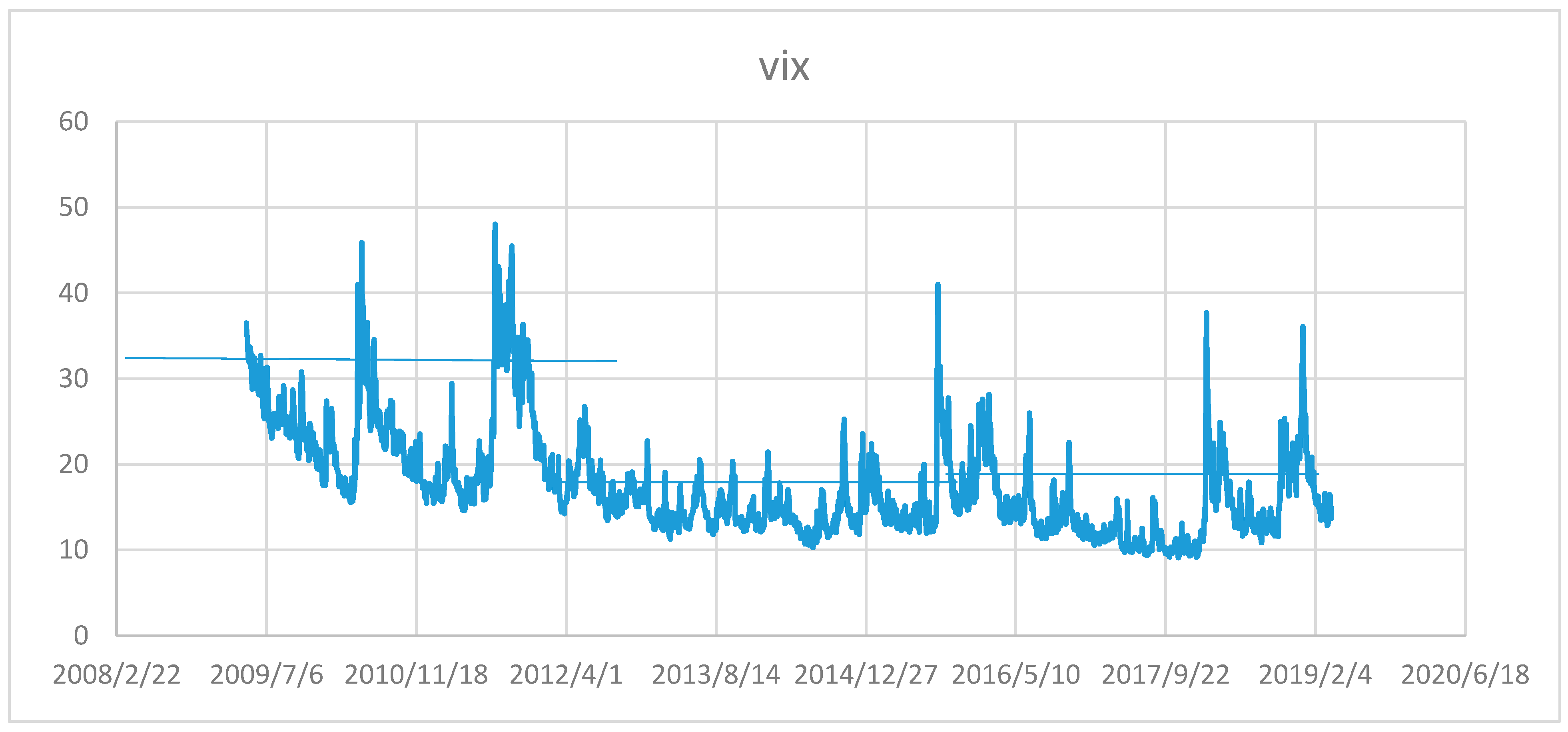
In this study, we suggest methodologies that deal with structural breaks in the data. We test for structural breaks in the VIX graphically (see Figure 3) and statistically. This approach allows us to deploy methodologies that may be robust in the presence of structural breaks.

Our empirical findings show an association between the VIX and SPRB in the time and frequency domains. To account for other variables that may be related to variations in the SPRB, we also included capacity utilization, consumer confidence, and the 10-year treasury bill rate. Our Kalman filter and quantile regression estimates capture the dynamic effects of structural breaks and possible extreme volatility on the model coefficients. The estimation results by both methodologies show a negative and statistically significant association between the VIX and SPRB.

The remainder of the paper is organized as follows. Section 2 offers a brief review of the relevant literature. The data are explained in Section 3. The methodology of the paper is the subject of Section 4. Section 5 consists of the analysis of the empirical findings. The last section is devoted to the summary and conclusions.

2. Review of the Relevant Literature

Research papers examine the content of the VIX and its role in predicting volatility in equity markets. Among this group of papers are Blair et al. (2010), Bekaert and Hoerova (2014), Giot (2005), and Corrado and Miller (2005), among others. The findings of these papers indicate that the VIX and its variations, such as the VXN (based on the NASDAQ 100 implied volatility) and VXO (implied volatility of the S&P 100 index) are useful predictors of future volatility in equity markets.

Many studies have investigated the association between the U.S. equity market and the VIX (Fleming et al. 1995; Whaley 2000, 2009; Connolly et al. 2005; Giot 2005, among others). These studies almost unanimously find a substantial negative contemporaneous association between the VIX and U.S. equity returns. In a related study, Durand et al. (2011) shows that the market risk and value premiums in the Fama and French (1993) three-factor model respond to changes in the VIX.

Several papers in the last decade have researched the association between the VIX and other asset classes. Notable among them are papers that investigate fixed-income securities, commodities, and foreign currencies, among others (see Badshah et al. 2013; Boscaljon and Clark 2013; Jubinski and Lipton 2013; Sari et al. 2011).

A number of research papers extend this investigation to cross-market associations of the VIX and equity markets of Europe, BRICS, Latin American equity markets, and other emerging markets. Notable among them are papers by Sarwar and Khan (2017), Smales (2016), Sarwar (2012a, 2012b), Neffelli and Resta (2018), and Ang et al. (2006). Skiadopoulos (2004) investigates implied volatility indices and their properties and relationships with equity markets in Greece. Frijns et al. (2010) investigates similar relationships in the Australian equity market.

Many of these studies unequivocally confirm the negative association between equity market returns and the VIX. These findings are not surprising as the co-movement among equity markets in the United States and the rest of the world has been well-documented (Rapach et al. 2013; Yunus 2013). It is reasonable to expect that the negative association of the VIX with U.S. equities will spill into other markets that show co-movement with the U.S. equity markets.

Papers that examine the association of the VIX with performance indices of specific sectors of the U.S. economy are much fewer. The implied assumption may be that sector performance is consistent with the U.S. equity market at large. However, this assumption may not be taken as an article of faith. In this paper, we investigate the association of the VIX with the SPRB.

The importance of banks in economic development is self-evident. Research on the possible role of the VIX in this sector, and the association of the VIX with the S&P 500 banking indices is nonexistent, presenting an unusual gap in the literature. The focus of this paper is on regional banks because they have a different business model than large international and money center banks in the United States. Historically, their business has been centered on deposits and loans in their communities. These banks are not typically involved in investment banking or trading. Their role has been significant in regional economic growth by providing loans to consumers and small businesses.

The financial crisis of 2008 brought changes to the banking industry, which affected large and regional banks alike. Furthermore, it showed the vulnerability of regional banks to economic shocks. Regional banks depend on deposits from the communities in which they operate. Roughly 70–80% of their liabilities are deposits from their communities. On the assets side, the loans to consumers and businesses are typically on par with their deposits. The prominent role of deposits in offering loans, and the lack of diversified sources of funding for loans, exposed regional banks to economic shocks far more than international banks. Therefore, economic shocks that adversely affect regional banks’ main source of loans—deposits by regional customers—impose serious constraints on the ability of regional banks to provide needed capital for economic development and regional capital investments. These constraints on their source of capital contributes to a slow recovery from financial shocks, similar to the 2008 crisis.

The same constraints that limit the ability of regional banks to provide loans, similarly, have adverse effects on their revenue. For instance, historically, regional banks have earned roughly 2% on their assets. However, during and after the financial crisis in 2008, these returns were negative, threatening the survival of many regional banks. The returns on assets slowly turned positive around 2014. Currently, the return on assets of regional banks hovers around 1.3%, a far cry from the robust levels before the financial crisis. In the post financial crisis era, new regulations and changes to the financial structure of regional banks have altered their business practices and ability to maintain financial profitability and viability. The SPRB reflects the general market sentiments regarding regional bank performance and relevance. Examining the performance of regional banks since 2009 could offer an understanding of the reaction of this sector to economic and financial shocks. One way of accomplishing this goal is to test the association of the regional bank index with the VIX.

3. Data

The daily data for this paper covers 30 April 2009 through 31 January 2019. The daily index values of the SPRB and the VIX are taken from the Bloomberg database. Our model includes variables that capture the real economic activity, interest rates, and consumer sentiment in the economy. We introduce capacity utilization to account for the real economic activity. This series is available on a monthly basis, follows the real GDP, and reflects the business cycle. The University of Michigan consumer confidence index is also available on a monthly basis, and it is widely reported to measure the movement in consumer confidence. Given that consumer spending accounts for roughly 70% of the GDP in the United States, it may also be associated with consumer loans for expenditures on durable goods. To convert the monthly series to a daily series, we utilize a natural cubic spline that connects the two consecutive monthly values. The cubic interpolation method is dynamic, and the interpolated daily series dynamically changes as the monthly values in the series change. The daily data closely tracks the monthly observations. This methodology is similar to the mixed interval data sampling (MIDAS) method. Once the daily data are derived, the dates are matched to the existing dates for the SPRB daily values.

The 10-year intermediate U.S. treasury bond is included in the model as the bellwether rate that gauges the trends in the treasury bond markets. The 10-year bond rates reflect many other important financial trends and sentiments, such as mortgage rates and investor confidence. At high levels of investor confidence, the demand for the 10-year bond may decline, leading to price falling bond prices and rising yields. Conversely, its price rises and yields drop with sagging investor confidence. Including this variable may capture the fluctuations in regional bank revenue and their stock prices. Including these variables will account for the movement of the SPRB because of macroeconomic conditions in the economy.

4. Methodology

We begin with a regression model that summarizes the relationship between the dependent variable SPRB and explanatory variables, consumer confidence (CC), capacity utilization (CU), rates on the 10-year US treasury bonds (tr_10), and the VIX. Equation (1) is the implicit regression model which is the mainstay of the empirical investigation in this paper.

SRRB = f(CC, CU, tr_10, VIX)

(1)

Prior to testing the association of the VIX with SPRB, we examine VIX for possible structural breaks. If we find breaks in the series, appropriate methodologies will be deployed to capture the effects of the breaks in data on the relationship among the variables. Furthermore, it is necessary to test each time series for stationarity. In the following, we briefly explain the methodology used in the paper.

4.1. Structural Breaks and Stationarity

We apply Bai and Perron (2003) test of structural breaks. We also examine the stationarity of the series under study by deploying augmented Dickey Fuller (ADF, Dickey and Fuller (1979)), Phillips–Perron (PP, Phillips and Perron (1988), and KPPS (Kwiatkowski et al. (1992)) tests. Tests of structural breaks and stationary are well known and covered widely in the literature and we will not repeat them in this section in the interest of brevity.

4.2. Spectral Analysis and Co-Spectral Analysis

As shown in the literature (Box and Jenkins 1976; Chatfield 1989), the behavior of most variables may be examined both in time or frequency domains. In this paper, we deploy both types of analyses using Kalman filter and quantile regressions in the time domain, and spectral/co-spectral analyses in the frequency domain. Examining returns in the frequency domain complements the analysis in the time domain, especially considering that nonlinearities often complicate econometric modeling.

Adrangi et al. (2020) offer a concise explanation of spectral and co-spectral analysis. We present a brief summary of the methodology and refer interested readers to Chatfield (1989) and Adrangi et al. (2020). Spectral analysis is based on expressing a stationary times series in terms sine and cosine waves of various frequencies. To estimate the amplitude of the sinusoidal components of a time series, periodograms (sample spectral density function) are defined. The sample spectrum is the Fourier cosine transformation of the estimation of the sample autocovariance function, and is written as follows,

$$I(f)=2\{{\sigma }_0+2{\displaystyle \sum _{F=1}^{N-1}{\sigma }_F\cos 2\pi fF\}}, 0 \le f \le 1/2.$$

(2)

The sample power spectrum is analogous to the probability density function in the continuous domain or a histogram in discrete domain. Converting variance and autocovariances to auotcorrelation coefficients, we obtain the following smooth estimate of the spectrum, I(f),

$$\widehat{P}(f)=2\{1+2{\displaystyle \sum _{F=1}^{N-1}{\lambda }_F^{}{\rho }_F\cos 2\pi fF\}}, 0 \le f \le 1/2.$$

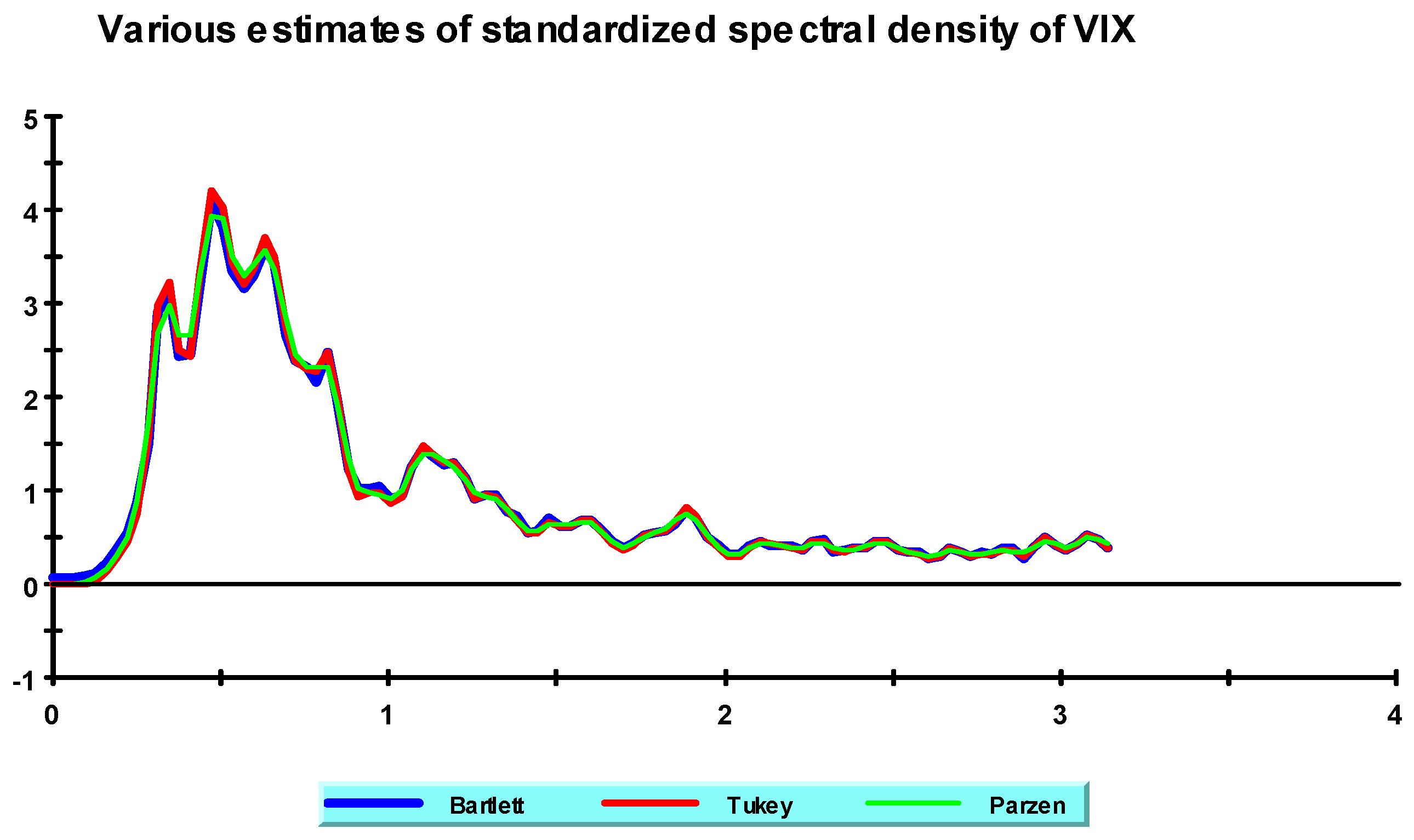
The variables λ_F are known as “lag window.” In the estimation process, one increases “the bandwidth” of the estimate to derive smooth estimates of the spectrum. We will estimate the individual spectrums for various time series utilizing three different lag windows, i.e., Bartlett, Tukey, and Parzen.

The standardized spectrum may be written as,

$$\widehat{P}({\theta }_j)= 2\{1+2{\displaystyle \sum _{F=1}^{N-1}{\lambda }_F{\rho }_F\cos 2F{\theta }_j\}},$$

(3)

where θ_j = jπ/m and j = 0, 1, 2 …… m and m is the window size and ρ_F is the autocorrelation coefficient of order F.

Examining co-spectral densities may shed further light on the association between two time series in the frequency domain. However, cross-spectral density is often complex-valued and is not directly informative. In our analysis, we focus on the “phase lead” and “coherence squared.” The phase lead measures the fraction of cycle that one series leads the other or lags behind in each frequency. The coherence squared measures the fraction of the variance of a time series which is explained by the variance in other series, in each frequency.

4.3. Kalman Filter

Structural breaks in the VIX and possible dynamic evolution of the association of the SPRB and explanatory variables of the model, requires estimation techniques that are suited to capture the model parameters in a dynamic manner. Ordinary least squares (OLS) estimation method may not be the best methodology in this situation. Kalman filter offers an alternative to OLS that is capable of taking into account dynamic development of the model.

The dynamic path of the n × 1vector y_t in a linear state—space can be formulated by the system of equations

$$y_t={\varphi }_t+{\alpha }_t{X}_t,$$

(4)

$${\alpha }_{t-1}={\gamma }_i+T_i{\alpha }_t+{\upsilon }_t,$$

(5)

where y_t, SPRB in this study, is assumed to follow a first-order vector autoregression, ${\alpha }_t$ is an n × 1vector of unobserved state variables, ${\varphi }_t,X_t,{\gamma }_t,T_t$, are conformable vectors and matrices, and $u_t$ and ${\upsilon }_t$ are vectors of Gaussian innovations with zero mean, zero autocovariance, and the contemporaneous covariance matrix:

$$\Lambda =\left(\begin{array}{cc}{\Phi }_t& {\Gamma }_t\\ {\Gamma }_t^{\prime }& {\Theta }_t\end{array}\right).$$

(6)

${\Phi }_t$ and ${\Theta }_t$ are n × n and m × m symmetric matrices of variances, and ${\Gamma }_t$ is an n×m matrix of covariances, respectively.

The first set of Equation (4) are the “signal” or “observation” equations and the second set (5), the “state” or “transition” equations.

The updating equation is for the states in period t + 1, given the errors specified in period t. This timing convention, which follows Koopman et al. (1999), has important implications for the interpretation of correlations between errors in the signal and state equations ${\Gamma }_t$.

We generalize the specification above, where ${\varphi }_t,x_t,{\gamma }_t,T_t$, ${\Phi }_t$, ${\Theta }_t$, ${\Gamma }_t$ are conformable matrices and vectors that depend on observable explanatory variables x and unobservable parameters Ω.

Given information available at time t − 1, the one-step ahead conditional mean and variance of the states ${\alpha }_t$ are

α_t|t−1 = E_t−1 (α_t)
V_t|t−1 = E_t−1 [(α_t − α_t|t−1) (α_t − α_t|t−1)’].

(7)

The equation set (7) is used to compute the minimum one-step ahead estimate of the mean squared error for y_t by

y_t|t−1 = E_t−1(y_t) = E(y_t|αt|τ).

(8)

The one-step ahead prediction error is given by

$${\widehat{\nu }}_t={\nu }_{t|t-1}\equiv y_t-y_{t|t-1},$$

(9)

and the prediction error variance is defined as

$${{\sigma }^2}_{t|t-1} = \mathrm{VAR}\left(y_{t|t-1}\right) = X_t V_{t|t-1} {X^{\prime }}_t + {\Phi }_t.$$

(10)

Space/state models can be estimated by Kalman filter. This methodology recursively updates the state mean and variance as new information becomes available. For instance, with initial values of the state mean and covariance, system matrices, and observations on y_t, the Kalman filter computes one-step ahead estimates of the state variable α_t|t−1 and the associated mean square error matrix, the contemporaneous or filtered state mean and variance, α_t and V_t, and the one-step ahead prediction, prediction error, and prediction error variance, in Equation (8) through (10), respectively.

For instance, if we have the time series up to time period S, we may use this information to form expectations up to S, which is known as fixed-interval smoothing.

Smoothing uses all of the information in the sample to provide smoothed estimates of the states, ${\widehat{\alpha }}_t={\alpha }_t{|}_S=E_S({\alpha }_t)$, and smoothed estimates of the state variances, $S{V}_t=Va{r}_S({\alpha }_t)$. The matrix SV_t, may also be interpreted as the MSE of the smoothed state estimate ${\widehat{\alpha }}_t$.

In a similar one-step process, we may use the smoothed values to form smoothed estimates of the signal variables

$$y_{t|t-1} \equiv E_{t-1}({y_t}_{|}{\widehat{\alpha }}_t) ={\varphi }_t+{\widehat{\alpha }}_t{x}_t,$$

and to compute the variance of the smoothed signal estimates

$$G_t \equiv Var(y_{t|S}) = X_t S{V}_t {X^{\prime }}_t.$$

The smoothed disturbance estimates

$${\widehat{\upsilon }}_t={\upsilon }_t{|}_S\equiv E_S({\widehat{\upsilon }}_t),$$

and ${\widehat{\xi }}_t={\xi }_t{|}_S\equiv E_S({\widehat{\xi }}_t)$ and a corresponding smoothed disturbance variance matrix are also derived as

$${\Sigma }_t=Va{r}_s\left(\begin{array}{l}{\upsilon }_t\\ {\xi }_t\end{array}\right).$$

Deploying the Kalman filter and the fixed-interval smoother requires substituting estimates of the unknown elements in the system matrices. Under the assumption that the $\widehat{\xi }$ and ${\widehat{\upsilon }}_t$ are Gaussian, the sample log likelihood

$$LNL(\Psi )=-n/2TLn2\pi -1/2{\displaystyle \sum _{t}Ln|{\sigma }_t^2}(\Psi )|-1/2{\displaystyle \sum _t}{\overline{\xi }}^{\prime }(\Psi ){\sigma }_t^2{(\Psi )}^{-1}\overline{\xi }(\Psi ),$$

may be evaluated using the Kalman filter. Using numeric derivatives, one maximizes the above likelihood function with respect to the unknown model parameters and obtains the estimates of these parameters.

4.4. Quantile Regression

The extreme movements in VIX and its structural breaks, potentially have asymmetric effects on the SPRB responses. Market participants and investors are not only sensitive to the average impact of VIX on SPRB (shown by VARs and OLS regressions), they are also interested in the impact of extreme up and down movements of VIX and the association of these movements with SPRB. Structural breaks may be one source of extreme fluctuations in VIX.

Quantile regressions (QR) are well designed to accommodate the asymmetric dependence between dependent and explanatory variables. QR models are non-linear models (see e.g., Galvao et al. 2020) that are robust in the presence of extreme events and asymmetric dependence when the assumption of linearity may not be appropriate (see Geraci 2019; Yu et al. 2003). They are superior to OLS estimates because they allow coefficient estimates to vary with the distribution of the dependent variable, thus, accurately modeling the relationship between the explanatory variables and the dependent variable. A brief explanation of QR is presented below.

Suppose that we have a random variable Y (SPRB in this paper) with probability distribution function

F(y) = Prob(Y ≤ y),

so that for 0 < τ < 1, the τth quantile of Y may be defined as the smallest y satisfying

$$\begin{gathered} F(y)\ge \tau : \\ Q(\tau )=\inf \left\{y:F(y)\ge \tau \right\}. \end{gathered}$$

The empirical distribution function is given by

$$F_n(y)={\displaystyle \sum _s^{}l(Y_i\le y)},$$

where l(.) is a binary function that takes the value 1 if $Y_i\le y$ is true and 0 otherwise. The resulting empirical quantile is given by

$$Q_n(\tau )=\inf \left\{y:F(y)\ge \tau \right\}.$$

Alternatively, it may be expressed as an optimization problem as

$$Q_n(\tau )=\arg \min \left\{{\displaystyle \sum _i{\rho }_{\tau }(Y_i-\omega )}\right\},$$

where ${\rho }_{\tau }(w)=w(\tau -1(w<0))$, which, asymmetrically assigns weights to positive and negative values in the estimation process.

The extension of this methodology that allows for regressors X is the quantile regression. We assume a linear specification for the conditional quantile of the dependent variable SPRB given values for the vector of explanatory variables X such that

$$Q(\tau |X_i,\beta (\tau ))=X_i^{\prime }\beta (\tau ),$$

where $\beta (\tau )$ is the vector of coefficients associated with the $\tau$th quantile.

Then the conditional quantile regression estimator can be shown to be

$${\beta }_n(\tau )=\arg {\min }_{\beta (\tau )}\left\{{\displaystyle \sum _i\rho (\tau Y_i-X_i^{\prime }\beta (\tau )}\right\}.$$

The quantile regression estimator is derived as the solution to a linear programming problem. We use a modified version of the Koenker and D’Orey (1987) version of the Barrodale and Roberts (1973) simplex algorithm.

Under mild regularity conditions, quantile regression coefficients may be shown to be asymptotically normally distributed (see Koenker and Ng (2005)) with the asymptotic covariance matrix depending on the model assumptions. The coefficient covariance matrices in quantile regression analysis are obtained from estimated nuisance quantities.

In this paper, we relax the assumption that the quantile density function does not depend on X. The asymptotic distribution of $\sqrt{n(\widehat{\beta }(\tau )-\beta (\tau )}$, under the identically and not independently distributed (i.n.i.d.) assumption is expressed in the Huber sandwich form (see, among others, Hendricks and Koenker 1992)

$$\tau (1-\tau )H{(\tau )}^{-1}JH{(\tau )}^{-1},$$

where,

$$J={\lim }_{n\to \infty }({\displaystyle \sum _i{X}_i{X}_i^{\prime }/n}),$$

and $H(\tau )={\lim }_{n\to \infty }({\displaystyle \sum _i{X}_i{X}_i^{\prime }{f}_i(q_i(\tau ))/n})$, and f_i(q_i(τ)) is the conditional density function of the response, evaluated at the τth conditional quantile for individual i. We deploy the Powell (1984) kernel method based on residuals of the estimated model.

The Powell (1984) kernel approach computes a kernel density estimator using the residuals of the original fitted model

$$\widehat{H}=1/n{\displaystyle \sum _{}{b}_n^{-1}}K(\vartheta (\tau )/b_n{X}_i{X}_i^{\prime },$$

where K is a kernel function that integrates to 1, and b_n is a kernel bandwidth. For bandwidth specification, we employ a method suggested by Hall and Sheather (1988) and a kernel bandwidth suggested by Koenker and Ng (2005). Koenker and Machado (1999) define a pseudo R-squared for the goodness-of-fit statistic for quantile regression that is analogous to the R squared from conventional regression analysis.

5. Empirical Findings

5.1. Structural Breaks and Stationarity

The Bai–Perron test signals three structural breaks that occur around 20 January 2012, 19 December 2014, and 7 July 2016. The first break appears to coincide with developments in the oil markets. A tightening of the oil supply by Saudi Arabia and the United States entering the shale oil market were significant economic triggers. Hurricane Sandy inflicted huge costs on the U.S. economy and temporarily disrupted the supply chain while threatening economic growth in the United States. Political crises in Iraq and Syria were sources of uncertainty in the Middle East and spanned global economies.

Th second break appears to coincide with several political and economic upheavals. First, the weak economic condition in the European Union (EU), which is the largest world economy. Second, the political crisis between Russia and the Ukraine, and the economic fallout from this conflict had an adverse effect on the geopolitical and economic woes in Europe. Third, the continuing problems in Iraq and Syria added to uncertainty in the global economies. The last break could have been because of Britain’s vote to leave the EU, a populist outburst that could steer its economy into uncharted economic waters. Markets dropped, and the British pound weakened. Furthermore, China’s economy was showing signs of strain and was slowing down around the same time. Equity markets in the United States were down by about 15%, mostly because of the problems experienced by China. Oil prices hit levels below $30 a barrel.

Examining the graphs of the SPRB, consumer confidence and capacity utilization suggest that the prices show mean and covariance nonstationary. However, the VIX series, while showing structural breaks, may be stationary. The graphic evidence (not presented for the purpose of brevity) of nonstationary calls for formal statistical tests. We provide the statistical evidence of the behavior of these series in

Table 1. Break points, diagnostics, and summary 30 April 2009–31 January 2019.

Panel A: Bai-Perron Test of Structural Breaks
Break Test	Scaled F-Statistic		Critical Value *	Dates
0 vs. 1 a	1701.59		8.58	20 January 2012
1 vs. 2 a	68.96		10.13	10 December 2014
2 vs. 3 a	42.26		11.14	7 July 2016
3 vs. 4	0.00		11.83
Panel B: Levels
		CC	CU	SPRB	VIX
ADF		−1.318	−4.613 a	−1.211	−6.452 a
PP		−1.766	−4.414 a	−1.175	−6.310 a
KPPS		5.412 a	2.349 a	5.453 a	2.517 a
Panel C: Hodrick-Prescott Detrended Series
ADF		−19.51 a	−17.748 a	−19.878 a	−20.411 a
PP		−19.036 a	−19.332 a	−52.965 a	−56.499 a
KPPS		0.003	0.033	0.029	0.027
Panel D: Summary Descriptive Statistics for Model Variables. All Variables Are in Level
Mean	83.421		76.100	1182.885	17.661
Stand Dev	11.428		2.630	396.484	6.136
Skewness	−0.204		−1.691	0.514	1.351
Kurtosis	1.881		6.018	2.182	4.967
J-B	145.237 a		2102.665 a	176.558 a	1143.153 a

Notes: * Bai and Perron (2003) (Econometric Journal), critical values. The null hypotheses for ADF and PP tests is that a series is nonstationary. KPSS tests include an intercept in the test regression and test the null that the series is trend-stationary. Significance of KPPS indicates nonstationary. ^a represent significance at 1percent level.

.

Table 1 presents the summary statistics of the series under study. Some of the time series under study are found to be nonstationary, employing the augmented Dickey Fuller (ADF), Phillips–Perron, and KPPS statistics. While the capacity utilization and the VIX are stationary for two of the tests, the remaining series are not stationary. However, application of the Hodrick–Prescott (HP) filter produced a series that is statistically stationary by every test as shown in Table 1, Panel B. In the remainder of our empirical investigation, we will use the stationary series produced by the HP filter or the first differences of the series whenever the methodology requires the variables to be stationary.

5.2. Spectral and Co-Spectral Analysis

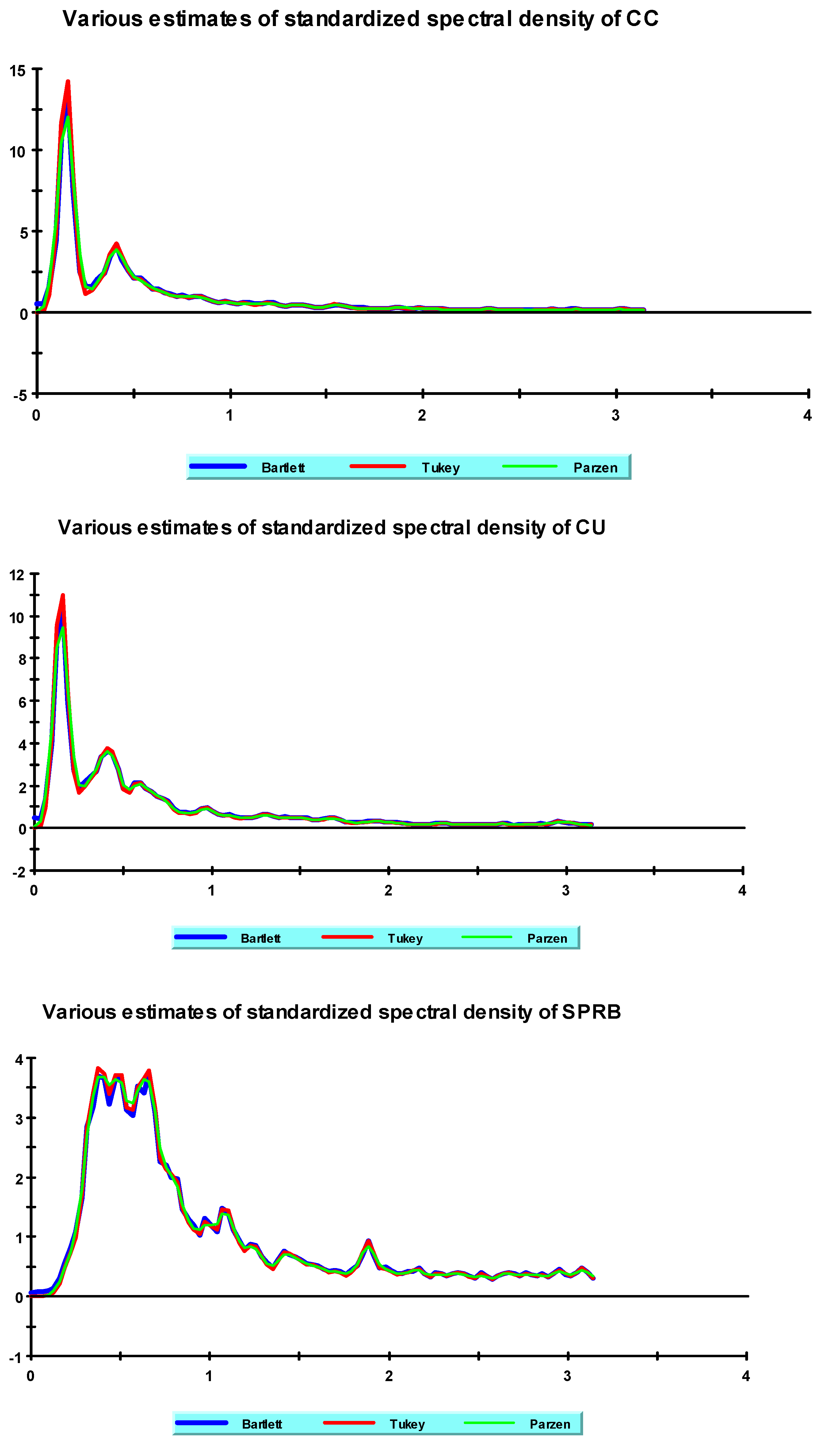
Examining the standardized spectral densities for the four series in Figure 4 shows that the majority of the variations in the four time series are concentrated in low frequencies. This pattern of variation may be a sign of a low-frequency response to the VIX by the SPRB, which may not be detectable in a high-frequency time series, such as intraday data. In other words, testing the daily data may properly capture the responses of SPRB to the VIX volatility. However, structural breaks may require methodologies that account for breaks and produce time-varying estimates.

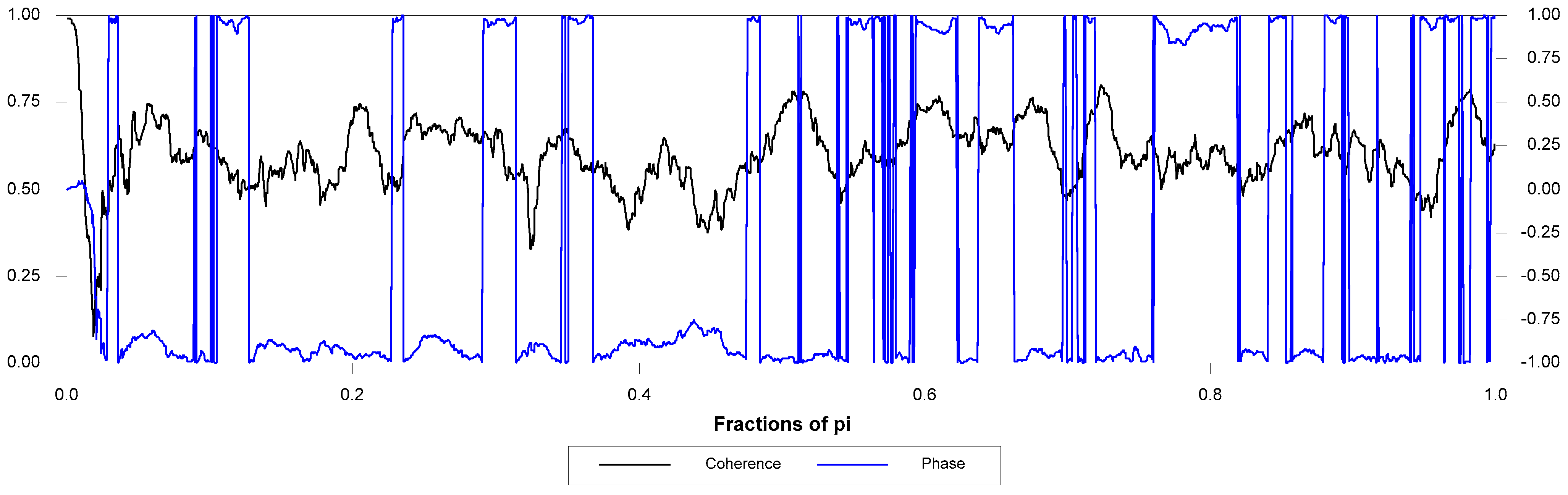
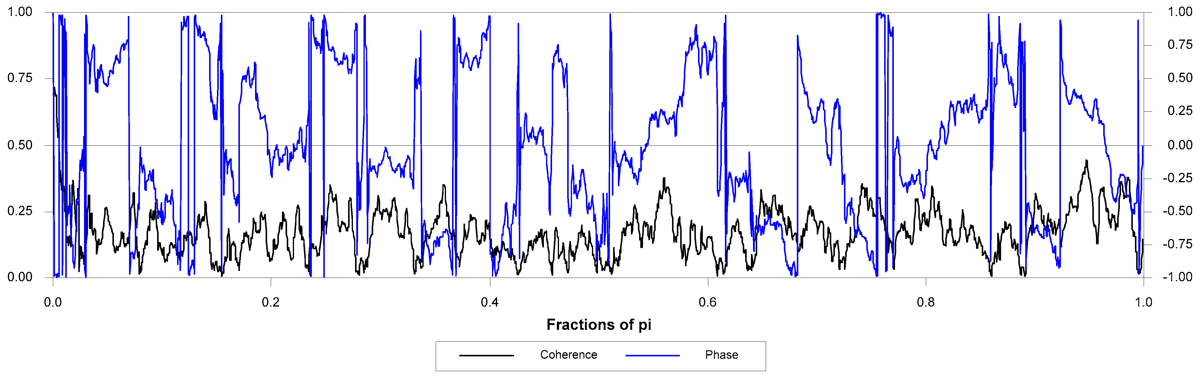
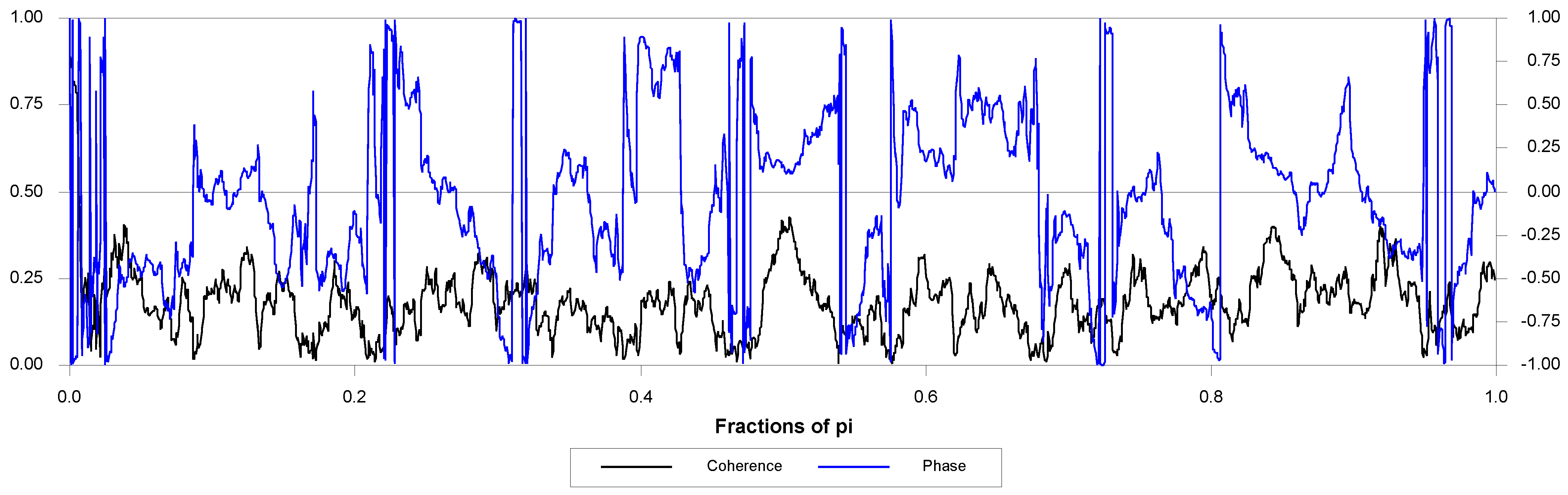
Based on the analysis of the spectral density function, we conclude that the four series under study may still be coherent in the frequency domain (i.e., move in tandem). To investigate this possibility, we analyzed co-spectral density functions between the SPRB and the remaining variables in the study. The cross-spectrum indicates how much linear information is transferred from one signal to the other and vice versa (i.e., the “burden” of the line transfer at each frequency). We will focus on “coherence” and “phase” between two series or their representations in the frequency domain.

Coherence is a measure of the degree of a relationship, as a function of frequency, between two time series. It describes the correlation (or predictable relationship) between waves at different frequencies or moments in time. Alternatively, the coherence indicates how much linear information in one signal is explained by the other signal. The coherence of a linear system of a relationship reveals the fraction in the volatility of movements in variable y that is because of the variable x at a frequency. It may be used to estimate the association or even causality between the two signals.

If the coherence (C_xy) is between zero and one, it could be an indication of the presence of random disturbances, which are common in markets. Alternatively, it could be showing that the assumed function relating x(t) and y(t) is not linear. Another possibility may be that y(t) is dependent on x(t) as well as other input. If the coherence is equal to zero, it is an indication that x(t) and y(t) are perfectly unrelated.

Figure 5, Figure 6 and Figure 7 present the phase lead and coherence between SPRB and each of the time series under study. For instance, in the 0–1 frequency (π), by more than fifty percent of the cycle, the VIX leads the SPRB. The same is roughly true in the case of consumer confidence and capacity utilization. In almost all of the fractions of the frequency domain (π), CC and CU appear to lead the SPRB series by roughly 50% of a cycle. One may interpret this observation as a weaker lead/lag association between SPRB and the latter two time series variables. It is possible that SPRB is contemporaneously associated with CC and CU.

In regard to the graph of coherence, one concludes that in all frequencies (low to high), a high percentage of variation in the SPRB appears to be explained by the variations in the VIX, consumer confidence, and capacity utilization. These observations strongly support the hypothesis that variations in the SPRB are associated with the other three variables in the sample. The findings of the phase lead and coherence squared also suggest that the VIX may contain information not included in the consumer confidence, capacity utilization, or SPRB. The arrival of the information may initially occur in the VIX. It is important to note that the low-frequency spectral density in a series may resemble a long-term trend in the time series presentation of the series. In this context, the coherence between the SRB and the three series may point to a correlation, or even a causality, between the three variables—the CC, CU, and VIX variables and the VIX in the time domain.

Mathematically, spectral analysis is equivalent to the results of the covariance in the time domain, and the spectral density function serves the same purpose as histograms in the time domain. We use the information gleaned from the spectral and the cross spectral investigation and estimate the Kalman filter and quantile regressions that successfully capture the transitions of the association among the variables across the structural breaks.

5.3. Kalman Filter Estimation

The Kalman filter estimation results are summarized in

Table 2. Kalman filter estimation of Equation (1).

SPRB	C1	CC	CU	tr_10	VIX	LL
	23.162	5.068 a	16.327 a	−3.982	−6.452 a	−9964.262
	(31.173)	(1.693)	(5.373)	(5.754)	(0.171)
state sv1 = sv1(−1)
state sv2 = α×sv2(−1) + β×sv3(−1) + [var = exp(c(4))]
state sv3 = sv2(−1)

Significance indicates nonstationary. ^a represents significance at 1 percent level.

. The coefficient of VIX is time varying and is assumed to be a state variable. That allows the estimated coefficient to be updated through the estimation process in a dynamic manner. The Kalman filter estimation shows that consumer confidence and capacity utilization contribute to the SPRB positively and are statistically significant. This finding is plausible as consumer confidence is expected to be correlated with consumption expenditures. Consumption expenditure in the United States accounts for roughly 70% of the GDP. Therefore, stable levels of consumer spending would contribute to GDP growth. This, in turn, contributes to banking activities, such as consumer loans, mortgages, and auto loans. Regional banks will benefit from these activities.

Capacity utilization levels also have a similar effect on regional banks as they support employment and consumer spending. Oddly, the bellwether 10-year treasury bond rates do not show a significant bearing on the regional bank index in this sample. The coefficient of the VIX, which is a state variable, is negative and statistically significant. This finding indicates that the increases in the fear index are associated with the declines in the regional bank equities and, thus, the regional bank index. This is consistent with our prior expectations. To examine the robustness of the Kalman filter results, we also estimate and report quantile regression estimation results in deciles of the SPRB as the dependent variable.

5.4. Quantile Regression Findings

In the interest of brevity, we only report the first, fifth (median), and ninth quantile results. As shown in

Table 3. Quantile regression estimation of Equation (1).

D(SPRB)	1st Q	C	DCC	DCU	DVIX	Ps_R2	Quasi_LR
		−15.291 a	3.022	65.581 a	−6.636 a	0.215	410.032 a
		(0.629)	(3.422)	(26.297)	(0.459)
D(SPRB)	5th Q
		0.107	3.349 a	32.492 b	−6.118 a	0.205	956.007 a
		(0.304)	(1.325)	(15.985)	(0.294)
D(SPRB)	9th Q
		16.508 a	2.926	−14.983	−6.256 a	0.171	341.955 a
		(0.500)	(3.507)	(30.100)	(0.168)
D(SPRB)	OLS	0.230	5.158 a	19.421	−6.245 a	0.350	440.403 a
		(0.290)	(1.501)	(13.996)	(0.172)

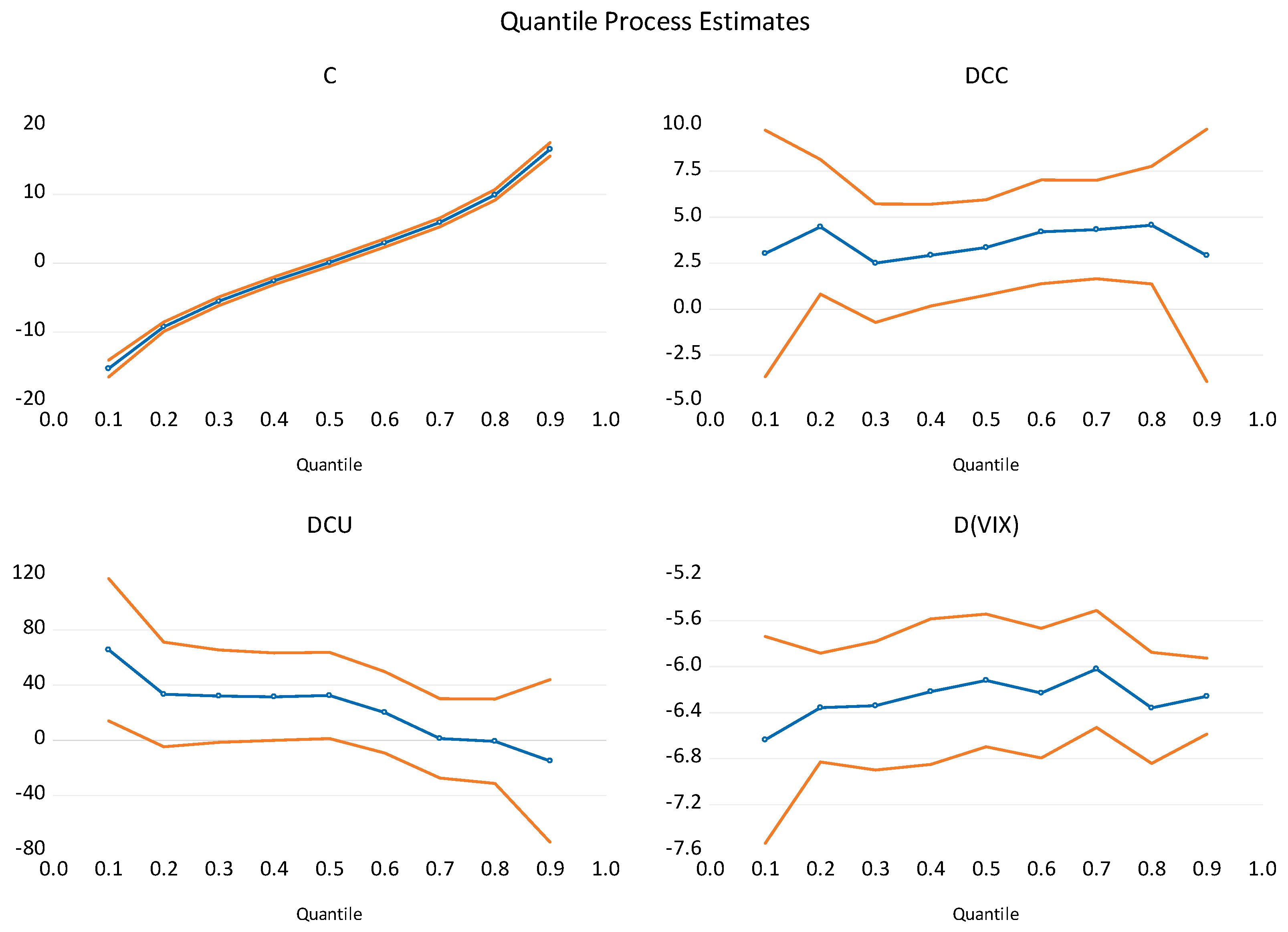
Notes: ^a, ^b represent significance at 1, 5, percent levels, respectively. The values of R-sq and likelihood ratio functions for the OLS estimates and pseudo R-sq and quasi-likelihood ratio functions are in the last two columns. Huber sandwich standard errors and covariances. Method of Epanechnikov kernel, and Hall–Sheather residuals bandwidth (bw = 0.025648).

, the three quantile regression estimates are qualitatively similar. Regressions are estimated in the first differences of all of the variables to induce and ensure stationarity with a different approach than the HP methodology. The 10-year bond rates are dropped because they were statistically insignificant in the Kalman filter methodology. The most important observation is that the association between the VIX and the SPRB remains statistically significant and negative. Furthermore, the magnitude of the coefficient of the VIX is comparable to the estimates from the Kalman filter approach confirming the robustness of the coefficient estimate. The pseudo R-squared is roughly around 0.21; however, this observation is typical for quantile regression. The quasi likelihood ratio test indicates that the explanatory variables, collectively, are significantly associated with the SPRB. A comparison of the OLS estimates with various estimates at the reported quantiles confirms that the association between the VIX and SPRB is nearly stable, though the value of other coefficients and their statistical significance for the remaining model variables are not. This is a plausible observation and is possibly explained by the reaction of consumers and producers to the shifting economic climate as indicated by the VIX.

Figure 8 shows the estimated coefficients and their 95% confidence band over nine quantiles. While the coefficient estimates are fairly stable around the fiftieth quantile, at the tails of the distribution coefficient, the values show changes indicating that the association of the SPRB with explanatory variables at the extremes is influenced by structural breaks in the VIX.

6. Summary and Conclusions

The objective of this study is to examine the reaction of the SPRB to the variations in the U.S. fear index, VIX. Practitioners and academicians have been interested in the role of the VIX as a leading indicator of the volatility in equity markets. Regional banks have experienced economic difficulty during periods of financial volatility. However, they also play a significant role in the economic development of various regions in the United States. While the academic research presents a near unanimous negative relationship between the VIX and equity markets, this relationship has not been investigated for equities in many sectors of the economy.

Practitioners observe many periods of divergence between the VIX and equity indices, such as the S&P 500. The present study investigates the association of the VIX as a leading indicator of financial markets with the SPRB. The findings may provide information that could assist regional banks, regulators, and policy makers in coping with volatility in financial markets.

Our paper examines the daily data for the period of 2009 through 2019. We find three significant structural breaks in the VIX data during this period according to the Bai and Perron (2003) test. The breaks coincide with significant economic and political upheavals, such as the EU economic problems, disruptions in the crude oil market, and Brexit vote.

Our empirical findings show an association between the VIX and SPRB in the time and frequency domains. To account for other variables that may be related to variations in the SPRB, we also included capacity utilization, consumer confidence, and the 10-year treasury bill rate. Our Kalman filter and quantile regression estimates are designed to capture the dynamic effects of structural breaks and possible extreme volatility on the model coefficients. The estimation results by both methodologies show a negative and statistically significant association between the VIX and SPRB.

Regional banks and regulators may be able to monitor the fluctuations in the VIX as a signal that regional banks may face financial uncertainties. For instance, high readings of the VIX may be considered a signal that regional banks should take precautionary measures. Fund managers who are invested in this sector could also use this information to reposition their portfolios to reduce the risk exposure to regional banks.