Dimension Reduction via Penalized GLMs for Non-Gaussian Response: Application to Stock Market Volatility

Abstract

We fit U.S. stock market volatilities on macroeconomic and financial market indicators and some industry level financial ratios. Stock market volatility is non-Gaussian distributed. It can be approximated by an inverse Gaussian (IG) distribution or it can be transformed by Box–Cox transformation to a Gaussian distribution. Hence, we used a Box–Cox transformed Gaussian LASSO model and an IG GLM LASSO model as dimension reduction techniques and we attempted to identify some common indicators to help us forecast stock market volatility. Via simulation, we validated the use of four models, i.e., a univariate Box–Cox transformation Gaussian LASSO model, a three-phase iterative grid search Box–Cox transformation Gaussian LASSO model, and both canonical link and optimal link IG GLM LASSO models. The latter two models assume an approximately IG distributed response. Using these four models in an empirical study, we identified three macroeconomic indicators that could help us forecast stock market volatility. These are the credit spread between the U.S. Aaa corporate bond yield and the 10-year treasury yield, the total outstanding non-revolving consumer credit, and the total outstanding non-financial corporate bonds.

1. Introduction

“We are drowning in information and starving for knowledge”; this statement by the American librarian Rutherford D. Roger (and others) was quoted by Hastie in his well-respected book Statistical Learning with Sparsity: The LASSO and Generalizations Hastie et al. (2015). Drowning in the big data environment, we statisticians are devoted to finding better ways of fitting effective distributions and identifying the few important indicators from an overwhelming number of potential indicators, so that we can gain knowledge of how to forecast the responses of interest and how to make the forecast interpretable as well.

Stock return volatility is pervasively watched in almost every industry sector. Examples are asset pricing, risk management, portfolio management, and market research. In this paper, we identify useful models for stock market volatility and use dimension reduction techniques to find some leading indicators, which can potentially be from macroeconomic indicators and stock market financial ratios.

Stock return/price volatility is defined as the standard deviation of the stock return/price. Quite often, financial industry workers use percent per annum as the unit of volatility. For example, a 20% volatility means a stock has a standard deviation of 20% for its yearly return. Volatility data are not random walk time series, and they display some apparent patterns, such as clustering and fat tails. Volatility clustering was first noted by Mandelbrot (1963), who pointed out that “large changes tend to be followed by large changes, of either sign, and small changes tend to be followed by small changes.”

Academic research, as well as financial industry studies, have focused on studying the strong persistence pattern of volatility time series data, described by volatility clustering and long memory. These two patterns are well captured by Generalized AutoRegressive Conditional Heteroskedasticity (GARCH) models and Fractionally Integrated Generalized AutoRegressive Conditionally Heteroskedastic (FIGARCH) models, respectively. The GARCH model, which was developed by Engle (1982) and Bollerslev (1986), is mainly used to model short time horizon (e.g., daily) time series. The GARCH model is intuitively built on an observation, that once the volatility surging momentum arises it will sustain for a while before it subsides. The GARCH model assumes stock returns conform to a Gaussian distribution conditional on its variance. Under normality and independence assumptions, the stock return can be described by a combined ARMA-GARCH model to capture the movement of the mean and the variance of stock return, respectively. The FIGARCH model was first introduced in Baillie et al. (1996) to capture the slow hyperbolic rate of decay of the influence of lagged squared innovations in the time series of the conditional variance of Deutsch Mark–U.S.Dollar exchange rates.

Both the GARCH and the FIGARCH models capture the volatility persistence pattern very well. However, there are two flaws in these models. Firstly, they do not do well in forecasting and secondly the distribution of the residuals is actually far from Gaussian. The Box–Cox transformation can be used to transform the non-Gaussian response variable into an approximately Gaussian distributed variable. At the same time, generalized linear model (GLMs) directly expand the distribution of the response variable to non-Gaussian exponential family distributions. Both methods can be used to deal with models whose response variable suffers from skewness and fat tails. In this paper, we combine the Box–Cox transformation framework with the least absolute shrinkage and selection operator (LASSO) method and the optimal link function for the inverse Gaussian (IG) distribution, again combined with LASSO, to capture macroeconomic conditions and stock market valuation factors that impact the stock market volatility significantly. In addition, the oracle property of LASSO models enabled us to forecast the stock market volatility surging momentum far further ahead with a low frequency quarterly data set. The paper is organized as follows. In the next section, we present a short description of the methods that we use. In the subsequent section, we provide the details about the implementation of these methods and apply them to simulated data. We then proceed with the empirical analysis using real world data, and finally we conclude. In the appendix we present some computational algorithms that were used in the analysis.

2. Methodology

2.1. Inverse Gaussian (IG) Distribution

To describe the process of stock returns, some non-Gaussian distributions have been used and were proven to be more appropriate than the Gaussian distribution. Stentoft (2006) gives a good review on the distributions that have been used to describe stock returns, such as the log-normal distribution in Clark (1973), the Student’s t-distribution in Bollerslev (1986), the generalized error distribution in Nelson (1991), the skewed Student’s t-distribution in Lambert and Laurent (2001), and the normal inverse Gaussian distribution in Jensen and Lunde (2001). Lars Stentoft further illustrates in his paper that the normal inverse Gaussian (NIG) distribution has an appealing property to describe the movement of stock returns, which property can be traced back to the mixing distribution hypothesis (see Clark (1973)): if returns are assumed to be normally distributed conditional on the variance, and if the conditional variance of the returns follows an inverse Gaussian (IG) distribution, then the unconditional distribution of the returns is a NIG distribution. Hence, we used the IG distribution to fit stock return volatility in this paper.

We used score tests and goodness of fit (GOF) tests, which were suggested by Ducharme (2001) and Desmond (2011), to rigorously check whether stock market volatility conforms to an IG distribution; see Appendix A for implementation details. The results in

Table 1. IG Goodness of Fit(GOF) test.

IG GOF Test	IG	${\mathit{Y}}_{\mathit{ig}}$	${\mathit{Y}}_{\mathit{ibc}}$	VXO	W5000	SP500	NASDAQ	Critical Value
								$95(\%)$	$99(\%)$
T2	−0.47	0.94	2.39	2.41	4.67	4.40	2.76	1.96	2.58
R3	0.74	2.83	6.81	5.31	14.98	11.33	13.11	7.38	10.60
V2	0.70	2.47	3.78	4.16	8.22	6.37	7.72	5.02	7.88
V3	0.04	0.36	3.03	1.15	6.76	4.96	5.39	5.02	7.88

T2 is the Desmond (2011) score test pivotal quantity, which is approximately standard normal; R3 is the Ducharme (2001) smooth test pivotal quantity, which conforms to the ${\chi }_2^2$ distribution; V2 and V3 are part of R3, which both conform to the ${\chi }_1^2$ distribution; they test the second and the third moment condition, respectively. IG data were generated directly via MATLAB random number generation function $random(.)$; $Y_{ig}$ and $Y_{ibc}$ data were generated from our simulation procedure. Further details are given in Section 3.1; VXO is implied stock volatility index; SP500, W5000, and NASDAQ are realized volatility of corresponding stock market indices.

show that we do not have sufficient evidence to reject the null hypothesis that the implied volatility (VXO implied SP100 index volatility) follows an IG distribution with Ducharme’s test. However, there is some evidence to reject the null hypothesis under certain confidence levels with both tests for the realized volatility, which are the Wilshire 5000 index realized volatility, the SP500 index realized volatility, and the NASDAQ index realized volatility. Hence, we focused our research on the implied volatility VXO index.

We used histograms, Quantile–Quantile (QQ) plots, and Probability–Probability (PP) plots to check the conformity of raw VXO index to IG distribution and the log transformed and Box–Cox transformed VXO index to Gaussian distribution. From these graphical checks, not shown here to preserve space, we find that the Box–Cox optimal transformed data conforms roughly to a Gaussian distribution and the raw scale data may be approximated by the IG distribution. This is also supported by additional Jarque–Bera tests.

Hence, we were comfortable using both the Gaussian LASSO model and IG GLM LASSO model to fit VXO implied volatility in this research.

2.2. Box–Cox Transformation

The Box–Cox transformation can be used to transform the non-Gaussian response variable into an approximately Gaussian distributed variable. In the context of a linear regression model, applying the Box–Cox transformation results in using a grid search to find the optimal parameter estimate that transforms the response variable into an approximate Gaussian form. We combine the Box–Cox model with the dimension reduction methodology of LASSO, a novel approach that introduces a number of challenges that go well beyond the individual characteristics of each method separately. We discuss the combined Box–Cox and LASSO model in detail in the next section.

2.3. Penalization Method

To identify important indicators from numerous potential indicators to help interpret and forecast the stock market volatility, LASSO models excel other subset selection models due to the oracle property; “namely it performs as well as if the true underlying model were given in advance. An oracle procedure can simultaneously achieve consistent variable selection and optimal estimation (prediction)” Zou (2006).

Statisticians and econometricians have developed a series of dimension reduction methods to identify the significant covariates for the underlying true model, which can be divided into two groups. The first group is covariate extraction/projection techniques, such as principle component analysis, factor analysis and discriminant analysis. The second group is covariate selection/pruning methods, which mainly divide into two streams as subset selection methods and shrinkage methods. The subset selection stream includes best-subset selection, forward and backward-stepwise regression, forward-stagewise regression; the shrinkage stream includes Ridge regression, LASSO regression, and elastic net regression, as well as its modified versions, such as smoothly clipped absolute deviation (SCAD) penalized regression, etc.

Approximately correct is better than exactly wrong. As one gains access to more economic indicators, as well as alternative data sources, such as the Google Trends index or some other social media data, can one forecast the future better? The big data environment does not necessarily improve prediction power. We need to identify appropriate covariates to help us better interpret the economic/financial responses, so that we are able to predict them better in new business cycles. As Estrella and Mishkin (1998) mentioned, “Generally, the more variables a model includes, the better the in-sample results. However, liberal inclusion of explanatory variables in the regression will not necessarily help and frequently hurts results when extrapolating beyond the sample’s end.” That is why they use only one or two predictors in one regression equation and then compare the explanatory power of a series of different equations. Hastie et al. (2015) summarizes it as, “one form of simplicity is sparsity.” LASSO regression is a penalized linear model that can shrink the covariate dimensions, as well as perform predictions at the same time. Hence, it is extremely useful under a big data environment and is also very efficient for market oriented researchers. Compared with ridge regression and the elastic net model or other machine learning models, LASSO regression also outperforms for its interpretation ability.

3. Simulation Study

Both Box–Cox and GLM methods that we will use in the paper can be used to deal with models whose response variables suffer from skewness and fat tails. In this section, we use simulation to validate our way of approximately finding the optimal Box–Cox transformation parameter within the LASSO model and the optimal link function for the IG LASSO model.

3.1. Data Generation

The data generating process can be divided into two components:

(i)

Simulate the systematic component $g\left(\mu \right)=X\beta$:

(a)

Generate p series as Normal(0,1) distributed random numbers where each series has n observations, to obtain an n by p dimensional X matrix;

(b)

Set the p-dimensional regression coefficient vector $\beta$ with most elements as zero. Here without loss of generality, we set four of them as non-zero;

(c)

Introduce collinearity among some covariates to test the model robustness. This is implemented by multiplying a Cholesky factorized upper triangular matrix of a positive semi-definite (PSD) correlation matrix by a fraction of the randomly generated design matrix to form a new set of correlated covariates and substituting them into the original design matrix; Since introducing collinearity among zero covariates is trivial, we only test collinearity among non-zero covariates, and among zero and non-zero covariates;

(d)

Compute the systematic component $g\left(\mu \right)$ as a linear predictor, i.e., $g\left(\mu \right)=X\beta$;

(ii)

Simulate the corresponding random component $ϵ$:

(a)

To generate inverse Gaussian deviates $\left(Y_{ig}\right)$: invert the link function $g\left(\mu \right)={\mu }^{link}=X\beta$ to obtain the mean response $\mu =g^{-1}\left(X\beta \right)={\left(X\beta \right)}^{1/link}$; then we can generate an IG distributed deviate component $Y_{ig}$ directly with mean $\mu ={\left(X\beta \right)}^{1/link}$ and shape parameter $\lambda =\frac{{\mu }^3}{{\sigma }^2}$. ${\sigma }^2$ is the variance of the IG deviates, which is determined by the signal-to-noise ratio;

(b)

To generate inversely Box–Cox transformed Gaussian deviates $\left(Y_{ibc}\right)$: for Gaussian deviates with link function $g\left(\mu \right)=\mu =X\beta$, firstly we generate Gaussian distributed $Y_{gaussian}$ with mean $X\beta$ and standard deviation $\sigma$; secondly we invert the Box–Cox transformation $Y_{gaussian}=\frac{Y_{ibc}^{\lambda }-1}{\lambda }$ to obtain random component $Y_{ibc}={(1+\lambda Y_{gaussian})}^{\frac{1}{\lambda }}$, where $Y_{ibc}>0$1.

(c)

Here we set the base case scenario signal-to-noise ratio (SNR) equal to 10. We use the same definition of SNR2 as in Hastie et al. (2001), who define $SNR=\frac{Var\left[E\right(Y/X\left)\right]}{{\sigma }^2}=\frac{Var\left(\mu \right)}{{\sigma }^2}$, given X fixed. For Gaussian deviates: $\mu =X\beta$, hence $SNR=\frac{Var\left(\mu \right)}{{\sigma }^2}$ and $\sigma =\sqrt{\frac{Var\left(\mu \right)}{SNR}}$; for inverse Gaussian deviates: $\mu ={\left(\mu \right)}^{1/link}$, hence ${\sigma }^2=\frac{Var\left[{\left(\mu \right)}^{1/link}\right]}{SNR}$ and $\lambda =\frac{{\mu }^3}{{\sigma }^2}=\frac{{\left[{\left(\mu \right)}^{1/link}\right]}^3\ast SNR}{Var\left[{\left(\mu \right)}^{1/link}\right]}$.

We noticed that the statistical tests of the two simulated sets of data $Y_{ibc}$ and $Y_{ig}$ are very close to each other, as we can hardly tell the difference between two sets of data from the histograms and PP plots. Hence, we will use both IG GLM LASSO model and Box–Cox transformed Gaussian LASSO model to fit two sets of data $(Y_{ig}, X)$ and $(Y_{ibc}, X)$, respectively. Then there will be four combinations, and we assign each of them a two-piece tag name, e.g., “IG-ig”. The first part of the tag is the fitting model we used, where “IG” stands for IG GLM LASSO model and “BC" stands for the Box–Cox transformed Gaussian LASSO model; the latter part of the tag is the simulated deviate type, where “ig” stands for IG deviates and “ibc” stands for inversely Box–Cox transformed Gaussian deviates. Four sets of combinations are listed as follows:

(a)

Use IG GLM LASSO model to fit inverse Gaussian deviates $Y_{ig}$; we tag it as “IG-ig” in the following figures;

(b)

Use Box–Cox transformed Gaussian LASSO model to fit inverse Box–Cox transformed Gaussian deviates $Y_{ibc}$; we tag it as “BC-ibc”;

(c)

Use IG GLM LASSO model to fit inverse Box–Cox transformed Gaussian deviates $Y_{ibc}$; we tag it as “IG-ibc”;

(d)

Use Box–Cox transformed Gaussian LASSO model to fit inverse Gaussian deviates $Y_{ig}$; we tag it as “BC-ig”.

3.2. Estimation Models and Estimation Evaluation Methods

We use two models to fit our simulated data set. These are the Box–Cox transformed LASSO model and the IG GLM LASSO model. Then we explain our evaluation standards.

3.2.1. Optimal Box–Cox Transformation within LASSO Model

When we combine the Box–Cox transformation with a penalized linear model, there are two parameters we need to optimize: the Box–Cox transformation parameter ${\lambda }_{BC}$, to optimize which, we use maximum profile log-likelihood; the LASSO penalization parameter ${\lambda }_{lasso}$, to optimize which, we use minimum cross validated deviance. Since the optimization objective functions for the Box–Cox transformation and the LASSO penalization are different, it is hard to attain the optimum of the two objective functions at the same time. We cannot simply apply grid search on parameters ${\lambda }_{BC}$ and ${\lambda }_{lasso}$, respectively, to obtain the optimum.

The objective function for a Box–Cox transformed Gaussian LASSO regression is:

$$\begin{array}{cc}\hfill \widehat{\beta }=& \underset{\beta }{argmin}\left\{\frac{1}{2N}\parallel B(y,{\lambda }_{BC}){-X\beta \parallel }_2^2+{\lambda }_{lasso}{\parallel \beta \parallel }_1\right\}.\hfill \end{array}$$

(1)

Coefficient estimates $\widehat{\beta }$ are obtained from this penalized least square objective function with a numerical algorithm, based on given ${\lambda }_{BC}$ and ${\lambda }_{lasso}$.

Hence, the estimated coefficients $\widehat{\beta }$ can be seen as a function of two optimization parameters, i.e., $\widehat{\beta }({\lambda }_{BC},{\lambda }_{lasso})$. However, the optimization objective functions are different for these two parameters.

Optimal ${\lambda }_{BC}$ is obtained by maximizing the concentrated profile log-likelihood:

$$\begin{array}{c}\hfill {\lambda }_{BC}=\underset{{\lambda }_{BC}}{argmax}\left\{-\frac{N}{2}log\left(\frac{{\displaystyle \sum _{i=1}^N}{(B(y_i,{\lambda }_{BC})-x_i\widehat{\beta })}^2}{N}\right)+({\lambda }_{BC}-1)\sum _{i=1}^{N}log{y}_i\right\}.\end{array}$$

(2)

Optimal ${\lambda }_{lasso}$ is obtained by minimizing the cross-validated deviance:3

$$\begin{array}{c}\hfill {\lambda }_{lasso}=\underset{{\lambda }_{lasso}}{argmin}\left\{\frac{1}{2N}\sum _{i=1}^N(\ell (y_i,\varphi ;y_i)-\ell ({\widehat{\mu }}_i^c,\varphi ;y_i))\right\}=\underset{{\lambda }_{lasso}}{argmin}\left\{\frac{1}{2N}\sum _{i=1}^N{(B(y_i,{\lambda }_{BC})-x_i\widehat{\beta })}^2\right\},\end{array}$$

(3)

where $\widehat{\beta }$ is obtained from objective function (1).

Applying the Box–Cox transformation in the OLS model, we can simply use grid search on ${\lambda }_{BC}$ to find the optimal ${\lambda }_{BC}$ based on a very smooth profile log-likelihood curve, because the subset of covariates will not change. However, applying Box–Cox transformation in the LASSO model makes the problem hard. From Equations (2) and (3) we find that they have common terms involving least square errors ${\displaystyle \sum _{i=1}^N}{(y_i^{\left({\lambda }_{BC}\right)}-x_i\widehat{\beta })}^2$. However, for the Box–Cox transformation we need to consider the Jacobian term. Because the objective functions to be optimized are different for the two parameters, it is difficult to attain optimal ${\lambda }_{BC}$ and ${\lambda }_{lasso}$ simultaneously with a simple grid search or mesh search. For any combinations of ${\lambda }_{BC}$ and ${\lambda }_{lasso}$ in a search grid, we have different non-zero covariates left. The varied covariates subsets are not comparable to each other resulting in a very rough profile log-likelihood curve when we perform a grid search.

In this paper, we used three methods to obtain an approximation to the optimal ${\lambda }_{BC}$ and we conducted a simulation comparison to find out which method gives a better approximation of the true Box–Cox transformation parameter. The three methods are:

(1)

Grid search method for optimal ${\lambda }_{BC}$ based on maximum profile log-likelihood computed from LASSO fitted minimum-deviance coefficients.

(2)

Univariate Box–Cox transformation on the response variable alone to achieve normality.

(3)

Iterative three-phase grid search method: phase I, we used a univariate Box–Cox transformation to achieve normality on the response variable to find preliminary $\lambda$; phase II, we used the preliminary $\lambda$ obtained from phase I to transform the response variable and substitute the transformed response into the LASSO model to select the subset of significant covariates; phase III, we used a grid search on OLS regressions on the subset obtained from phase II to find the optimal ${\lambda }_{BC}$ based on maximum profile log-likelihood; the iteration will end when we get the same ${\lambda }_{BC}$ in two consecutive iterations;

We used the same sample size as the real world data (analyzed later in Section 4), i.e., 128 by 420. In

Table 2. Optimal ${\lambda }_{BC}$ grid search on simulated data (128 × 420; −2:0.1:0).

Method	Optimal ${\mathit{\lambda }}_{\mathit{BC}}$ Found on Each Simulated Data, Search Grid (−2:0.1:0)
	Mean	1	2	3	4	5	6	7	8	9	10
(1)	−0.45	0	−0.4	−0.5	−0.4	−1.0	−0.5	−0.6	−0.6	−0.3	−0.2
(2)	−0.41	−0.62	−0.36	−0.45	−0.46	−0.47	−0.24	−0.22	−0.53	−0.35	−0.35
(3)	−0.26	−0.2	−0.3	−0.4	−0.2	−0.3	−0.4	−0.3	−0.2	−0.2	−0.1

1. True Box–Cox transformation parameter ${\lambda }_{BC}=-0.5$; sample size = 128, covariate dimensions = 420. 2. Search grid for ${\lambda }_{BC}$ is in the range [−2,0], with a step of 0.1; Grid for ${\lambda }_{lasso}$ is in the range [0.01,2], with a step of 0.1.

and

Table 3. Optimal ${\lambda }_{BC}$ grid search on simulated data (128 × 420; −2:0.5:0.5).

Method	Optimal ${\mathit{\lambda }}_{\mathit{BC}}$ Found on Each Simulated Data, Search Grid (−2:0.5:0.5)
	Mean	1	2	3	4	5	6	7	8	9	10
(1)	−0.25	0	−0.5	−0.5	−0.5	0	−0.5	0	0	0	−0.5
(2)	−0.32	−0.34	−0.35	−0.64	−0.28	−0.05	−0.46	−0.12	−0.31	−0.09	−0.63
(3)	−0.25	0	−0.5	−0.5	0	0	−0.5	0	−0.5	0	−0.5

1. True Box–Cox transformation parameter ${\lambda }_{BC}=-0.5$; sample size = 128, covariate dimensions = 420. 2. Search grid for ${\lambda }_{BC}$ is in the range [−2,0.5], with a step of 0.5; Grid for ${\lambda }_{lasso}$ is in the range [0.01,2], with a step of 0.5.

, we find that the mean estimated parameters of 10 simulations based on methods (2) and (3) are similar to method (1). However, the iterative three-phase grid search on the covariate subset yields a smooth profile log-likelihood curve. Therefore, for our simulations and our real world data application, we will use methods (2) and (3).

3.2.2. Optimal IG Link Function Search

The link function links the mean response to the linear combination of predictors. When applying an IG GLM LASSO model, one can choose to use the canonical link function $g\left(\mu \right)={\mu }^{-2}$. However, sometimes the canonical link is far from the true link and it may not give us the best fitting result.

For example, in the data generation process of our simulation, we generated the mean response of the IG deviates from randomly generated linear predictor with function $\mu ={\left(X\beta \right)}^{\frac{1}{link}}$. If we set $link={\lambda }_{BoxCox}=-0.5$, the simulation equation is $\mu ={\left(X\beta \right)}^{\frac{1}{-0.5}}={\left(X\beta \right)}^{-2}$. However, if the canonical link function is fixed at $g\left(\mu \right)=\frac{1}{{\mu }^2}=X\beta$, we get $\mu ={\left(X\beta \right)}^{-0.5}$. Here, the canonical link function is far from the true data generation equation.

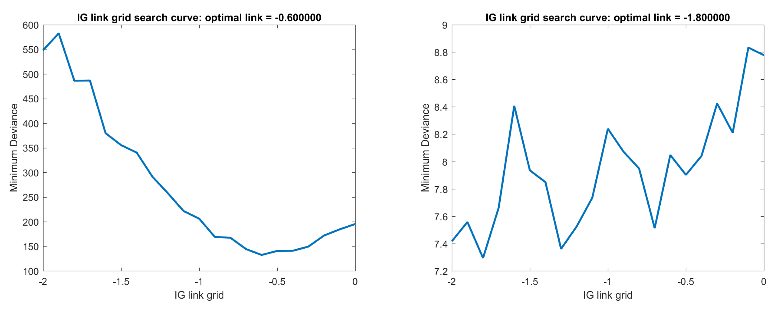
Hence, we need to find the optimal link function for the IG GLM LASSO regression. We use a grid search to attain the minimum deviance in the range of ($-2,0$) to find the optimal power link function. Deviance is the log-likelihood difference between a saturated model and a selected submodel. For given fixed design matrix, the log-likelihood of the saturated model is fixed. Hence, minimizing deviance is equivalent to finding the maximum log-likelihood of the selected model.

The grid search path curve on one set of simulated data set with link function =$-0.5$ is illustrated in Figure 1. We also simulated with three different link functions in the data generation process as $[-0.5,-1.0,-1.5]$ and simulated 10 times for each link function. We used a grid search to recover the true link function as illustrated in

Table 4. Optimal IG link grid search on simulated data.

True Link	Optimal Link Based on Minimum Deviance for Simulated Data
	Mean	1	2	3	4	5	6	7	8	9	10
−0.5	−0.48	−0.7	−0.3	−0.6	−0.6	−0.6	−0.4	−0.2	−0.2	−0.5	−0.7
−1.0	−1.14	−1.6	−0.8	−0.5	−2.0	−0.1	−1.0	−1.4	−1.2	−1.4	−1.4
−1.5	−1.31	−1.5	−0.9	−1.8	−0.5	−1.2	−1.6	−1.1	−1.2	−1.8	−1.5

When true link When the true link function is far away from the canonical link, such as $-0.5$, using grid search of the minimum deviance works better. This can be seen from a smaller search variance of repeated simulations on the $-0.5$ true link, compared with the variances of the true link $-1$ and $-1.5$.

. We find that the mean optimal link functions from the grid search are $[-0.48,-1.14,-1.31]$, which are close to the true link function. However, the variances are larger for the true link functions with powers $-1$ and $-1.5$, which may be because they are closer to the canonical $-2$. The grid search result from the simulated data shows that using grid search on minimum deviance can help us recover the true link function, especially when the true link function is far from the canonical link.

3.2.3. Estimation Evaluation Standards

We split the simulated data set into a training set and a test set with a 90%–10% proportion. We compared the fitting performance via four regular assessment indices: firstly, we computed the precision and recall ratio on non-zero coefficients fitted from the training set, as well as the precision and recall ratio of significant coefficients4 Secondly, we calculate MAE, RMSE, and deviance on the test set. We repeat the simulation 10 times and calculate the average performance.

(a)

Precision and recall for non-zero coefficients identified: to identify and count the number of non-zero coefficients, we compute the proportion of the selected covariates, which are correct as precision and the proportion of true covariates correctly selected as recall. First, we count the number of true positive (TP), false positive (FP), and false negative (FN), then we compute $Precision=\frac{TP}{TP+FP}$ and $Recall=\frac{TP}{TP+FN}$;

(b)

Precision and recall for significant coefficients identified: similar to chapter 18 of Hastie et al. (2001), we define and identify regression coefficients as significant if $|\frac{\widehat{{\beta }_j}}{\widehat{s{e}_j}}|>2$, which is equivalent to being outside of a 95% confidence interval. Then we compute precision and recall the same as (a). However, here we cannot get standard errors of coefficient estimates from a GLM LASSO computing package. Hence, we calculate $\widehat{{\beta }_j}$ and $\widehat{s{e}_j}$ from fitting a GLM, which only fits the response on the selected non-zero covariates. This is also called the relaxed LASSO. Hence, here, significance is defined as statistically below 5% level in a GLM regression, which arises from the relaxed LASSO.

(c)

MAE and RMSE: mean absolute error on test set, computed as $mean\left(abs(\widehat{y}-y)\right)$; root mean square error on test set, computed as $\sqrt{mean{(\widehat{y}-y)}^2}$. However these two evaluations are not stable; some extreme values may have large impacts on the result.

(d)

Deviance: this is the log-likelihood difference between saturated model and current model, calculated as $Deviance=2[{\ell }_{saturated}-{\ell }_{current}]$; deviance can be obtained directly from the output of the GLM LASSO fitting packages.

3.3. Simulations under Various Scenarios and Corresponding Estimation Evaluations

We investigate the model performance under different fitting scenarios. There are three items we can change. We only compare the performance when each of the four items is changed from the base case scenario, instead of when their combinations are changed. The items we will change are as follows:

(a)

collinearity level, i.e., the correlation coefficient between covariates. The LASSO model actually cannot deal with collinearity very well; we expect bad fitting results from highly correlated covariates;

(b)

sparsity level, i.e., sample size and covariate numbers n and p; LASSO models are designed to deal with sparsity; we expect no big difference when we vary the sparsity level;

(c)

SNR, signal to noise ratio will affect the capacity of the model to identify correct covariates. We expect the fitting result to be worse, when we decrease the SNR level.

3.3.1. Base Case Scenario and Parameter Optimization

We define base case scenario as: (i) no collinearity; (ii) sample size $n=128$ and covariate dimension $p=420$, which are the same size as the design matrix of the real world macroeconomic data in Section 4; (iii) covariates generated from Gaussian distribution $normal(0,1)$ and deviates dispersion parameter $\sigma$ calculated from SNR=10, respectively for Gaussian and IG deviates; (iv) set the coefficients of all 4 non-zero covariates equal to 1.

We first fit the base case scenario with univariate Box–Cox transformation ${\lambda }_{BC}$ and canonical link $g\left(\mu \right)={\mu }^{-2}$ as in Figure 2 and Figure 3. We call these the simple models; then we fit the base case scenario with iterative three-phase optimal ${\lambda }_{BC}$ and optimal link function from grid search on minimum deviance as in Figure 4. We call these the optimized models.

From the trace plots in Figure 2, we can easily see that there are four covariates noticeably different from the other covariates. However, the subset selected by either the minimum deviance fitting or the 1SE deviance fitting includes a much larger number of covariates than 4. Comparing the cross-validated deviance curve plots, we find that BC-ig model gives us smallest SE relative to the other models. In LASSO models, the larger the penalization parameter, the less covariates selected. Hence, specifically for our simulated model with only a few true covariates, the BC-ig model should perform worst due to its smallest SE. From the cross-validation plots, we cannot find significant difference between the simple models and the optimized models.

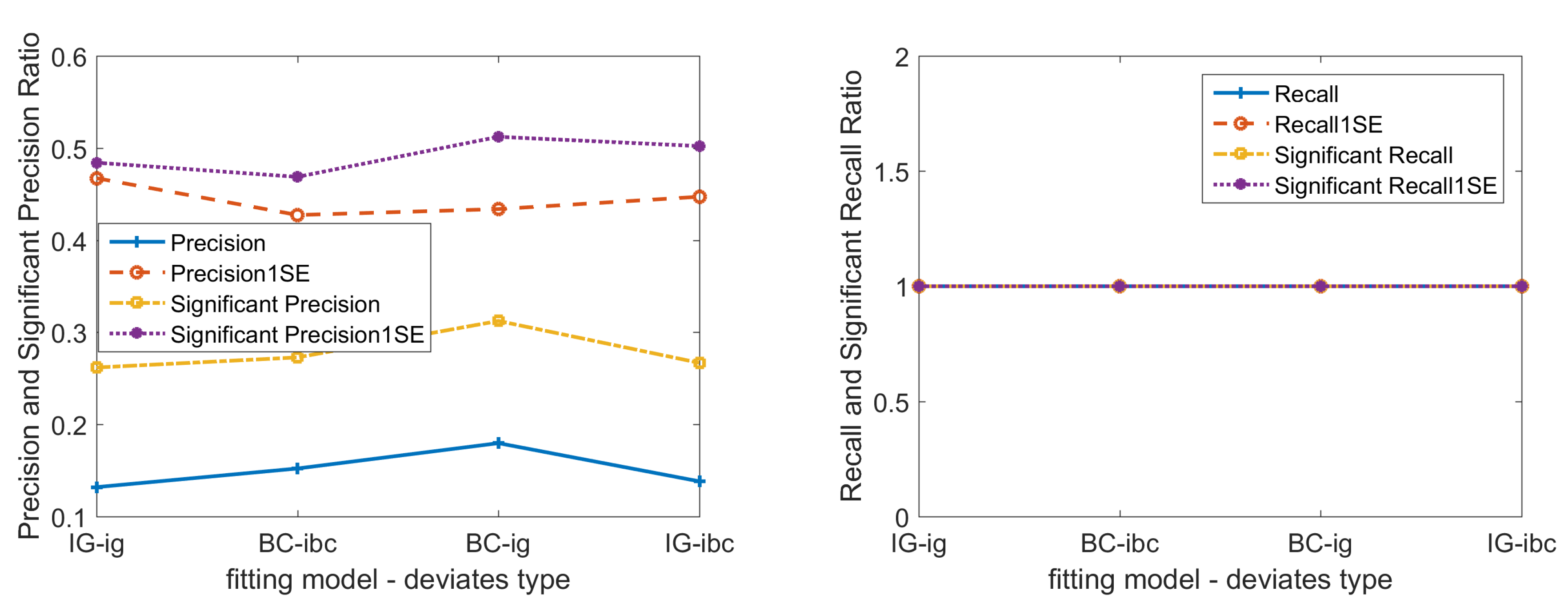
Comparing the error evaluation performance of simple models and optimized models in Figure 3 and Figure 4, we find that optimized models outperform simple models in all error evaluation criteria, i.e., MAE, RMSE, and deviance of simple model fittings are much larger than that of optimized models. To evaluate the performance in finding true non-zero covariates we use the recall ratio and the precision ratio. Simple fittings and optimized fittings both perform very well at recall ratio = 1, and roughly the same at significant precision ratio around 0.5. Here we need to mention that: when we use significant covariates to calculate the precision ratio, we can significantly improve the ratio from below 0.2 to around 0.5. We find that the optimized model outperforms the simple model in error evaluation criteria. Hence, we will use optimized models in the rest of the paper.

We also find that the optimal power of the link function for the IG GLM LASSO model is close to the optimal Box–Cox transformation parameter ${\lambda }_{BC}$, i.e., around true parameter $-0.5$, which means the latter can provide us with a good clue for a better link function.

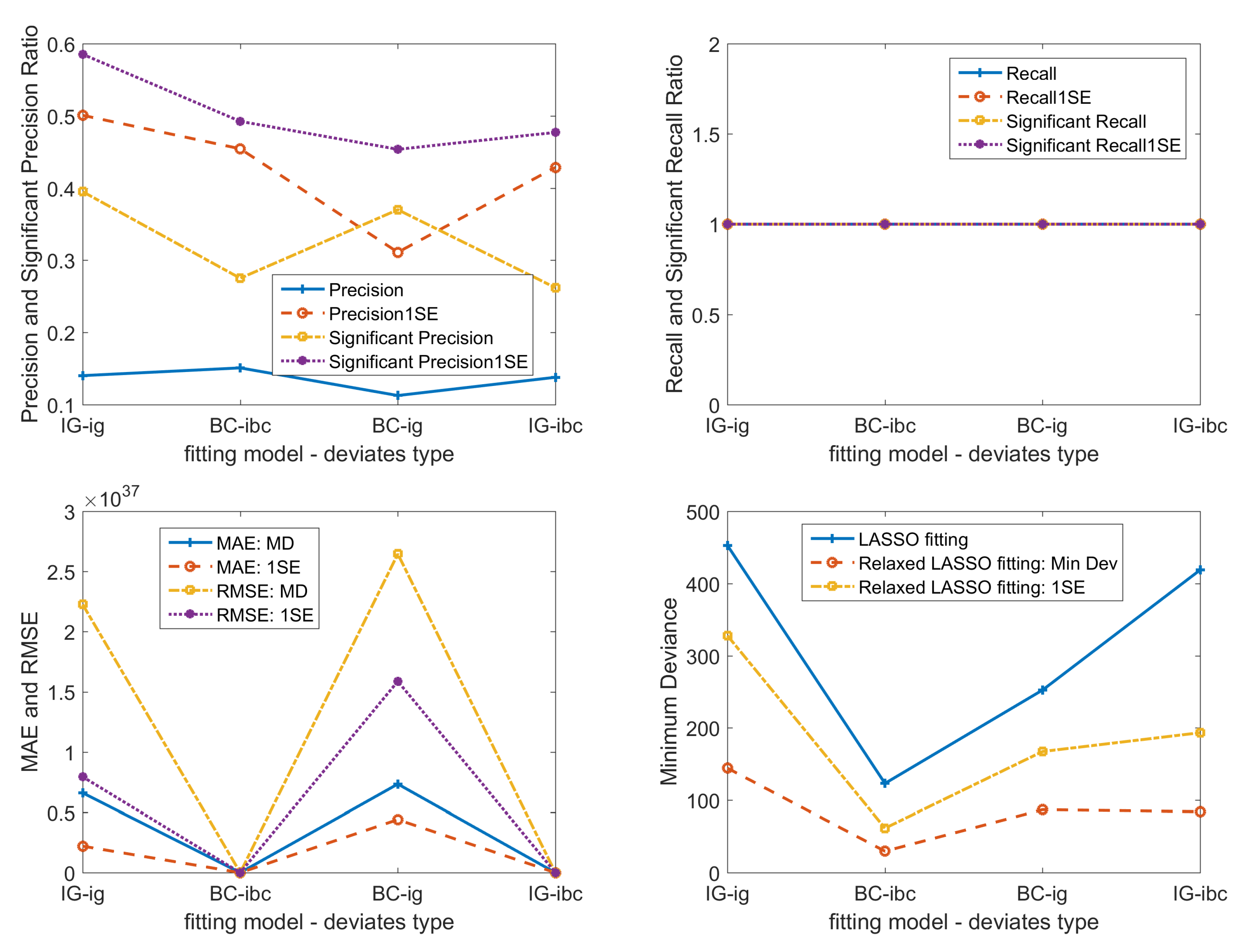
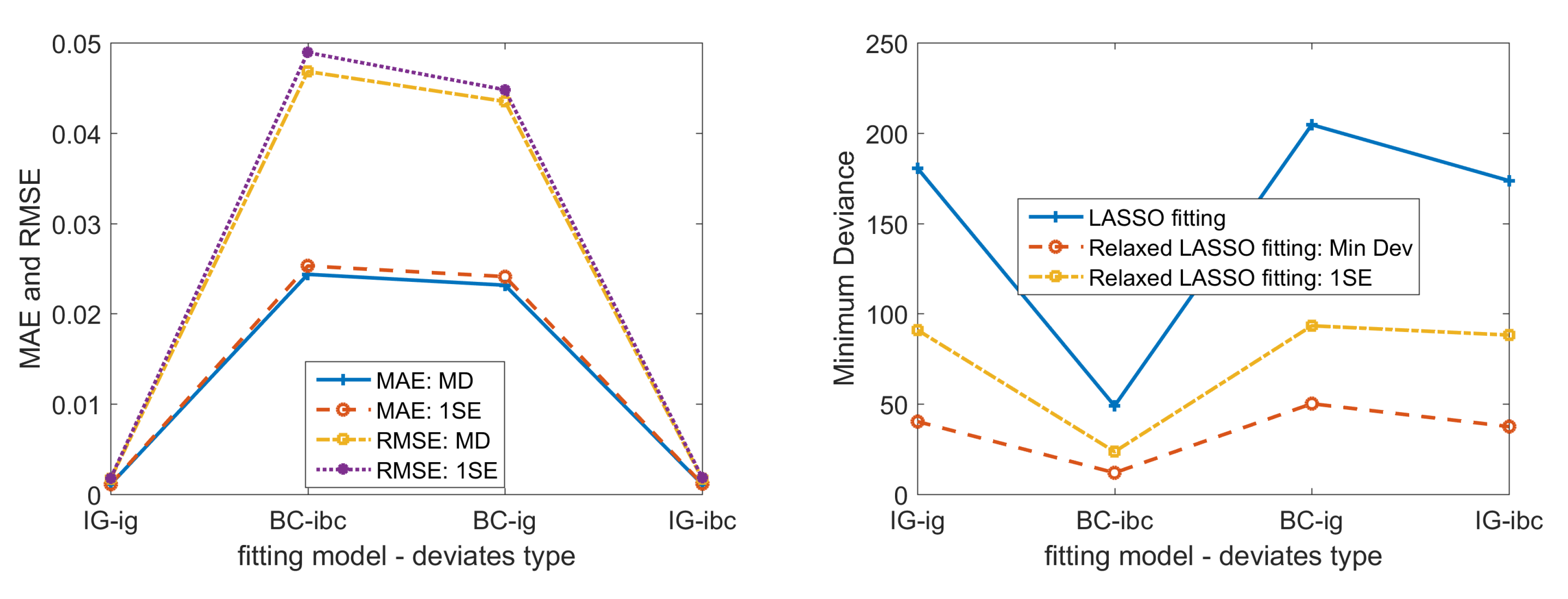
With parameter optimized fitting models under base case scenario, as illustrated in Figure 4, we find that:

(a)

Compared with the initial LASSO selected covariate subset, significant covariates of relaxed LASSO GLM fitting can improve the precision ratio from below 0.2 to round 0.3, at the same time keeping the recall ratio at 1.0. Even with 1SE fittings, significant precision ratio can still increase a little bit. This further validates that we can use significant covariates to get a more interpretable covariate subset than the initially LASSO selected subset.

(b)

Compared with the BC Gaussian LASSO model, the IG GLM LASSO model gives us smaller fitting MAE and RMSE, as well as a little bit higher precision ratio.

(c)

Fitting results on $Y_{ibc}$ deviates has smaller deviance, compared with those on $Y_{ig}$ deviates.

(d)

For precision ratio, we find no significant difference between IG models and BC models.

3.3.2. Collinearity Level Influence

Ridge regression is devised to deal with the collinearity problem. LASSO regression can also process covariates with collinearity embedded and find the most significant covariate subset. From simulation, we find that our IG GLM LASSO model and Box–Cox transformed Gaussian model can both recover the true covariates when collinearity is only introduced between non-zero and zero covariates; however, if there is collinearity among non-zero covariates, the fitting result will dramatically worsen as the correlation level increases.

Firstly, we introduce collinearity between non-zero covariates and zero covariates. Both BC model and IG model can treat collinearity between non-zero and zero covariates very well. We find no big differences in all the fitting performance evaluation criteria.

Secondly, we introduce collinearity among non-zero covariates, with low correlation in range $[0.1, 0.4]$ and high correlation $[0.6, 0.9]$, respectively. We find that LASSO method cannot recover all of the true covariates for ig deviates, with a recall ratio below 1. However, the precision ratio is roughly the same and even increases a bit as the correlation level increases. At the same time, the fitting errors also increase significantly for the ig deviates.

From the simulation result, we find that only the BC-ig combination gives a poor fitting result, especially when the correlation increases. The fitting performances of most of the combinations, i.e., IG-ig, BC-ibc and IG-ibc, are roughly the same as that of the scenarios without collinearity introduced. Hence, we conclude that the LASSO model can deal with collinearity very well, especially when we fit the response with the ’correct’ GLM LASSO model. The above simulation analyses validate that we can use LASSO model to fit a data set with covariates composed of correlated economic and financial time series data.

3.3.3. Sparsity Level Influence

We also want to check how the sample size, as it relates to to the covariate dimensionality, impacts the model fitting result; we refer to this as the sparsity level. Fixed at 4 non-zero covariates, the same as base case scenario, we change the sample size n and covariates dimension p to change the sparsity level.

Firstly, we change the sample size n from 128 to 1280 and keep the covariate dimension at 420. Secondly, keeping the sample size at 128, we increase the covariate dimension from 420 to 4200. We find that whether $n\ge p$ or $n<<p$, the relative performance of the four combinations stays the same. As we increase sample size n, precision ratio increases toward 1; as we increase covariate dimensionality p, recall ratio decreases below 1.

3.3.4. SNR Level Influence

In this part, we vary the SNR ratio, as we defined in Section 3.1, to check the model fitting performance. High SNR ratios make it easier to capture the true covariates, vice versa for low SNR.

Comparing the fitting performance when SNR equals to 100 and when SNR equals to 2, we find that both models perform better when SNR increases and worse when SNR decreases. However, the IG model performs better than the BC model, especially in the precision and recall ratio, irrespective of whether SNR increases or decreases. Hence, the IG model is more robust to SNR changes, in comparison with the BC model.

3.4. Some Concluding Remarks on Our Simulation

Applying the Box–Cox grid search on a LASSO model is hard, because each penalization parameter ${\lambda }_{lasso}$ will result in a different subset of covariates selected. Different subsets make their log-likelihood non-comparable to each other and left us with a very uneven and rough grid search path curve. In this paper, we used an iterative three-phase optimization method to find an optimal ${\lambda }_{BC}$. It is worth noting that when using the IG GLM LASSO model, we should not rely on the canonical link, even if it has better statistical properties. Sometimes the true link function is far from the canonical link; hence, we should try to optimize the link function. We used a grid search on minimum deviance to find the optimal link function and the simulation results show that the optimal IG link performs better on all our evaluation criteria. From the simulations we also find that the optimal Box–Cox transformation parameter provides a good estimate for the optimal IG link function as they are very close to one another. As collinearity does not have a big impact on the fitting performance in a simulated data set, we only did a preliminary filtering when we collected the real world data and we did not perform further collinearity checks in this paper. We also note that the SNR ratio will influence the performance of the fitting and we find the IG model to be more robust. However, the Box–Cox model is easier to use since it is Gaussian distributed after transformation and we will use both models for the real world data. Finally, sparsity does not have a huge impact on the fitting performance and the sample size of our real world data are large enough for us to produce a reliable fitting result.

4. Empirical Study: U.S. Stock Market Volatility Forecast

The stock market as a whole has its own boom and bust cycles, which are the collected movements of all the stocks in the market; undoubtedly, stock market volatility indices are impacted by the macroeconomic environment, firm profits, market evaluation level, and people’s herding behavior.

In this section, we apply four LASSO models as in the simulation section to study stock market volatility. They are IG GLM LASSO model with optimized link and canonical link, respectively; Box–Cox transformed Gaussian LASSO model with three-phase iteratively searched Box–Cox ${\lambda }_{BC3P}$ and univariate Box–Cox ${\lambda }_{BC}$, respectively. Beyond fitting and forecasting stock market volatility with the accessible data, our top priority is to identify some leading indicators to help us forecast quarterly U.S. stock market volatility. To make the study period as long as possible, we use macroeconomic data and industry level financial ratio quarterly data; some alternative data sources such as google search data have a short record, so we have not included them in our study.

Using LASSO models as a dimension reduction method, we find some ‘robust’ covariates. We define it as a ‘robust’ covariate if the covariate is statistically significant in more than one of the four LASSO models. We can track these ’robust’ covariates as an early warning signal to help us forecast when the stock market volatility may face a change of trend in near quarters.

4.1. Dataset

We collected quarterly macroeconomic data, financial market data, and industry level financial ratio data and we separated them into two data sets.5 There are four stock market volatility indices, i.e., VXO implied SP100 index volatility, SP500 index realized volatility, Wilshire 5000 index realized volatility, and NASDAQ index realized volatility. Per our distribution check in the previous section (Section 2.1), we find that VXO implied SP100 index conforms better to the IG distribution, so we will use VXO index as our response variable. There are also 98 other macroeconomic and financial market indicators across a wide range of economic aspects in the list, such as:

(1)

Interest rates (e.g., federal fund target rate, 30-year mortgage rate) and bond yield spreads (e.g., 10-year minus 2-year treasury yields spread, 10-year Aaa corporate bond minus treasury yield spread);

(2)

Credit expansion and money supply (e.g., commercial and industrial loans, M1 and M2 supply);

(3)

Inflation rate (e.g., consumer price index for all urban consumers: food, personal consumption expenditures excluding food and energy, WTI oil price);

(4)

Industrial production and sales (e.g., industrial production index, capacity utilization, GDP growth rate, real manufacturing and trade industries sales);

(5)

Employment (e.g., non-farmer payroll, unemployment ratio, average hourly earnings of production and non-supervisory employees, civilian labor force);

(6)

Investment and housing market (e.g., private nonresidential fixed investment, new privately-owned housing units under construction, house price index)

(7)

Savings rate and consumption (e.g., personal saving rate, university of Michigan: consumer sentiment);

(8)

Debt and deficit level (e.g., fiscal deficit, balance of payments, household debt);

(9)

Others (e.g., SP500 PE ratio, total vehicle miles traveled, trade weighted U.S. dollar exchange rate index).

There are 65 industry level financial ratios for 10 industry groups of the SP500 index. The ten industry groups are: durable goods, non-durable goods, energy, HITEC, Health, Manufacturing, SHOPS, Telecommunication, Utilities, and others. The 65 industry level financial ratios include most of the popular financial evaluation ratios, for example: return as a percentage of the price, price to earning growth (PEG) ratio, book to market ratio, asset turnover, etc.

We used the augmented Dickey–Fuller (ADF) test to test the stationarity of our data sets. Four volatility response variables passed the test, which indicates they are stationary time series and do not have a unit root. However, most of the macroeconomic time series are not stationary. Hence, we took first order differences on the log transformed series and then used the ADF test to perform a unit root test. For the indicators that did not pass the ADF test, we took second differences, and found that all passed the test. Hence, all the covariates we include in the design matrix are also stationary time series.

After differencing: we had a quarterly macroeconomic data set with 98 indicators and 133 observations ranging from 1986Q3 to 2019Q3, and quarterly industry level financial ratio data set with 650 indicators and 130 observations, ranging from 1986Q3 to 2018Q4.

Inspired by Drikvandi (2019), we used the top 30 principle components6 of the financial ratio data set as a substitute for the raw financial ratio data set, since they are highly correlated. We used the singular value decomposition (SVD) method to obtain the principle components. Firstly, we decomposed the whole Financial ratio data set $X_{130\ast 650}$ into three matrices $X=UD{V}^T$, where $U_{130\ast 130}=(u_1,\cdots ,u_{130})$ ($u_i$ is a column vector), $V_{650\ast 650}^T=(v_1,\cdots ,v_{650})$ ($v_i$ is a column vector), and $D_{130\ast 650}=(d_1,\cdots ,d_{650})$ ($d_1$ to $d_{130}$ are vectors with only 1 non-zero element and $d_{131}$ to $d_{650}$ are zero vectors). Secondly, we selected the top k principle components $Y_{130\ast k}=U(:,1:k)\ast D(1:k,1:k)\ast V{(1:k,1:k)}^T$. This matrix $Y_{130\ast k}$ provides a reconstruction of the original data from the first k PCs. Or we simply use the first k PCs, $Y_{130\ast k}=U(:,1:k)\ast D(1:k,1:k)$. There are no big differences between these two kinds of reconstructed PCs and they give us roughly the same covariate subsets.

To find the leading indicators, we used data one to four quarters ahead to form a design matrix to fit our model. Hence, we had three design matrices: $macr{o}_{129\ast 392}$ ranging from 1987Q3 to 2019Q3, ${(macro+FinR)}_{126\ast 2992}$ ranging from 1987Q3 to 2018Q4, ${(macro+PC30)}_{126\ast 512}$ ranging from 1987Q3 to 2018Q4. We divided the data set into a training set and a testing set as 90%:10% of the total observations in time order. We evaluated the fitting performance on three error criteria, as well as explored graphically both in-sample fitting and out-of-sample forecasting plots. We also compared our multivariate LASSO fitting results with univariate time series fittings, i.e., NAIVE model and ARMA(1,0) models.

4.2. Fitting Results

We fit VXO implied SP100 volatility index as the response variable with four models, the same as in Section 2, on three data sets, i.e., macroeconomic data set, macroeconomic + financial ratio data set, and macroeconomic + PC30 data set. To estimate the response, the relaxed LASSO gives us the best fitting results. Hence, all fitting figures and tables use the results from the relaxed LASSO.

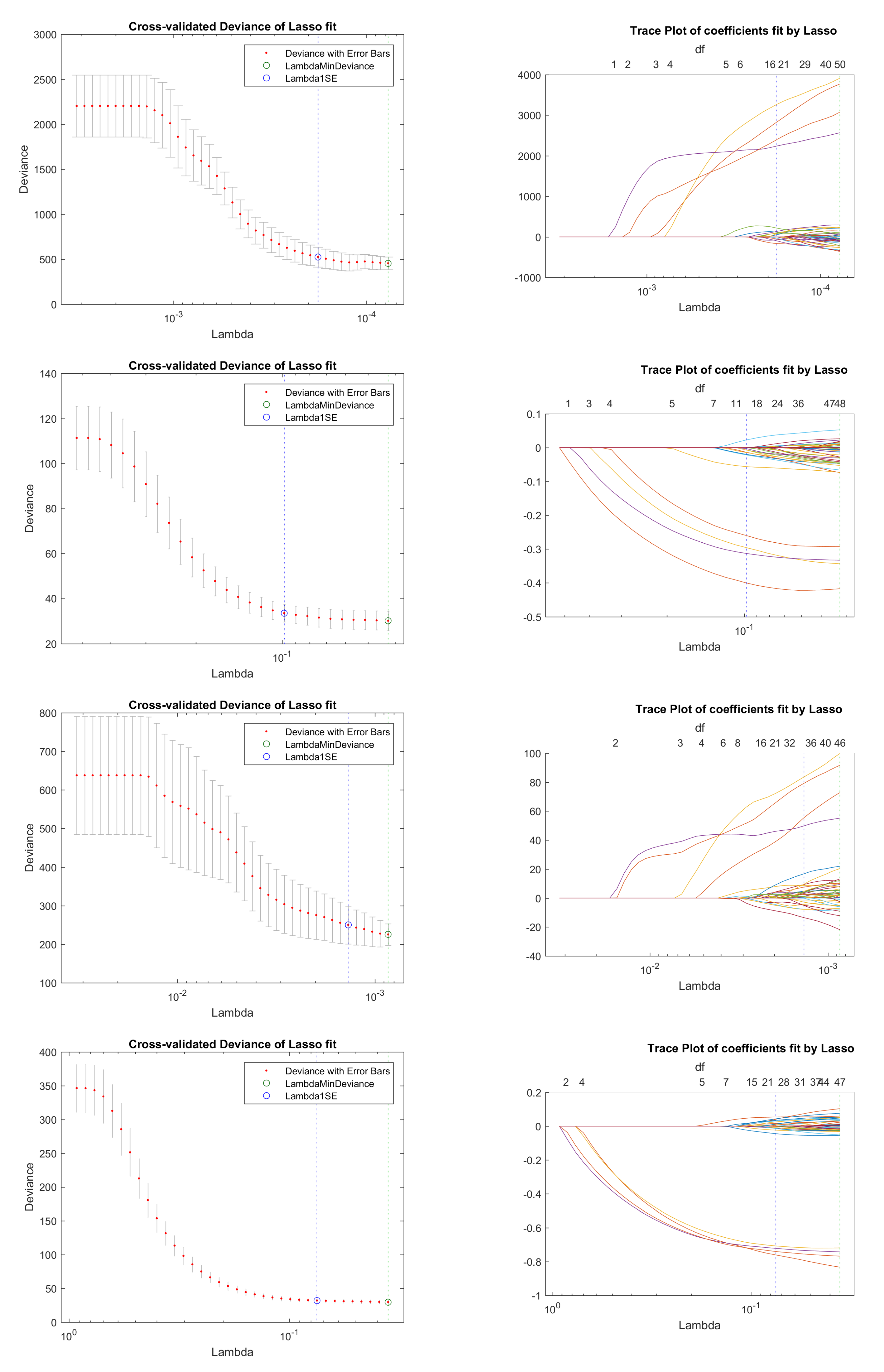
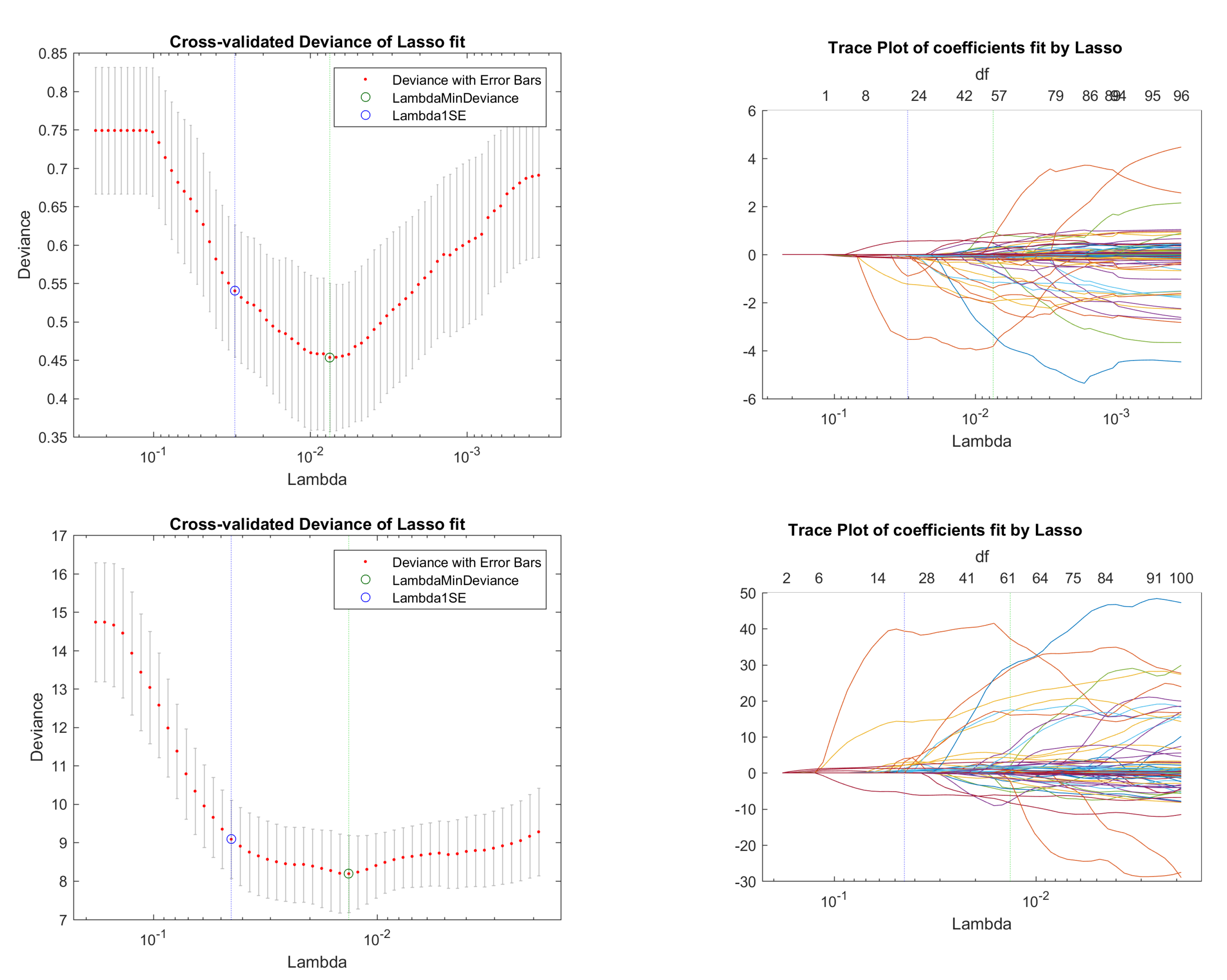
Firstly, we plotted the cross-validation and trace plots to illustrate the shrinkage trace in Figure 5. We can easily see that the shrinkage method can efficiently choose a small subset. Secondly, we compared the fitting results of each model and the subsets selected. We wanted to compare which model was the best one among four models and to identify some common covariates, which could help us to forecast the stock market volatility.

We compared the out-of-sample forecasting error evaluation criteria MAE and RMSE, and in-sample 5-fold cross-validated Deviance, in summary

Table 5. Fitting error evaluation summary: VXO.

Covariates	Fitting Model	MAE (%)	RMSE (%)	Deviance	Significant Covs
Univariate7	Naive	3.17 (3.48)	4.53 (6.00)	n.a.	n.a.
	ARMA(1,0)	3.06 (4.32)	4.74 (6.87)	n.a.	n.a.
Macro	IG(−0.10)	4.70	5.18	0.0389	27
	BC(0)	4.18	4.75	0.1683	35
	IG(−2)	4.70	5.61	0.2248	10
	BC(−0.51)	4.62	5.48	0.0818	19
Macro + FinR	IG(−0.20)	4.78	5.54	0.1896	10
	BC(0)	5.43	5.89	2.7546	13
	IG(−2)	5.46	6.19	0.4386	5
	BC(−0.48)	4.75	5.31	0.1664	14
Macro + PC30	IG(0)	3.39	4.47	0.0201	36
	BC(0)	3.84	5.00	0.3291	31
	IG(−2)	4.43	5.17	0.2224	11
	BC(−0.48)	3.58	4.61	0.0845	36

1. We fit the VXO volatility index on three data sets: macroeconomic data set, macroeconomic + financial ratio data set, macroeconomic + top 30 principle components data set. 2. We fit with four models for each data set: optimized link function IG GLM LASSO model, three-phase iteratively searched Box–Cox ${\lambda }_{BC3P}$ transformed Gaussian LASSO model, canonical link IG GLM LASSO model, and response only univariate Box–Cox ${\lambda }_{BC}$ transformed Gaussian LASSO model. 3. The error evaluation criteria are based on relaxed LASSO fitting results.

. We found that some of them show somewhat smaller errors, such as the fit of Macro + PC30 data set with the optimal IG link model. However, there is no big difference in general. We also found that, as more significant covariates are used, smaller fitting errors result.

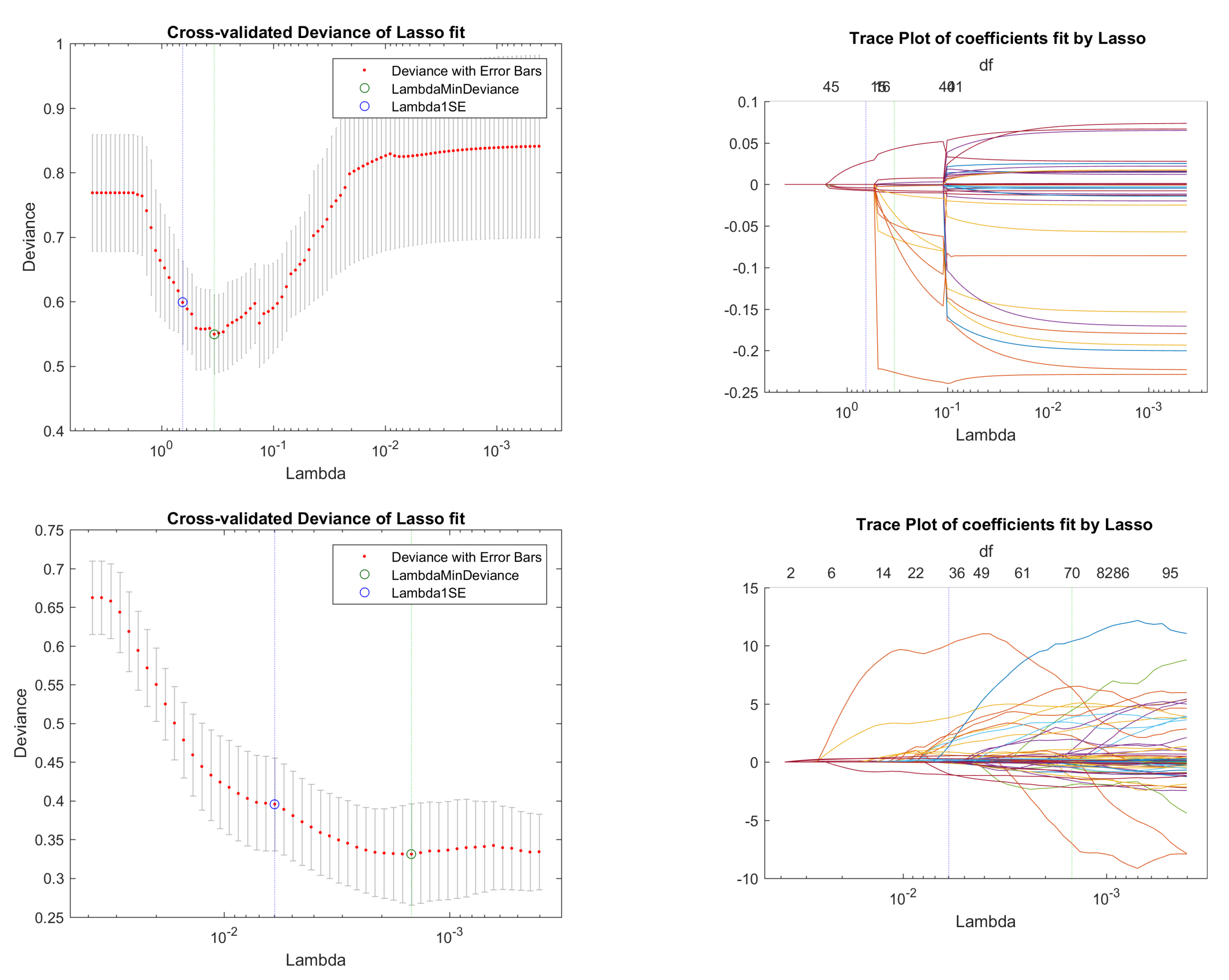
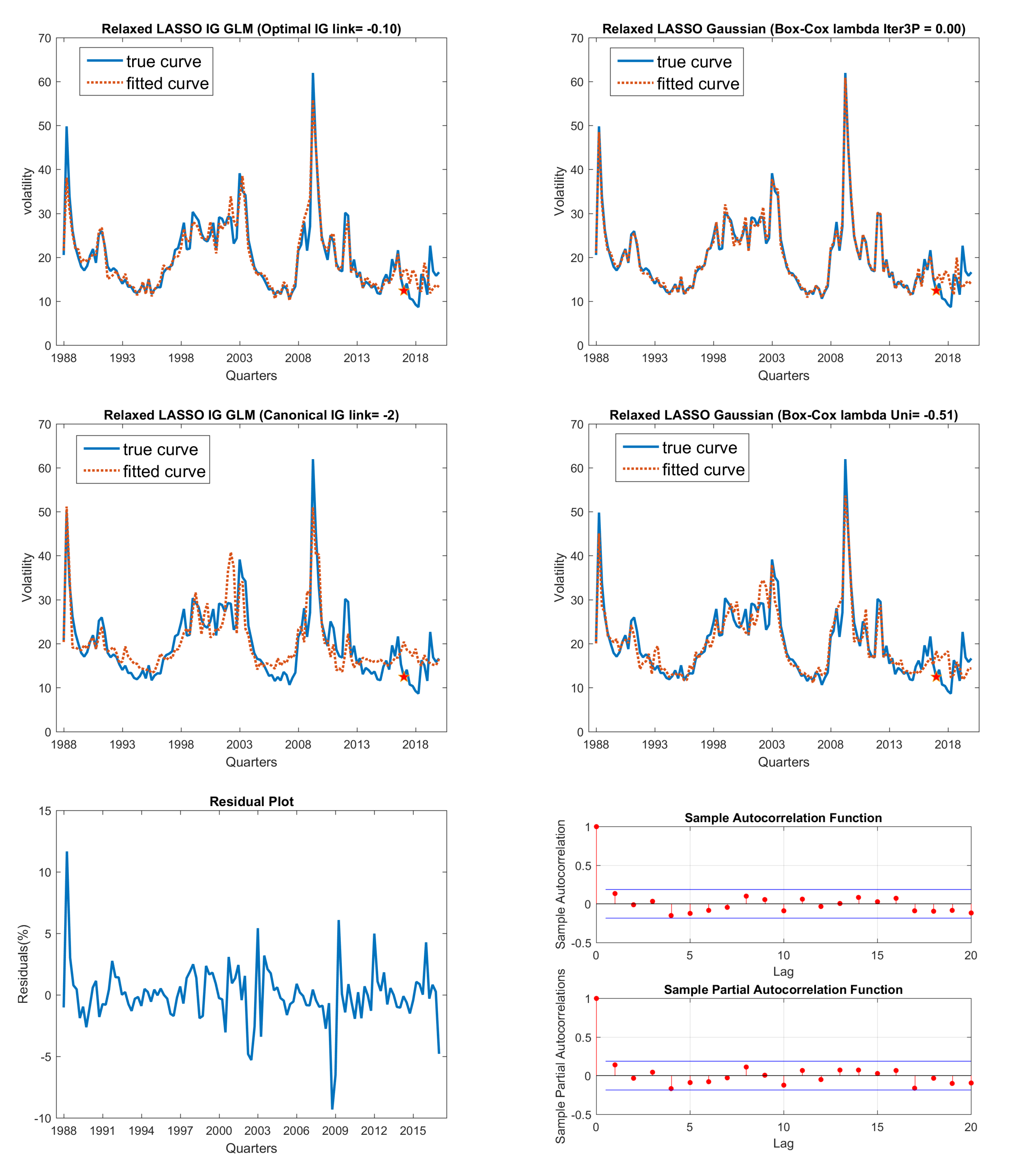
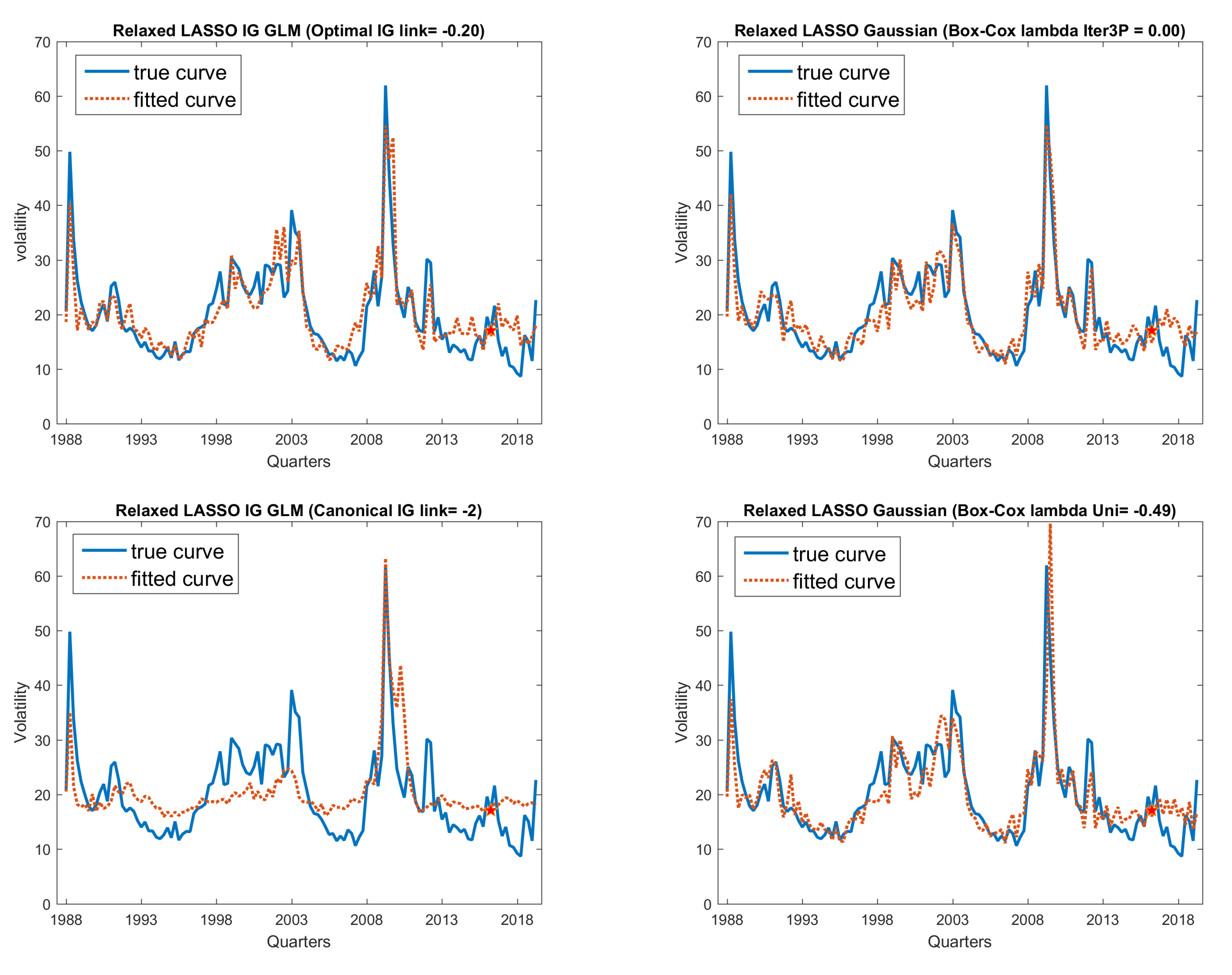
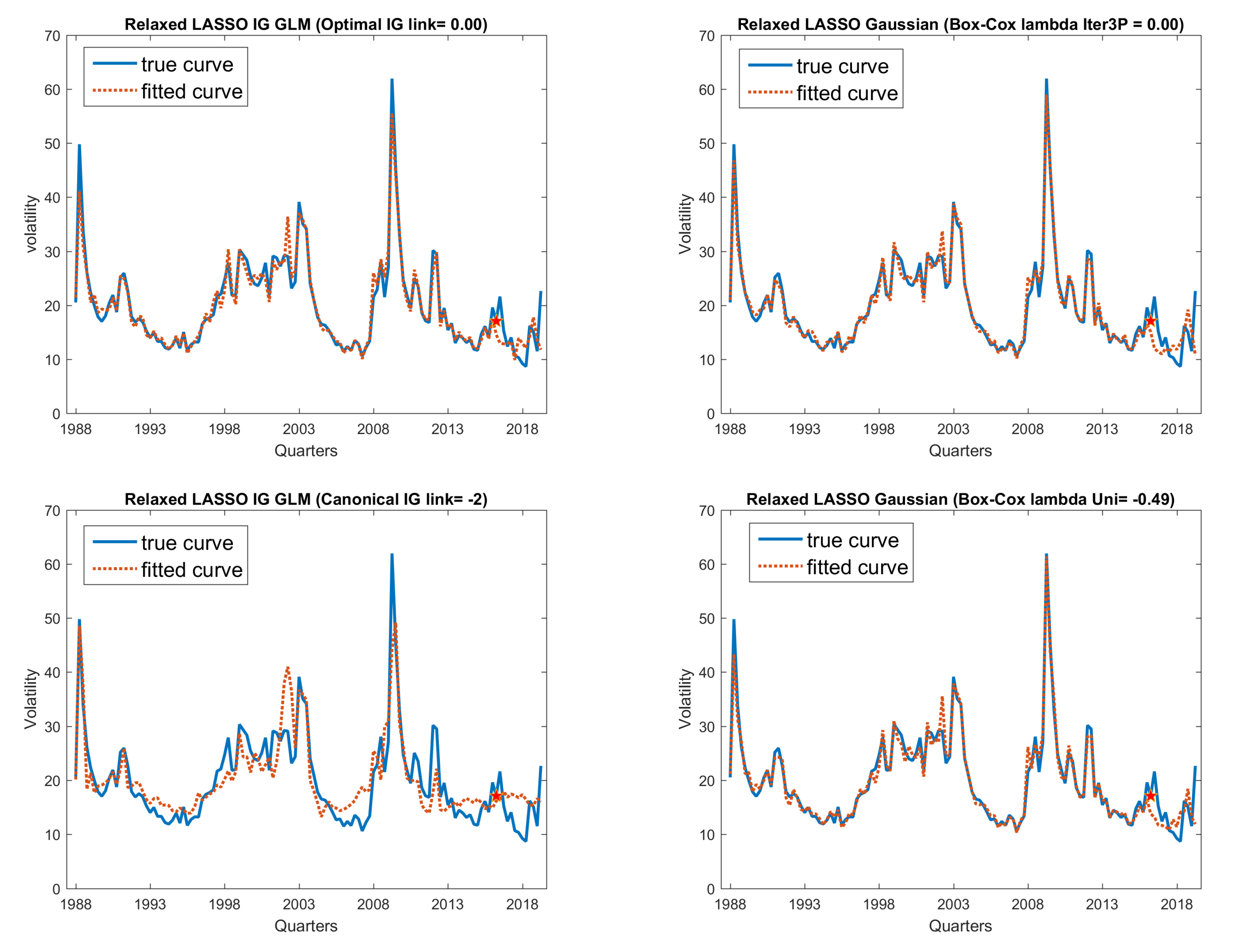
We plotted four sets of relaxed LASSO fitted curves and true curve comparison Figures. They are Figure 6 on the Macroeconomic data set, Figure 7 on the significant covariates of the macroeconomic data set, Figure 8 on macroeconomic + financial ratio data set, and Figure 9 on macroeconomic + top 30 PCs data set. From these figures, we can easily see that most of the in-sample fitting results are very good; however, some of the out-of-sample forecasts are not good. Intuitively, the good fitting curve captures the turning points of the trend better than the bad ones. Among these Figures, we find that two combinations have better out-of-sample fitting results: the first of these, in Figure 7, fits on significant covariates of the macroeconomic data set, are the two Box–Cox transformed Gaussian LASSO models; the second of these, in Figure 9 with macroeconomic + PC30 data set, are all four models except the canonical link IG GLM LASSO model. This implies that by extracting principle components from the financial ratio data set, we can improve the out-of-sample forecasting.

The reason that the out-of-sample forecasting is not as good as the in-sample fitting results is that we did not collect every related factor in our covariates data set. For example, some abruptly occurring events, e.g., conflicts between countries, natural hazards, and pandemics, also have a huge impact on the stock market volatility. This kind of abrupt occurring event rarely happens, but once it happens, the stock market will show chaotic fluctuations. Our study in this paper only captures a partial picture of the true evolving mechanism of the stock market. To be more specific, the impacts due to the fundamental economic cyclical change.

Looking at our LASSO fitting results, we find that several dozens of covariates are selected in each LASSO non-zero subset; the number of the selected covariates is much greater than that of the significant ones illustrated in summary Table 5. Moreover, covariate subsets will also change if we fit it the second time due to cross validation re-grouping. Hence, we only analyzed and interpreted the significant covariates and we further tagged the covariate as ‘robust’, if the covariate was selected as significant in more than one data set.

In this paper, we mainly focused on identifying the ‘robust’ factors from our fundamental economic and financial data set. We believe that we can track these ‘robust’ factors to anticipate the stock market volatility change due to fundamental economic environment changes further ahead than the univariate time series models, such as the GARCH model mentioned in previous sections.

Significant covariates in the LASSO GLM fittings and the ‘robust’ ones among them are listed in

Table 6. Significant and Robust Covariates: VXO.

Fitting Data Set	Selected Significant Covariates
	Macro	Financial Ratio	PC30
Macro data	9,17,18,26,27,30,
	34,46,50,58,72,73,77,
	80,81,84,87,90,91,95
Macro + FinR data	17,58,77,91	20,41
Macro + PC30 data	5,11,17,21,26,27,34,46,
	55,57,58,62,63,72,76,		105,107,110,117,118
	81,84,87,90,91,94,95
‘Robust’ ones	17,26,27,34,58,72,77,81,84,87,90,91,95

1. Significant covariates: similar to our definition in the simulations of Section 3.2.3, when $|\frac{\widehat{{\beta }_j}}{\widehat{s{e}_j}}|>2$ in the LASSO GLM fitting, which is equivalent to being outside of a 95% confidence interval, the $j\mathrm{th}$ covariate is statistically significant; but here, we tag the covariate as a significant covariate only if it is selected by more than one of four LASSO models as statistically significant. 2. ‘Robust’ indicator: if a covariate is selected by more than one data set as a significant covariate, then we deem it as a robust one.

for the VXO volatility index.

4.3. Key Macroeconomic Indicators and Interpretation

We also used three realized volatilities as response variable to find their ‘robust’ covariates on the same data sets. We found the following common ‘robust’ indicators, which were selected by more than one volatility index fittings.

17.

AAAFFM: Moody’s seasoned Aaa corporate bond minus federal funds rate.

30.

CPILFESL: consumer price index for all urban consumers: all items less food and energy in U.S. City average, more popularly known as ‘core CPI’.

34.

PCEPILFE: personal consumption expenditures excluding food and energy, also popularly known as ‘core PCE’.

60.

UEMPMEAN: average weeks unemployed;

77.

NONREVSL: total non-revolving credit owned and securitized, outstanding. Consumer credit covers most credit extended to individuals, excluding loans secured by real estate. Non-revolving credit includes motor vehicle loans and all other loans not included in revolving credit, such as loans for mobile homes, education, boats, trailers, or vacations. These loans may be secured or unsecured.

85.

PRFI: private residential fixed investment.

90.

NCBCMDPMVCE: non-financial corporate business debt as a percentage of the market value of corporate equities. Percent, Quarterly, not seasonally adjusted.

91.

CBLBSNNCB: non-financial corporate business; corporate bonds; liability, level.

These identified common indicators are supposed to have closer correlation with the stock market volatility than other macroeconomic indicators. These indicators are more sensitive to the macroeconomic cyclical changes and they can help forecast the long-term volatility trend. Among them, the most common ones are 17 (Aaa corporate bond yield spread over Federal Funds Rate), 77 (total outstanding non-revolving credit) and 91 (non-financial corporate bonds issued).

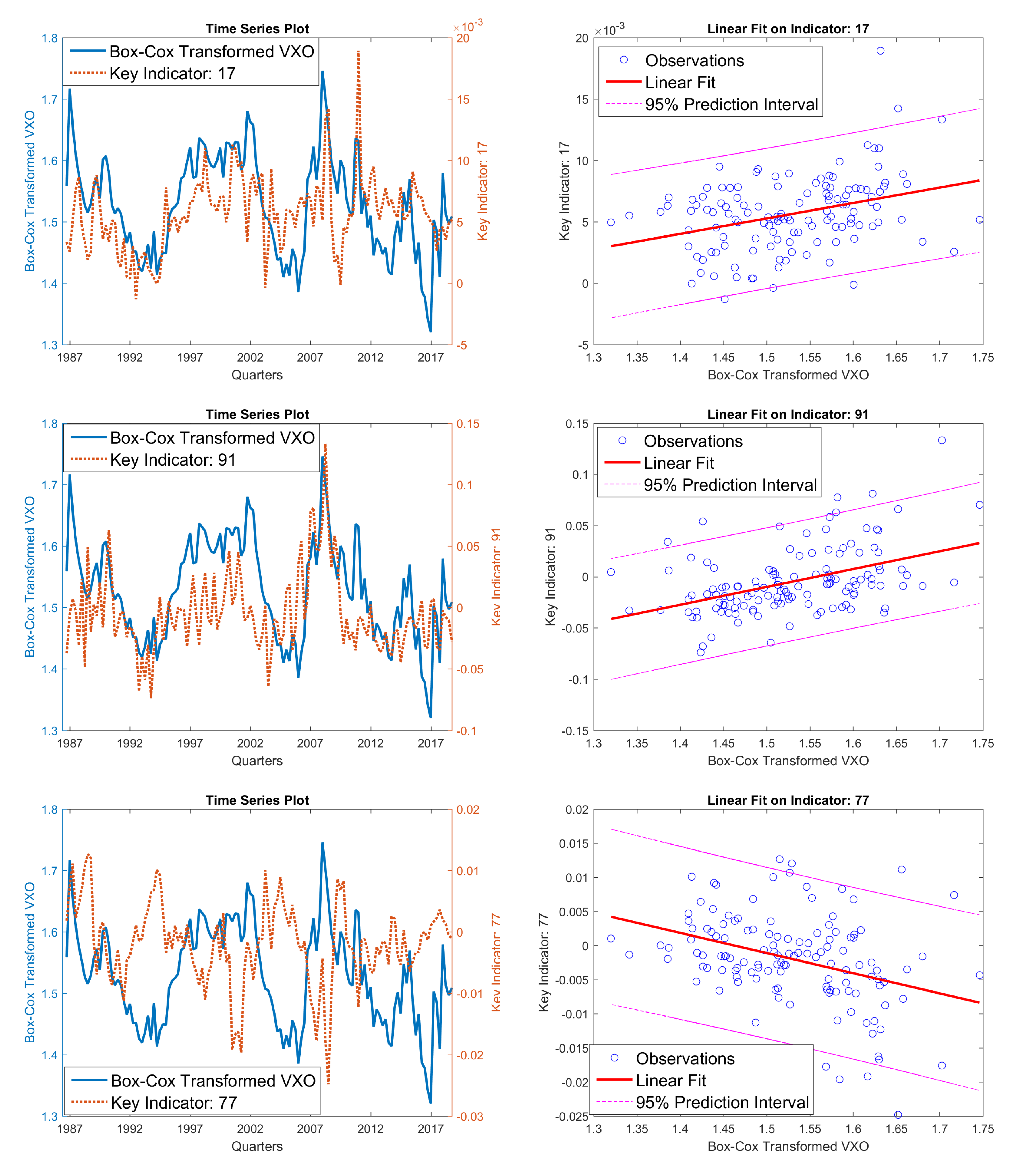
To further study the relationship between the most common ‘robust’ indicators and volatilities, we used the paired plot and the linear fitting plot to illustrate their relationship graphically. In Figure 10, we plotted both the Box–Cox transformed VXO implied volatility with the three most common significant indicators (leading 1 quarter) in one plot to provide an intuitive illustration of the relationship between stock market volatility and macro economic indicators. We also plotted a simple linear fit between the Box–Cox transformed volatility and identified indicators. From the time series plot and linear fitting plot, we can easily see the relationship between economic indicators and the VXO volatility. We find that VXO volatility will increase when indicators 17 and 91 increase, and when indicator 77 decreases. Here, we plotted Box–Cox transformed volatility $y=\frac{y^{-0.5}-1}{-0.5}$ as response variable. Hence, the linear fitting slope has the same direction as for the raw response data.

(a)

As a bond market yield spread, indicator 17 contains the credit spread between Aaa corporate bond and the U.S. 10-year treasury, and yield curve spread between U.S. 10-year treasury and federal fund rate. Yield spreads reflect the bond market sentiment changing toward the business cycle. When the fear of an incoming economic recession surges in the bond market, the usual positive slope of the bond yield curve will invert; the yield spread will tighten, even moving to a negative regime. At the same time, stock market volatility will increase quickly. There are still other more popular bond yield spread indicators, such as TED spread and 10-year–2-year treasury yield spread, included in our data set. However, LASSO fittings choose the Moody’s Seasoned Aaa Corporate Bond Minus Federal Funds Rate yield spread and deem it more efficient in forecasting stock market volatility than other yield spreads.

(b)

Indicators 77 and 91 can be all aligned into the group of credit expansion. The credit expansion demand from Consumer section, corporate section, and the government section constitute the entire economy credit expansion demand, which is one of the most important forces that shapes the business cycle. Roughly speaking, indicator 77 is the total consumer credit excluding credit card debt. It is more related to the consumer fundamental demand for debt. Hence, it can reflect the consumer sentiment about future income. Indicator 91 is the corporate bond expansion level, which is the main credit expansion channel for U.S. corporates. These two indicators represent the credit expansion demand of the consumer sector and the corporate sector, respectively, both of which are the more active sectors in the total economy than the government sector.

(c)

Positive slope of linear fitting volatility on indicator 77 implies that the volatility will increase as the consumer sector involves more debt.

(d)

Negative slope of linear fitting volatility on indicator 91 implies that the volatility will increase as the corporate sector shrinks their debt.

Among the financial ratio data, the most common selected ones are 28, 41, 52, 59. In principle components, the most common selected one is 105. The top 10 loadings (V*S’) columns of the 7$th$ Principle Components are the following columns: 3, 16, 15, 27, 34, 10, 9, 1, 2, 17, which do not overlap with the selected financial ratio indicators above.

From the summary of previous fitting results of the four volatility measures, we can see that when we add PC30 to the covariates, we get better out-of-sample forecasting as illustrated in Figure 9. However, the selected common indicators from financial ratio data and PC30 data cannot validate each other, so we can only say that adding more uncorrelated covariates improves the fitting result.

4.4. Some Concluding Remarks on the Data Analysis

Comparing the error evaluation results of the four fitting models, we find that the more significant the covariates selected, the better the error evaluation performance; this is similar to the OLS fitting; the sum square error (SSE) is smaller whenever we include more covariates. Furthermore, among the four LASSO models, the univariate searched Box–Cox $\lambda$ transformed Gaussian model fits better for most volatilities, whereas the second best is the optimal link IG model. The canonical IG link model fits worst, while the three-phase iteratively searched BC Gaussian model are roughly the same or worse than the simple BC Gaussian model. As expected the real data fitting results are not as good as that of the simulated data. Furthermore, the selected covariates will also change when we refit the data the second time, which is due to different cross validation data subsets assigned. We want to stress that, in application to the real world data study, we mainly focused on identifying some ‘robust’ indicators that could be used to track the volatility trend turning point in advance, or to foretell the quarterly trend reversal as early as possible, instead of to forecast the volatility. We did find some common ‘robust’ macroeconomic indicators, which are selected as significant covariates by most models, and these identified indicators have very good interpretation ability.

5. Conclusions

In this paper, we explored the distribution of stock market volatility data using low frequency quarterly series, which are stationary after first order differencing. We used macroeconomic and financial market data and industry level financial ratio data as covariates, and due to the high covariate dimension, which in fact is larger than the number of observations, i.e., $p>>n$, we employed the LASSO method to achieve both dimension reduction and prediction simultaneously. Since the volatility data were not Gaussian distributed, we established that they could be fitted reasonably well with the IG distribution, as well as by using the Box–Cox transformation to transform them approximately to Gaussian distribution. Hence, for non-Gaussian distributed stock market volatility data, we used the Box–Cox transformed Gaussian LASSO model and the IG GLM LASSO model to fit the stock market volatility data.

From the simulated data, we found that it is not easy to tell the difference between IG deviates and the inverse Box–Cox transformed Gaussian deviates if we do not know the distribution beforehand. Hence, in the simulation study, we fit both the Box–Cox transformed Gaussian LASSO model and the IG GLM LASSO model to IG deviates and inverse Box–Cox transformed Gaussian deviates, respectively. In this way, we had four combinations, i.e., IG-ig, BC-ibc, IG-ibc, and BC-ig. We used a three-phase iterative grid search method to find the optimal Box–Cox transformation parameter ${\lambda }_{BC}$ based on maximum log-likelihood and we also used a grid search to find an optimal IG link function based on minimum deviance.

We fitted real world stock volatilities on macroeconomic and financial market data, as well as industry level financial ratio data. We compared the out-of-sample error evaluation performance and explored graphically via paired plots of fitted curves and true curves. There are some potential future directions for work that can extend our approach and may help us forecast the stock market volatility trend better. These include extending the data set to include more covariates and trying other LASSO models, such as group lasso, adaptive lasso, and the VAR-LASSO among others. Finally, after identifying these ‘robust’ covariates, we can use generalized additive model (GAM) instead of just linear combination of predictors to fit the response, and we can attempt to combine our pure multivariate covariate subset selection LASSO method with GARCH models, which may be more appropriate for time series data.

References

- Baillie, Richard T., Tim Bollerslev, and Hans Ole Mikkelsen. 1996. Fractionally integrated generalized autoregressive conditional heteroskedasticity. Journal of Econometrics 74: 3–30. [Google Scholar] [CrossRef]
- Bollerslev, Tim. 1986. Generalized autoregressive conditional heteroskedasticity. Journal of Econometrics 31: 307–27. [Google Scholar] [CrossRef] [Green Version]
- Box, George E. P., and David R. Cox. 1964. An analysis of transformations. Journal of the Royal Statistical Society: Series B (Methodological) 26: 211–43. [Google Scholar] [CrossRef]
- Clark, Peter K. 1973. A subordinated stochastic process model with finite variance for speculative prices. Econometrica 41: 135–55. [Google Scholar] [CrossRef]
- Desmond, Anthony F., and Zhenlin Yang. 2011. Score tests for inverse Gaussian mixtures. Applied Stochastic Models in Business and Industry 27: 633–48. [Google Scholar] [CrossRef]
- Drikvandi, Reza. 2019. A novel method for analysis of high dimensional data, Manchester Metropolitan University. Paper presented at RSS 2019 Conference, Belfast, Germany, September 5. [Google Scholar]
- Ducharme, Gilles R. 2001. Goodness-of-fit tests for the inverse Gaussian and related distributions. Test 10: 271–90. [Google Scholar] [CrossRef]
- Engle, Robert F. 1982. Autoregressive conditional heteroscedasticity with estimates of the variance of United Kingdom inflation. Econometrica: Journal of the Econometric Society 50: 987–1007. [Google Scholar] [CrossRef]
- Estrella, Arturo, and Frederic S. Mishkin. 1998. Predicting U.S. recessions: Financial variables as leading indicators. Review of Economics and Statistics 80: 45–61. [Google Scholar] [CrossRef]
- Hastie, Trevor, Robert Tibshirani, and Jerome Friedman. 2001. The Elements of Statistical Learning. Springer Series in Statistics; New York: Springer, Volume 1. [Google Scholar]
- Hastie, Trevor, Robert Tibshirani, and Martin Wainwright. 2015. Statistical Learning with Sparsity: The Lasso and Generalizations. Boca Raton: CRC Press. [Google Scholar]
- Jensen, Morten B., and Asger Lunde. 2001. The NIG-SARCH model: A fat-tailed, stochastic, and autoregressive conditional heteroskedastic volatility model. Econometrics Journal 4: 319–42. [Google Scholar] [CrossRef]
- Lambert, Philippe, and Sébastien Laurent. 2001. Modelling Financial Time Series Using GARCH-Type Models with a Skewed Student Distribution for the Innovations. Mimeo: Université de Liège. [Google Scholar]
- Mandelbrot, Benoit. 1963. The Variation of Certain Speculative Prices. The Journal of Business 36: 394–419. [Google Scholar] [CrossRef]
- Nelson, Daniel B. 1991. Conditional Heteroskedasticity In Asset Returns: A New Approach. Econometrica 59: 347–70. [Google Scholar] [CrossRef]
- Stentoft, Lars. 2006. Modelling the Volatility of Financial Assets Using the Normal Inverse Gaussian Distribution: With an Application to Option Pricing. Working Paper. Montreal: HEC Montreal. [Google Scholar]
- Zou, Hui. 2006. The adaptive lasso and its oracle properties. Journal of the American Statistical Association 101: 1418–429. [Google Scholar] [CrossRef] [Green Version]
Figure 1.
IG GLM LASSO minimum deviance grid search path. (Left panel) is a grid search path for the true link function ; (Right panel) is a search path for the true link function . The latter rough curve shows that using a grid search of minimum deviance to find the optimal link function is not stable when the true link function is close to the canonical link.
Figure 2.
Base case scenario: cross-validation for simple fitting models. From top to bottom, they are the cross-validation plots for four models with an order of: IG-ig, BC-ibc, BC-ig, and IG-ibc.
Figure 3.
Base case scenario: performance evaluation for simple fitting models. 1. (Top-left panel) is precision; (Top-right panel) is recall; (bottom-left panel) is MAE and RMSE; and (bottom-right panel) is deviance. 2. We draw fitting results of minimum deviance and of 1 standard error deviance , respectively. 3. In simple fitting models, we use univariate for Box–Cox transformed Gaussian LASSO model and canonical link function for IG GLM LASSO model.
Figure 4.
Base case scenario: performance evaluation for optimized fitting models. 1. (top-left panel) is precision; (top-right panel) is recall; (bottom-left panel) is MAE and RMSE; and (Bottom-right panel) is deviance. 2. We draw fitting results of minimum deviance and of 1 standard error deviance , respectively 3. In optimized models, we use from the three-phase search and optimal IG link function with minimum deviance.
Figure 5.
Cross-validation for VXO fits on macroeconomic data. From top to bottom, they are plots of four models with an order of: optimized link function IG GLM LASSO model, three-phase iteratively searched Box–Cox transformed Gaussian LASSO model, canonical link IG GLM LASSO model, and response only univariate Box–Cox transformed Gaussian LASSO model.
Figure 6.
Fitted curve in comparison with true curve: VXO on macroeconomic data data. 1. (Top-left panel) is optimal link IG model; (top-right panel) is three-phase iteratively searched Gaussian model; 2. (Middle-left panel) is canonical link IG model; and (middle-right panel) is univariate Gaussian model; 3. (Bottom-left panel) is plot of residuals from best fitting model (optimal link IG model here); (bottom-right panel) is ACF and PACF plots to perform residuals serial correlation check, which shows no serial correlation. 4. VXO index fitting on macroeconomic data set using relaxed LASSO models.
Figure 7.
Significant covariates fitted curve in comparison with true curve: VXO on macroeconomic data data. 1. (Top-left panel) is optimal link IG model; (top-right panel) is three-phase iteratively searched Gaussian model; 2. (Middle-left panel) is canonical link IG model; and (middle-right panel) is univariate Gaussian model; 3. (Bottom-left panel) is plot of residuals from best fitting model (optimal link IG model here); (bottom-right panel) is ACF and PACF plots to perform residuals serial correlation check, which shows no serial correlation.
Figure 8.
Fitted curve in comparison with true curve: VXO on macro + FinR data.
Figure 9.
Fitted curve in comparison with true curve: VXO on macro + PC30 data.
Figure 10.
Pairs plot between Box–Cox transformed VXO and significant indicators. (Top panels) are time series plots and linear fitting plots on indicator 17 (yield spread between Aaa corporate bond and federal fund rate); (middle panels) is on indicator 91 (issuance of non-financial corporate bonds); (bottom panels) are on indicator 77 (total outstanding non-revolving credit). We find that two indicators (17 and 91) have upward slopes, and indicator 77 has a downward slope.