Are the Current Account Imbalances on a Sustainable Path?

Abstract

This paper examines the current accounts of 16 developed and developing countries over the period 1970 to 2018. We test whether these nations satisfy their intertemporal solvency condition for external imbalances. The solvency condition in the strong form entails: (1) a cointegration, or a long run equilibrium, relationship between exports and imports of goods and services; and (2) an increase in imports leading to a proportional increase in exports. Our findings imply that the external imbalances are a cause of vulnerability for several nations. Bangladesh satisfies the abovementioned solvency condition—in other words, its current account is sustainable in the strong form. Australia, Ecuador, Honduras, Mexico, New Zealand, and Venezuela show weak forms of sustainability. For these six nations, the presence of a cointegration relationship between exports and imports coincides with less than proportional increases in exports with increases in imports. The current accounts of Chile and Paraguay are unsustainable—while their exports and imports are cointegrated, a growth in imports leads to a more than proportional increase in exports. For a few nations that failed the full sample (1970–2018) cointegration test, we developed sub-samples by anchoring the start date at 1970 and increasing the sample by every five years from 1999 to 2014. From the sub-samples, we find evidence of intermittent, but weak, cases of sustainability for Peru and South Africa. We show that Panama’s current account became unsustainable after 2009. China’s current account satisfied the strong form of sustainability between all sub-samples until 2014 and became unsustainable in the most recent four years (2015–2018). France, the Philippines, and the United States unequivocally failed the intertemporal solvency test in the full sample and sub-sample analyses. The cointegration tests allow for structural breaks in exports and imports. We find these breaks have strong economic significance. For instance, we find that for most countries the structural break in exports coincides with their worst economic recession.

1. Introduction

At sustainable levels current account deficits/surpluses do not pose any threat to economic and financial systems, although persistently large external imbalances can become accountable for the economic imbalances in a country. Experiences from transition/emerging countries in the 1970s–1990s, the US during its 2007–2009 economic/financial crisis, and Europe during its recent sovereign debt crisis (2009–2013), suggest that economic imbalances can induce significant economic and financial disruptions. The experiences of the 1970s, 1980s, and 1990s suggest that in emerging markets excessively large current account imbalances have been responsible for balance of payment and currency crises (Edwards 2004; Fischer 2003).1 The past has also shown that sharp reversals of large current account imbalances are associated with disruptions in the form of significant output and job losses (see, Engler et al. 2009; Milesi-Ferreti and Razin 1998; Obstfeld and Rogoff 2000; Rogoff 2007).

The current account literature identifies several measures of current account sustainability. Early studies depict large or persistent current account imbalances as sustainable provided they are a result of higher investment (Sachs 1981) or driven by the private sector and not government deficits (Corden 1994). Authors, including Milesi-Ferreti and Razin (1998) and Obstfeld and Rogoff (2000), imply that a current account is unsustainable if there are substantial output losses and a sharp depreciation of the currency following a sharp reversal of large current account deficits (also see, Engler et al. 2009; Rogoff 2007). Modern current account theory (or the intertemporal model of the current account) sees sustainable imbalances as satisfying the intertemporal solvency condition (see studies, starting with Husted 1992). Empirical testing of the solvency condition has involved a cointegration test between exports and imports. This method is more commonly used, given that although the current account is the sum of net exports (or net imports) of goods and services and net income and direct payments, in any given year, the current account imbalances for most countries are caused by an inequality between exports and imports.2 Since the solvency condition requires the current account to be a mean reverting process (or integrated of order one), several studies also examine the sustainability of current accounts by testing their time series properties (see, Chen and Xie (2015) for selected nations; Cuestas (2013) for transition economies; Christopoulos and León-Ledesma (2010) and Wickens and Uctum (1993) for the US; Cunado et al. (2010) for European countries; and Liu and Tanner (1996) for the G7 nations).

Some studies use the solvency test with additional sustainability indicators. Milesi-Ferreti and Razin (1996) argue that that the solvency condition does not consider a country’s willingness to repay its external debt, or the foreign countries’ willingness to continue lending on current terms. As a result, the authors suggest a number of indications, including trade openness (exports and imports as a ratio of GDP), the composition of trade (primary commodities versus manufactured goods), financing via equity and debt, and the levels of saving and investment. Some authors relate sustainability to excessiveness. Some authors have tested excessiveness of the current account by comparing the present value of the optimal current account (derived in line with the intertemporal model of the current account) to the actual current account over time (see, Kaufmann et al. 2002; Kraay and Ventura 2002; Makrydakis 1999; and Ventura 2003).3

Our study employs the definition of sustainability developed in Husted (1992). Husted (1992) built the intertemporal solvency condition for a nation on the basis of a mean reverting current account imbalances and a long-run equilibrium relationship between exports and imports. Several studies examine the solvency test by assessing the cointegration relationships between exports and imports of developed nations (see, Leachman and Thorpe 1998; Liu and Tanner 1996; Önel and Utkulu 2006; Singh 2019; Wickens and Uctum 1993); and emerging and transition nations (see, Hassan et al. (2016) for Middle East and African (MEA) countries; Wadud et al. (2015) for Bangladesh; Singh (2015) for India; Gnimassoun and Coulibaly (2014) for Sub-Saharan Africa; Holmes et al. (2011) for India; Greenidge et al. (2011) for Barbados; Pattichis (2010) for Cyprus; Yol (2009) for Tunisia and Egypt and for Morocco; Ismail and Baharumshah (2008) for Malaysia; Narayan and Narayan (2005) for 22 least developed countries; Narayan and Narayan (2004) for Fiji and Papua New Guinea; and Baharumshah et al. (2003) for four ASEAN nations).

In this study, we assess the sustainability of the current accounts of 16 developed and developing nations and check whether these nations have been fulfilling their intertemporal solvency conditions over 48 years (1970–2018).4 In doing so we make two contributions to the literature. First, we provide new evidence on current account sustainability for developed and developing nations by applying unit root and cointegration tests with structural breaks in exports and imports (both expressed as a percentage of GDP) over the period 1970 to 2018. The inclusion of an endogenous structural break allows us to account for a major economic/financial event/shock that caused major disruptions in trade and would potentially affect current account sustainability. Further, the empirical testing of the solvency condition is contingent on the stationarity of exports and imports. Specifically, exports and imports need to be integrated of order one or follow an I(1) process. Structural breaks in a time series, as noted by Perron (1989, 1997), can be a source of non-stationarity. To allow for robust estimations, we test for the time series properties of the export and import series in the presence (or not) of an endogenous break prior to testing the solvency condition using the Johansen et al. (2000) approach with and without structural breaks.

We found that only a few studies allow for structural breaks for solvency tests (see Baharumshah et al. (2003) for four ASEAN countries; Önel and Utkulu (2006) for Turkey, Singh (2015) for India; Singh (2019) for OECD countries). Singh (2019), which is one of the latest studies, tested the solvency condition with data leading up to 2006, and found support for current account sustainability in the presence of structural breaks. Our study provides new evidence, using extended data on developed nations up to 2018, to allow for recent economic/financial challenges in the form of the global financial crisis and the European sovereign debt crisis. Further, this study performs, for the first time, structural break based cointegration tests for several other nations, namely from Latin America and Africa.

As part of our second contribution, we examine the case of intermittent sustainability and identify the period over which the current account of some countries became unsustainable, or otherwise. A comparison of studies on Bangladesh implies changes in its current account sustainability in the decade up to 2012 (see, Narayan and Narayan 2005; Wadud et al. 2015). Some authors imply that changes in sustainability are related to the exchange rate regime (see, Gnimassoun and Coulibaly (2014) for Sub-Saharan Africa) and liberalization policy (see, Holmes et al. (2011) for India. However, changes in sustainability are observed in the literature even with these conditions in place (see the case of India in Section 3). Hence, it seems there is more than one factor at play in influencing current account sustainability.5

In this study we check for the possibility for changes in the current account sustainability for countries which do not show cointegration or long run co-movement between exports and imports during our main sample period (1970–2018). These nations undergo repeated cointegration tests in different sub-samples. To develop the sub-samples, we anchor the start date in 1970, and increase the end date by every five years. Our first sub-sample covers the period 1970–1999 to allow for sufficient time series observations. We found that the studies by Singh (2015, 2019) are similar to ours in this regard. Singh (2015, 2019) conducted similar sub-sample analyses and tested for what he referred to as "a break down in cointegration between exports and imports" for the case of India and the OECD nations, respectively. His results show that there is a breakdown of the cointegration relationship over some periods.

Foreshadowing our key results, we find that only the current account of Bangladesh is sustainable in the strong form. The current accounts of Australia, Ecuador, Honduras, Mexico, New Zealand, and Venezuela realise weak form of sustainability, where exports as a percentage of GDP (E) and imports as a percentage of GDP (M) are cointegrated, but the slope coefficient that shows the effect of imports on exports (b) is less than 1. For Chile and Paraguay, we find that while their exports and imports are cointegrated, b is greater than 1. We take this as a sign of unsustainability, consistent with Husted (1992) and Quintos (1995). The sub-sample analysis for Panama, Peru, and South Africa, which do not present a cointegration relationship between E and M in the full sample (1970–2018), reveals evidence of an intermittent, but weak, case of sustainability. The sub-sample analysis for China shows a compelling case of sustainability up to 2014, and unsustainability from then on. Apart from Chile and Paraguay, France, the Philippines, and the United States failed the intertemporal solvency test.

The rest of the paper is organised as follows. Section 2 briefly explains the intertemporal solvency theory, while Section 3 reviews the empirical literature that has examined the solvency condition. Section 4 clarifies the data and performs some preliminary analysis. Section 5 presents a discussion of the results while the last section delivers concluding remarks.

2. The Intertemporal Solvency Theory

In this section, we briefly examine the intertemporal solvency theory developed by Hakkio and Rush (1991) and Husted (1992) to examine government deficits and current account (external) deficits, respectively. We closely follow the work of Husted (1992).

The budget constraint of a country with individuals who have unrestricted borrowing and lending capacity in international financial markets, takes this form:

$$C_t=Y_t+B_t-I_t-\left(1+r_t\right)B_{t-1}$$

(1)

Here, consumption level, $C_t$, equates to income, $Y_t$, plus borrowing, $B_t$, less investment, $I_t$, and debt accumulated in the earlier period, and $\left(1+r_t\right)B_{t-1}$. $r_t$ denotes global interest rate. This constraint holds for each period and, through forward substitution, we arrive at the economy’s intertemporal budget constraint:

$$B_t={\displaystyle \sum }_{t=1}^{\infty }{Y}_t-C_t-I_t+\underset{n\to \infty }{\lim }\left({\partial }_n{B}_b\right)$$

(2)

where ${\partial }_n$ is the discount factor $Y_t-C_t-I_t=E_t-I{M}_t$, is a representation of the trade balance of the country, where $E_t$ is exports and $I{M}_t$ is imports. For the trade deficits to be sustainable, the following intertemporal budget condition needs to be satisfied: $\underset{n\to \infty }{\lim }\left({\partial }_n{B}_b\right)=0$. This condition suggests that the level of borrowing at time t is equal to the present value of future trade deficits. In other words, the discounted value of a country’s debt tends to zero over time (Cipollini 2002). If we assume that X and IM are non-stationary, conforming to the I(1) process and a random walk with drift and the solvency condition is satisfied, following Hakkio and Rush (1991), Husted (1992) derive a testable empirical model:

$$E_t=a+b{M}_t+{ϵ}_t$$

(3)

We use Equation (3) to examine the solvency condition for 16 countries. Husted (1992) notes that a country satisfies its intertemporal condition if $b=1$ and E and M are cointegrated (or ${ϵ}_t$ is stationary), with both suggested as sufficient conditions.

Quintos (1995) presents the case for strong and weak forms of the solvency condition, giving more importance to the estimated slope coefficient, b. The strong form of sustainability test is when $E_t$ and $M_t$ are cointegrated and $b=1$ exists (Quintos 1995). Quintos (1995) suggests a weak form of sustainability as one that can occur in the case $0<b\le 1$, irrespective of cointegration. Bohn (2007) makes a crucial point that if the condition $0<b\le 1$ is satisfied without cointegration, this is a sign of an absurdly weak form of sustainability. Bohn (2007) also shows that the intertemporal budget condition can still be satisfied without the need for $E$ and $M$ to be cointegrated or debt, $E$ and $M$ to be first difference stationary.

Indeed, empirically, since E and M are almost always found to be integrated of order one, I(1), or are first differenced stationary variables, estimation of the size of b, using the regression estimation method for I(1) variables in the absence of cointegration, invites the spurious regression problem (see, Narayan 2005). To avoid the spurious regression problem, E and M may appear in model (3) in their first difference form. The b estimated from this model only captures average period-on-period variations in the relationship, and not sustainability of a current account.

Similarly, if variables are I(0), sustainability is a non-issue given that after a shock, if the current account moves away from its mean value, reversal can occur instantaneously. Hence, consistent with empirical evidence, the intertemporal solvency condition as a measure of sustainability is appropriate for I(1) (export and import) variables. The cointegration approach to testing sustainability requires the use of I(1) variables which sets b as the long-run slope coefficient estimated using regression techniques, including the autoregressive distributed lag (ARDL) methodology (Pesaran and Shin 1999) and the fully modified ordinary least squares (FMOLS, Philip and Hansen 1990), to estimate the slope coefficient cointegrated variables (also see, Narayan and Narayan 2005). In this paper, since E and M are almost always I(1), cointegration becomes a necessary first step, even in the case of weak sustainability.

Hence, here the weak form of the sustainability test is when cointegration exists with the condition, $0<b\le 1$. Our strong form of sustainability test follows Husted (1992) and Quintos (1995), such that $E_t$ and $M_t$ are cointegrated and the condition $b=1$ exists. Finally, the current account is unsustainable if we are unable to find a cointegration relationship between I(1) variables ($E$ and $M$).

Before conducting the cointegration test, we confirm the time series properties of the variable, or that the variables are I(1), using unit root tests with and without a structural break. Non-stationarity may be due to the presence of a structural break (Perron 1989); hence, we allow for a structural break in exports and imports. In the presence of a structural break, we use the Johansen et al. (2000) cointegration approach. We also use the same cointegration test without breaks to check for the importance of using breaks. Few studies have examined intertemporal solvency conditions by considering structural breaks (see, Önel and Utkulu 2006). Johansen et al. (2000) propose the trace tests for multivariate cointegration when the data shows structural breaks. The test uses a system of equation rather than a single equation. Hence, while our key equation for the test is Equation (3), the system also allows for the possibility of endogeneity between E and M, hence the system also includes

$$M_t=a+b{E}_t+{ϵ}_t$$

(4)

In order to conduct the Johansen et al. (2000) test, the observed timeseries should be divided into sub-samples according to the position of break points. For each sub-sample, a Vector Autoregressive (VAR) is chosen so the parameters of the stochastic components are the same for all sub-samples, while the deterministic trend may change between sub-samples (Johansen et al. 2000). The unrestricted, closed, $p\mathrm{th}$ order VAR in $k$ variables (in our case, $k=2)$, that is, the multivariate VAR in the $k\times 1$ vector $Y_t$ is

$$Y_t=A_1{Y}_{t-1}+\dots +A_p{Y}_{t-p}+\beta X_t+{\epsilon }_t t=1, 2, \dots , T$$

(5)

$A_i$are the coefficient matrices for each lag of $Y_t,$$X_t$ is a $d\times 1$ vector of deterministic terms. Typical elements would be a 1 to capture the constant, the time trend $t$ and centered seasonal dummy variables (if needed) and other intervention dummy variables (if needed). $\beta$ is the associated $k\times d$ matrix of coefficients on these deterministic variables and ${\epsilon }_t$ is independent and identically distributed multivariate normal innovations.

Johansen et al. (2000) propose the trace tests for multivariate cointegration when the data exhibits structural breaks. Their study considers two variants of the usual trace test for cointegration among $k$time-series. They are the $H_1\left(r\right)$ and $H_c\left(r\right)$tests for ($q –1$) breaks (that is, $q$ sub-samples) in a linear trend or in a constant level of the data, respectively. In each case, the null hypothesis is that there are, at most, $r$ cointegrating relations and the alternative is that there are $k$ such relations. The LR-type trace tests are

$$H_1\left(r\right)= -T{\displaystyle \sum }_{i=r+1}^k\log (1-{\widehat{\lambda }}_{li})$$

(6)

and

$$H_c\left(r\right)= -T{\displaystyle \sum }_{i=r+1}^k\log (1-{\widehat{\lambda }}_{ci})$$

(7)

respectively. Here, $r$ denotes the cointegrating rank, ${\widehat{\lambda }}_{li}$ values are the (ordered) squared canonical correlations corrected for the regressors in the broken linear trend line, ${\widehat{\lambda }}_{ci}$ are the corresponding canonical correlations corrected for the regressors in the broken constant level model (Giles and Godwin 2012; Johansen et al. 2000). The asymptotic distributions of the test statistics depend on the values of $\left(k-r\right)$and the locations of the break points in the sample. Consequently, the asymptotic distributions of the cointegration tests developed by Johansen et al. (2000) are not known. Johansen et al. (2000) discuss the calculation of critical values based on a simulation response surface and approximation using a Gamma distribution. Later, Giles and Godwin (2012) developed a code that allows practitioners to calculate both p-values and critical values for the Johansen et al. (2000) trace tests.

3. Literature Review

In this section we briefly review studies that test current account sustainability using the solvency condition, and that empirically test the long run equilibrium relationship between the export and import of goods and services.

A number of single country or multi-country studies consider developed or developing nations. Of these, only a few studies examine sustainability under different regimes (Leachman and Thorpe 1998), sub-samples (Singh 2015, 2019), or apply structural break(s) (Baharumshah et al. 2003; Singh 2015, 2019).

Studies of developed nations reveal the following. Leachman and Thorpe (1998) examine the cointegration relationship for Australia over the pre- and post-flexible exchange rate period. The study finds weak form of current account sustainability for Australia over the period prior to 1984 (or the adoption of a flexible exchange rate). In the post-1984 period, exports and imports failed to show long run cointegration relationship, which suggested that the current account was unsustainable. After allowing for a structural break in exports caused by the 1994 economic crisis in Turkey, Önel and Utkulu (2006) show that Turkey’s external debt is weakly sustainable over the period 1970–2002. However, Ogus and Sohrabji (2008) find that Turkey’s current account in the more recent period (1994–2004) was unsustainable. Singh (2019) applied cointegration tests with and without structural breaks for 24 OECD countries over the period 1970–2006. While the current account of most countries was found to be sustainable over the full and sub-sample analysis, the author reported a lack of cointegration for several nations over the period 1995–2006 (Germany, Ireland, Spain, and Turkey) and 2000–2006 (Austria, Finland, Iceland, Spain, and the US).

Next, on emerging and transition nations, we find more studies. Baharumshah et al. (2003) examined the sustainability of the current account for four ASEAN nations over the period 1961–1999. The study allowed for a structural break in the cointegration test of exports and imports. While Malaysia’s current account was sustainable, the current accounts of Indonesia, the Philippines, and Thailand were not on the long-run in a steady state.

Holmes et al. (2011) use an array of parametric and non-parametric cointegration tests between exports and imports to examine India’s current account over the period 1950 to 2003. The study finds evidence of current account sustainability in the post liberalization period (1991 to 2003), but not prior to this period. However, Singh (2015) implies that India’s current account sustainability may have diminished between the period 2003–2010. Singh (2015) also uses several cointegration methods including those with structural breaks and finds evidence of cointegration over the period 1951–2010. Singh’s slope parameter was above zero, suggesting that India’s current account was weakly sustainable over the study period.

Gnimassoun and Coulibaly (2014) show that for Sub-Saharan Africa over the period 1980–2011, the current account sustainability is dependent on the exchange rate regime. The authors show that current account sustainability increases with the degree of flexibility of the exchange rate regime. Greenidge et al. (2011) found using a series of cointegration tests that the current account was sustainable for Barbados over the period 1960 to 2006.

Wadud et al. (2015) find that Bangladesh’s current account over the period 1982–2012 was weakly sustainable. Ismail and Baharumshah (2008) suggest that Malaysia’s current account deficits were sustainable over the period 1960–1997, and unsustainable since the Asian financial crisis, specifically over the period 1997–2004. Pattichis (2010) used a bounds testing approach to examine the cointegration relationship between exports and imports of Cyprus over the period 1976–2004 and found evidence of the strong form of sustainability of the nation’s current account. Narayan and Narayan (2004) find that over the period 1960–2000 Fiji followed the strong form of the intertemporal budget constraint, while over the period 1960–1998 Papua New Guinea followed a weak form of the constraint. Yol (2009) suggests that over the period 1972–2005, current accounts were unsustainable for Tunisia and Egypt and sustainable for Morocco. For Tunisia and Egypt, while exports and imports were cointegrated, the long run relationship between exports and imports were insignificant. Hassan et al. (2016) apply panel cointegration analysis to examine sustainability of the current accounts of Middle East and African (MEA) countries over the period 1995–2014. Their study finds evidence of panel cointegration, although the slope coefficient was less than one, which implies that the current accounts in the MEA region were weakly sustainable. Narayan and Narayan (2005) examine the cointegration relationship between exports and imports of 22 least developed countries between the period 1960–2000. They find that of the six countries that showed cointegration, only four displayed positive (with size less than one) long run slope coefficients. Narayan and Narayan (2005) also test the sustainability of Bangladesh’s trade imbalances, and find that, over the period 1960–2000, its trade imbalances were unsustainable.

4. Data and Some Preliminary Analysis

This study employs annual data on exports and imports of goods and services as a ratio of GDP (%) for 16 countries. These 16 countries are Australia, Bangladesh, Chile, China, Ecuador, France, Honduras, Mexico, New Zealand, Panama, Peru, the Philippines, Paraguay, South Africa, the United States, and Venezuela. We source the exports ($E$) and imports ($M$) of goods and services as a percentage of GDP series, NE.EXP.GNFS. ZS and NE.IMP.GNFS. ZS, respectively, from the World Bank database.

As part of our preliminary analysis, we present some common statistics and results from the unit root tests, with and without breaks, and discuss the economic significance of the endogenous structural breaks.

Table 1. Descriptive statistics: Exports and imports of goods and services as a percentage of GDP. This table presents the descriptive statistics for exports (E) and imports (M) of goods and services as a percentage of GDP. The 16 nations covered are Australia (1), Bangladesh (2), Chile (3), China (4), Ecuador (5), France (6), Honduras (7), Mexico (8), New Zealand (9), Panama (10), Peru (11), the Philippines (12), Paraguay (13), the United States (14), Venezuela (15), and South Africa (16).

1970–2018	1M	1E	2M	2E	3M	3E	4M	4E	5M	5E	6M	6E	7M	7E
Mean	18.23	17.31	16.93	10.25	26.66	28.12	14.73	16.40	22.79	21.37	23.83	23.90	51.82	40.23
Maximum	22.79	23.00	27.95	20.16	39.37	45.07	28.44	36.04	33.89	34.16	32.11	31.34	84.42	59.01
Minimum	11.02	12.66	8.10	2.90	12.04	9.56	2.13	2.49	13.01	9.44	15.44	15.98	27.52	21.20
Jarque Bera	3.40	3.60	3.89	4.29	7.74	0.35	2.15	2.04	2.20	1.08	1.64	2.55	3.43	4.13
Probability	0.18	0.17	0.14	0.12	0.02	0.84	0.34	0.36	0.33	0.58	0.44	0.28	0.18	0.13
Observations	49	49	49	49	49	49	49	49	49	49	49	49	49	49
1970–2018	8M	8E	9M	9E	10M	10E	11M	11E	12M	12E	13M	13E	14M	14E
Mean	21.25	20.69	28.03	28.30	67.86	60.32	19.68	19.30	35.71	31.59	31.84	35.06	11.80	9.67
Maximum	41.16	39.29	34.39	35.75	88.61	78.23	28.71	31.52	59.29	51.37	62.26	61.78	17.40	13.54
Minimum	8.72	6.89	21.40	20.62	45.10	42.18	11.21	10.56	19.47	19.33	13.84	9.26	5.20	5.41
Jarque Bera	3.40	2.56	0.38	1.61	2.27	1.16	0.33	4.05	3.75	4.79	1.36	3.28	1.67	0.72
Probability	0.18	0.28	0.83	0.45	0.32	0.56	0.85	0.13	0.15	0.09	0.51	0.19	0.43	0.70
Observations	49	49	49	49	48	48	49	49	49	49	49	49	49	49
1970–2018	15M	15E	16M	16E
Mean	22.52	27.95	24.95	27.06
Maximum	37.26	42.94	37.24	35.62
Minimum	13.03	16.69	16.78	20.70
Jarque Bera	8.26	0.95	1.14	0.99
Probability	0.02	0.62	0.56	0.61
Observations	45	45	45	45

presents the common statistics on $M$ and $E$ for all 16 nations over the period 1970–2018. As part of the supplementary material we also supply these statistics by different sub-samples: 1970–1999; 1970–2004; 1970–2009; and 1970–2014.6 The key observations are as follows. First, on average $M$ were greater than $E$ for all the sub-samples for nine out of 16 countries, namely, Australia, Bangladesh, Chile, Honduras, Panama, Peru, South Africa, the US, and Venezuela. However, while the gap between exports and imports has been negligible in the case of Australia, this gap was bigger for Chile, Peru, Philippines, South Africa, and Venezuela, and large for Bangladesh and Panama. For Honduras, and the US, we noticed that the gap between M and E increased over the years. Second, for China and Paraguay, $E$ were greater than $M$ over all sub-samples. Third, for Ecuador and Mexico, $E$ were greater than $M$ over the period 1970–1999, although $M$ were always greater than $E$ for the other sub-samples. For New Zealand, $M$ was greater than $E$ in the 1970–1999 sample and the opposite was noticed in the rest of the samples.

The Johansen et al. (2000) cointegration test requires all variables to be I(1) or stationarity at first difference. As a result, we conduct the unit root tests to confirm the stationarity of the variables using the conventional augmented Dickey–Fuller (ADF) and Philip–Perron (PP) tests with the null hypothesis of a unit root. We allowed for a maximum of four lags, with intercept and intercept and trend.

Table 2. Unit root test results:1970–2018. This table presents the unit root test results for the 16 countries’ exports (E) and imports (M) of goods and services as a ratio of GDP (%). These tests include intercept only. The results relate to Australia (1), Bangladesh (2), Chile (3), China (4), Ecuador (5), France (6), Honduras (7), Mexico (8), New Zealand (9), Panama (10), Peru (11), the Philippines (12), Paraguay (13), the United States (14), Venezuela (15), and South Africa (16).

	ADF Test		PP Test		Perron Test				ADF Test		PP Test		Perron Test
Dependent Variable	ADF Stat	Prob.	PP Stat	Prob.	Break Date	Stat.	Prob.	Dependent Variable	ADF Stat	Prob.	PP Stat	Prob.	Break Date	Stat.	Prob.
1E	−0.853	0.794	−0.973	0.755	1992	−3.768	0.250	9E	−2.487	0.125	−2.625	0.095	1990	−3.174	0.581
D1E	−5.588	0.000	−14.217	0.000				9M	−4.058	0.003	−6.920	0.000
1M	−2.447	0.135	−1.258	0.642	1992	−3.191	0.571	9E	−3.810	0.005	−3.207	0.026	1984	−3.777	0.246
D1M	−2.447	0.135	−9.159	0.000				9M	−6.292	0.000	−8.185	0.000
2E	−0.788	0.813	−0.729	0.829	1991	−2.743	0.813	10E	−2.937	0.049	−2.020	0.278	1989	−3.234	0.547
D2E	−3.715	0.007	−6.825	0.000				10M	−3.530	0.012	−5.091	0.000
2M	−0.865	0.790	−1.340	0.604	2004	−4.376	0.060	10E	−2.486	0.126	−2.102	0.245	2010	−2.683	0.837
D2M	−3.262	0.023	−10.398	0.000				10M	−3.438	0.015	−5.862	0.000
3E	−2.368	0.156	−1.804	0.374	1981	−3.599	0.331	11E	−1.618	0.465	−1.771	0.390	2003	−3.063	0.649
D3E	−3.122	0.032	−5.225	0.000				11M	−4.467	0.001	−6.164	0.000
3M	−3.396	0.016	−2.651	0.090	1983	−3.496	0.390	11E	−1.967	0.300	−2.214	0.204	2004	−3.758	0.255
D3M	−4.269	0.002	−9.340	0.000				11M	−4.044	0.003	−9.403	0.000
4E	−1.498	0.525	−1.483	0.534	1986	−2.283	0.950	12E	−1.460	0.545	−1.419	0.565	1983	−1.926	0.986
D4E	−3.011	0.042	−5.192	0.000				12M	−2.215	0.204	−6.531	0.000
4M	−1.583	0.483	−1.565	0.493	1991	−2.399	0.927	12E	−1.706	0.421	−1.394	0.577	1988	−2.557	0.885
D4M	−3.325	0.020	−5.354	0.000				12M	−2.346	0.163	−5.228	0.000
5E	−1.722	0.414	−2.565	0.107	1998	−3.878	0.202	13E	−1.688	0.430	−1.516	0.517	1983	−3.930	0.181
D5E	−5.684	0.000	−8.703	0.000				13M	−2.559	0.109	−6.053	0.000
5M	−1.687	0.431	−2.191	0.212	1986	−3.344	0.478	13E	−2.132	0.234	−1.782	0.385	1983	−3.057	0.653
D5M	−3.619	0.009	−8.051	0.000				13M	−3.102	0.034	−6.011	0.000
6E	−0.786	0.813	−0.953	0.762	1996	−3.148	0.598	14E	−1.519	0.515	−1.714	0.418	2005	−3.397	0.444
D6E	−4.255	0.002	−7.502	0.000				14M	−3.956	0.004	−5.220	0.000
6M	−0.824	0.802	−0.970	0.756	1999	−3.009	0.681	14E	−1.789	0.381	−1.782	0.385	1993	−3.020	0.675
D6M	−4.868	0.000	−9.240	0.000				14M	−4.129	0.002	−8.769	0.000
7E	−1.366	0.591	−1.401	0.574	1992	−3.467	0.405	15E	−3.705	0.007	−4.393	0.001	2014	−4.923	0.011
D7E	−2.868	0.057	−5.506	0.000				15M	−5.974	0.000	−19.708	0.000
7M	−1.305	0.619	−1.282	0.631	1992	−3.523	0.374	15E	−2.669	0.088	−4.042	0.003	2014	−5.994	<0.010
D7M	−3.281	0.022	−6.998	0.000				15M	−3.739	0.007	−12.287	0.000
8E	0.107	0.963	0.885	0.995	1994	−2.085	0.976	16E	−2.421	0.142	−2.777	0.069	2010	−3.505	0.385
8M	−4.655	0.001	−8.535	0.000				16M	−5.392	0.000	−6.550	0.000
8E	0.558	0.987	1.348	0.999	1994	−1.533	>0.99	16E	−1.005	0.744	−1.970	0.299	2004	−3.208	0.562
8M	−3.848	0.005	−7.029	0.000				16M	−4.701	0.000	−10.762	0.000

reports results with intercept only, as tests with intercept and trends for no difference. We also perform the Perron (1989) test to check for the presence of a structural break in the export and import series. As noted above, in time series data, structural breaks are seen as a source of non-stationarity, and the exclusion of breaks in the unit root test can lead to false rejection of the null hypothesis. The endogenous structural break dates derived from Perron (1989) are also utilized in the Johansen et al. (2000) cointegration test.

We use all three tests to decide the stationarity of exports and imports series. In the majority of cases, across all sub-samples, we find that $M$ and $E$ are I(1). In other words, we could not reject the null hypothesis that there is a unit root at 5% or better.7

It is worth examining the endogenous structural break dates found for exports and imports over the period 1970–2018. Since income shocks are critical to the determination of the current account (see Equation (1)) and given that the growth in domestic GDP exemplifies income shocks, we evaluate the current account and domestic income at and around the break dates. Here, we use the year-on-year GDP growth data series, NY.GDP.MKTP.KD.ZG and the current account as a percentage of GDP data, BN.CAB.XOKA.GD.ZS, sourced from the World Bank database.

We note that the 1992 break in exports and imports in Australia occurred during the country’s worst economic crisis, with a recession in 1991 that led to a 0.4% decline in GDP and a weak recovery of GDP (by 0.4% in 1992) on a year-on-year basis. Incidentally, over the period 1991–1992, the average Australian current account deficit (as a percentage of GDP) improved to 3% from 6% in 1989 and 5% in 1990. Similarly, for New Zealand, the 1990 structural break in exports signifies weakness in the economy, with GDP growth of 1% or less over the period 1987–1992. Further, New Zealand registered a recession in 1988 and 1991. The structural break in imports in 1984 corresponds with robust growth in economic activity (by 4.8%) just before the economy began contracting.

The 1993 break in US imports came as GDP fell slightly following the steep recovery in 1992 from the contraction in GDP growth in 1990 (1.9%) compared to 1989 (3.7%) and a recession in 1991 (−0.1%). The structural break in 2005 for US exports came before the US economic and financial crises, namely, the global financial crisis that spilled into the global economy. For several years around 2005, the US ran persistently large current account deficits. Over the period 2000–2006, the US current account deficit, as a percentage of GDP, averaged −4.7%.

The break dates of 1996 and 1999, respectively, for exports and imports in France capture the French economy transitioning into the Eurozone. While GDP growth in France remained fairly stable, we note that from 1992, the current account began to register large current account reversal from deficits to surpluses. By 1996, the current account of France was delivering a small surplus of around 1%, and these surpluses continued to grow. In 1999 the surpluses were worth 3.4% of GDP. However, from 2000 the current account began reverting towards zero again.

We find the structural breaks in 1994, for both Mexico exports and imports, coincide with the country’s currency crisis of that time. This occurred after major economic and financial reforms in the early 1990s that enabled the opening of trade and financial markets, and an influx of foreign capital (see, Lees 2007). The North American Free Trade Agreement (NAFTA) between Mexico, Canada, and the US also came into effect in 1994,8 a year that also saw a series of unfortunate events: natural disasters, including two hurricanes and a volcanic eruption in Mexico; and a presidential election tainted by political violence and assassinations (see, Lees 2007). By December 1994, capital flight caused by depleting investor confidence, and a runoff in foreign exchange reserves led the Mexican government to devalue the peso against the US dollar and float the peso within two days (see details in Lees 2007). Consequently, in 1994, Mexico’s current account saw its biggest deficit (of 5.6% of GDP) over the period 1970–2018. The following year, 1995, saw the nation in its worst recession, with GDP dramatically falling by 6.3%.

In Bangladesh, a 1991 break found in exports of goods and services signifies the lowest GDP growth rate achieved by that country in its long string of impressive growth rates from 1991 onwards. In 1991, Bangladesh faced one of its worst and deadliest cyclones that killed more than 135,000 people and caused damage valued at more than $1.5 billion.9 The structural break of 2004 took place before the Bangladesh economy began to experience (for the first time) a GDP growth rate above 6%. However, the country saw a current account deficit of only 0.4% in 2004.

The structural break in 1986 for exports from China coincides with a fall in GDP growth to 9% after impressive growth of 15% and 13% in 1984 and 1985 respectively, on a year-on-year basis. The 1991 break in imports to China marks the year of subdued GDP growth, at close to 4%. The years that followed saw the Chinese economy growing impressively, with the average growth rate 1991–2018 being close to 10%.

Philippine exports showed a structural break in 1983. The economy went through a period of significant economic contraction and experienced its severe recession in 1984 and 1985, with GDP falling each of those years by 7.3%. Coincidently, the large current account deficit of the earlier years reverted towards zero as the economy contracted. A structural break in Philippine imports over the period 1970–2018 occurred in 1988, when the economy saw the largest GDP growth after a recession in 1987. An increase in current account deficit was reported in 1988 and the following two years, with the deficit reaching more than 6% of GDP in 1990.

For South Africa, its structural break in exports occurred in 2010. A strong recovery in GDP (3.0% year-on-year growth rate) occurred in 2010 after a recession in the previous year (that saw a year-on-year fall in GDP by 1.5%). Coincidently, in 2010, South Africa’s current account deficit as a percentage of GDP fell to 1.5%, from 2.7% in the previous year. However, there was an increase in the level of current account deficits from then on. In 2013, deficits as a percentage of South African GDP reached a peak of 5.8%. The structural break in imports which occurred in 2004, saw strong economic expansion. On a year-on-year basis, GDP grew by 4.6% in 2014, compared to 2.9% in the previous year. The following two years (2015–2016) also saw a year-on-year GDP growth of more than 5%. Coincidently, we note the current account deficit increasing from 2.8% in 2004 to 5.8% in 2008.

For Chile, the export and import structural breaks in 1981 and 1983 coincide with their worst recession. The recession lasted for two consecutive years (1982 and 1983), with GDP falling on a year-on-year basis by 11% and 5%, respectively.

In Ecuador, its 1986 break in imports came as the economy was sliding into the recession of 1987. In 1986 Ecuador’s GDP growth, on a year-on-year basis, was more than 3%, and was −0.3% the following year. A 1998 break in Ecuadorian exports marks the country’s worst economic crisis that had resulted simultaneously from banking, currency, and sovereign debt crises (see, Jácome 2004). These upheavals came after a string of strong growth since 1988. In 1999, Ecuador saw its worst recession, with GDP falling, by 4.7%, on a year-on-year basis.

The 1989 structural break in Panama’s exports coincides with the end of two consecutive years of recession, with its GDP experiencing its biggest year-on-year fall (by 13.4%) in 1988. In 1988 Panama also reached its biggest current account surplus (12.2% of GDP). The 2010 break in Panama’s imports occurred during a sharp pick up in the economy, matched by the 2009 sharp fall in economic growth. Coincidently, the current account deficit which, was only 0.8% of GDP in 2009, grew to 10.6% in 2010.

In 1983, Paraguay experienced a structural break for both exports and imports. It was a general election year and the second year of a recession, with GDP falling by 3.1%, which was just more than double the previous year’s fall of 1.4%. This was Paraguay’s worst experience of economic contractions, with a sharp reduction in the current account deficit in 1983 compared to the large and persistent current account deficits of previous years, such that in 1983 the current account deficit, as a percentage of GDP, fell to 4.4% from 6.9% in 1982.

The structural breaks in Peru’s exports and imports occurred, respectively, in 2003 and 2004, with economic expansions noted in the next several years. The years leading up to 2003–2004 illustrate the slow and painful process of the reversal of a persistently large Peruvian current account. In 2004 and for the next three years, the current account finally moved into surpluses after being in deficit since 1970. Some years—particularly in the late 1980s—saw large deficits, as a percentage of GDP, ranging from 9.0% to 11.8%. While the current account managed to revert towards lower levels of deficit in the early 1990s, it was after the high current account deficit (that reached 8.7% of Peru’s GDP in 1995) that its current account began the slow and painful process of reversal.

In 2014, Venezuela experienced a structural break in both exports and imports when the nation was in a recession, with its GDP falling by 3.9% on a year-on-year basis. The previous year had seen a contraction of GDP growth to 1.3% after an increase in Venezuela’s GDP by 5.6% in 2012 compared to 2011. In the years leading to 2014, Venezuela had been seeing a—sometimes significant—fall in its current account surpluses. For example, in 2005, the current account surplus reached 17.5% of GDP, whereas in 2014, the surplus was only 1.1% of GDP.

5. Empirical Results

We examine the cointegrating relationship between $E$ and $M$ using the Johansen et al. (2000) cointegration technique with and without the structural break. As indicated above, we use the trace test to examine the null hypothesis of no cointegrating relationships between exports and imports of goods and services. As noted above, we estimate the trade models (Equations (3) and (4)) with intercept or with intercept and trends. Our main sample is the full sample (1970–2018) for 16 countries. We present the full sample results in

Table 3. Cointegration test results: 1970–2018. This table presents the Johansen et al. (2000) cointegration test results with and without breaks for E and M, which represent Equations (4) and (5), respectively. The tests with breaks utilize break dates from Table 2. The reported results relate to the trace test and we test the null hypothesis that there is no cointegration between exports and imports of goods and services. The cointegration tests incorporate an intercept (C) and an intercept and trend (C&T). r₀ denotes the number of cointegration relationships. We use the Akaike Information Criteria to choose the lag length from a maximum lag length of four. The results relate to Australia (1), Bangladesh (2), Chile (3), China (4), Ecuador (5), France (6), Honduras (7), Mexico (8), New Zealand (9), Panama (10), Peru (11), the Philippines (12), Paraguay (13), the United States (14), Venezuela (15), and South Africa (16).

Dependent			Without Break		With Breaks		Dependent			Without Break		With Breaks
Variable		r0	Test Statistic	p-Value	Test Statistic	p-Value	Variable		r0	Test Statistic	p-Value	Test Statistic	p-Value
1E	C	0	20.60	0.04	33.32	0.00	9E	C	0	20.17	0.05	34.24	0.01
1M		1	3.53	0.50	10.98	0.10	9M		1	7.32	0.11	14.19	0.08
1E	C&T	0	26.12	0.04	36.08	0.00	9E	C&T	0	21.14	0.18	36.16	0.06
1M		1	7.20	0.33	11.49	0.12	9M		1	7.43	0.31	15.93	0.12
2E	C	0	19.18	0.07	56.08	0.00	10E	C	0	19.82	0.06	17.94	0.72
2M		1	1.01	0.94	21.61	0.01	10M		1	2.86	0.61	7.36	0.58
2E	C&T	0	29.26	0.02	55.58	0.00	10E	C&T	0	21.61	0.16	33.67	0.10
2M		1	7.86	0.27	21.22	0.02	10M		1	3.22	0.84	9.79	0.52
3E	C	0	28.15	0.00	36.64	0.00	11E	C	0	16.41	0.16	23.49	0.22
3M		1	3.53	0.50	11.21	0.16	11M		1	2.73	0.64	8.45	0.37
3E	C&T	0	28.80	0.02	36.70	0.04	11E	C&T	0	18.31	0.33	24.09	0.46
3M		1	3.44	0.81	9.84	0.47	11M		1	4.71	0.64	8.94	0.55
4E	C	0	19.99	0.05	24.38	0.21	12E	C	0	13.09	0.37	25.80	0.15
4M		1	3.80	0.45	7.21	0.55	12M		1	2.69	0.65	5.77	0.69
4E	C&T	0	21.24	0.17	26.67	0.35	12E	C&T	0	13.11	0.73	29.51	0.23
4M		1	2.50	0.92	5.86	0.87	12M		1	1.98	0.96	8.80	0.62
5E	C	0	27.82	0.00	37.80	0.01	13E	C	0	10.93	0.56	24.24	0.07
5M		1	5.01	0.29	13.78	0.12	13M		1	2.44	0.69	8.25	0.23
5E	C&T	0	28.71	0.02	40.80	0.02	13E	C&T	0	10.69	0.89	34.79	0.01
5M		1	5.88	0.49	16.36	0.10	13M		1	2.04	0.95	8.30	0.38
6E	C	0	10.10	0.64	26.61	0.09	14E	C	0	10.14	0.63	23.56	0.32
6M		1	4.00	0.42	11.53	0.17	14M		1	2.93	0.60	8.78	0.45
6E	C&T	0	14.27	0.64	27.17	0.26	14E	C&T	0	18.25	0.33	25.87	0.43
6M		1	4.94	0.61	11.45	0.30	14M		1	4.00	0.74	8.45	0.68
7E	C	0	16.63	0.15	34.41	0.00	15E	C	0	31.96	0.00	51.17	0.00
7M		1	2.75	0.63	9.62	0.17	15M		1	13.74	0.01	18.77	0.00
7E	C&T	0	22.72	0.12	37.43	0.00	15E	C&T	0	32.83	0.00	52.00	0.00
7M		1	3.73	0.78	13.10	0.07	15M		1	14.29	0.02	19.00	0.00
8E	C	0	14.43	0.27	25.11	0.02	16E	C	0	15.19	0.22	22.14	0.31
8M		1	4.06	0.41	11.27	0.09	16M		1	3.87	0.44	9.31	0.29
8E	C&T	0	22.69	0.12	35.13	0.01	16E	C&T	0	17.06	0.42	23.03	0.63
8M		1	8.63	0.21	9.59	0.23	16M		1	5.06	0.59	10.26	0.50

. The trace test presented for the full sample suggests rejection of the null hypothesis of no cointegration for Australia, Bangladesh, Chile, Ecuador, Honduras, Mexico, New Zealand, Paraguay, and Venezuela. For these nations, exports and imports show at least one cointegrating relationship. The others, China, Ecuador, France, Panama, Peru, the Philippines, South Africa, and the United States, show no sign of cointegration for the period 1970–2018.

Note that in most of the above cases, the cointegration outcomes were the same for with and without breaks. The only exceptions were Honduras, Mexico, and New Zealand, which only saw a cointegration relation between E and M after we implemented the structural breaks. It is also worth noting that for 15 out of the 16 countries, we see a one-way relationship between exports and imports, flowing from imports to exports. This is consistent with Husted’s (1992) theory, as depicted in Equation (4). We note two cointegrating relationships between Venezuela’s exports and imports. This two-way relationship implies an endogenous relationship between exports and imports for this nation.

Next, for the eight nations that failed to show any sign of cointegration in the main (or full) sample, we ran repeated cointegration tests over the subsamples, and present the sus-sample results in

Table 4. Cointegration test results: 1970–1999. This table presents the Johansen et al. (2000) cointegration test with and without breaks for E and M, which represent Equations (4) and (5), respectively. The reported results relate to the trace test and we test the null hypothesis that there is no cointegration between exports and imports of goods and services. Countries captured here did not show a cointegration relationship between E and M in the full sample (1970–2018). The models include an intercept (C) or an intercept and trend (C&T). r₀ denotes the number of cointegration relationships. We use the Akaike Information Criteria to choose lag length from a maximum lag length of four.

Country	Dependent Variable		r0	Test Statistic	p-Value	Test Statistic	p-Value
China	E	C	0	14.77	0.25	19.65	0.22
	M		1	5.40	0.25	7.26	0.36
	E	C&T	0	16.97	0.43	21.11	0.29
	M		1	6.81	0.37	8.07	0.35
France	E	C	0	11.24	0.53	23.42	0.10
	M		1	2.49	0.68	2.79	0.89
	E	C&T	0	11.84	0.82	30.01	0.22
	M		1	3.95	0.75	11.65	0.37
Panama	E	C	0	23.40	0.02	29.93	0.01
	M		1	2.71	0.64	7.90	0.29
	E	C&T	0	23.42	0.10	35.05	0.01
	M		1	2.79	0.89	13.47	0.06
Peru	E	C	0	12.15	0.44	16.45	0.50
	M		1	4.25	0.39	6.28	0.47
	E	C&T	0	12.71	0.76	21.84	0.25
	M		1	4.67	0.65	6.30	0.55
Philippines	E	C	0	10.52	0.60	18.34	0.31
	M		1	3.53	0.50	7.71	0.27
	E	C&T	0	11.38	0.85	20.37	0.39
	M		1	4.16	0.72	7.45	0.47
United	E	C	0	11.5	0.50	18.99	0.54
States	M		1	3.02	0.59	4.63	0.80
	E	C&T	0	10.24	0.91	24.12	0.53
	M		1	3.36	0.82	7.68	0.73
South	E	C	0	10.06	0.64	22.70	0.38
Africa	M		1	2.22	0.73	9.58	0.38
	E	C&T	0	12.71	0.76	36.27	0.05
	M		1	4.97	0.61	10.09	0.49

,

Table 5. Cointegration test results: 1970–2004. This table presents the Johansen et al. (2000) cointegration test with and without breaks for E and M, which represent Equations (4) and (5), respectively. The reported results relate to the Trace test and we test the null hypothesis that there is no cointegration between exports and imports of goods and services. Countries captured here did not show cointegration relationships between E and M in the full sample (1970–2018). The models include an intercept (C) or an intercept and trend (C&T). r₀ denotes the number of cointegration relationships. We used the Akaike Information Criteria to choose lag length from a maximum lag length of four.

Country				Without Break		With Breaks
	Dependent Variable		r0	Test Statistic	p-Value	Test Statistic	p-Value
	E	C	0	22.44	0.02	27.03	0.02
	M		1	10.23	0.03	10.42	0.09
	E	C&T	0	15.00	0.58	20.50	0.35
China	M		1	3.92	0.75	8.86	0.30
	E	C	0	13.19	0.36	20.75	0.18
	M		1	2.87	0.61	8.38	0.22
	E	C&T	0	14.28	0.64	22.51	0.26
France	M		1	4.91	0.62	9.44	0.28
	E	C	0	29.89	0.00	34.88	0.00
	M		1	3.32	0.53	7.29	0.35
	E	C&T	0	29.91	0.01	43.41	0.00
Panama	M		1	3.31	0.83	15.93	0.02
	E	C	0	13.08	0.37	24.21	0.21
	M		1	4.29	0.38	11.59	0.19
	E	C&T	0	13.69	0.69	44.24	0.01
Peru	M		1	4.23	0.71	11.27	0.37
	E	C	0	12.44	0.42	23.48	0.07
	M		1	3.62	0.48	7.97	0.28
	E	C&T	0	13.69	0.69	24.42	0.15
Philippines	M		1	4.53	0.69	9.49	0.24
	E	C	0	10.65	0.58	11.53	0.84
	M		1	2.58	0.67	3.01	0.86
United	E	C&T	0	11.53	0.84	20.90	0.72
States	M		1	3.01	0.86	6.27	0.85
	E	C	0	11.99	0.46	20.21	0.54
	M		1	3.31	0.54	7.53	0.57
South	E	C&T	0	12.5	0.78	34.05	0.10
Africa	M		1	3.62	0.79	10.71	0.45

,

Table 6. Cointegration test results: 1970–2009. This table presents the Johansen et al. (2000) cointegration test with and without breaks for E and M, which represent Equations (4) and (5), respectively. The reported results relate to the trace test and we test the null hypothesis that there is no cointegration between exports and imports of goods and services. Countries captured here did not show cointegration relationships between E and M in the full sample (1970–2018). The models include an intercept (C) or an intercept and trend (C&T). r₀ denotes the number of cointegration relationships. We used the Akaike Information Criteria to choose lag length from a maximum lag length of four.

				Without Break		With Breaks
Country	Dependent Variable		r0	Test Statistic	p-Value	Test Statistic	p-Value
China	E	C	0	19.44	0.06	29.00	0.04
	M		1	3.36	0.53	11.40	0.18
	E	C&T	0	21.39	0.17	29.94	0.17
	M		1	5.68	0.51	12.11	0.27
France	E	C	0	13.36	0.34	18.04	0.35
	M		1	2.99	0.59	4.61	0.67
	E	C&T	0	14.19	0.65	17.74	0.52
	M		1	4.09	0.73	6.04	0.59
Panama	E	C	0	15.36	0.21	16.72	0.47
	M		1	4.55	0.35	5.61	0.55
	E	C&T	0	19.42	0.26	32.43	0.01
	M		1	4.81	0.63	9.66	0.22
Peru	E	C	0	14.40	0.27	21.30	0.14
	M		1	2.30	0.72	9.15	0.15
	E	C&T	0	16.00	0.50	21.47	0.31
	M		1	3.69	0.78	9.16	0.29
Philippines	E	C	0	12.02	0.46	14.53	0.69
	M		1	1.92	0.79	4.23	0.74
	E	C&T	0	12.68	0.76	16.71	0.59
	M		1	1.92	0.95	5.63	0.63
United	E	C	0	10.34	0.61	19.59	0.51
States	M		1	2.33	0.71	5.11	0.78
	E	C&T	0	16.96	0.43	25.10	0.39
	M		1	4.34	0.69	7.87	0.64
South	E	C	0	13.59	0.33	22.76	0.33
Africa	M		1	4.22	0.39	9.98	0.31
	E	C&T	0	14.52	0.62	25.23	0.47
	M		1	4.48	0.68	10.38	0.46

and

Table 7. Cointegration test results: 1970–2014. This table presents the Johansen et al. (2000) cointegration test with and without breaks for E and M, which represent Equations (3) and (4), respectively. The reported results relate to the trace test and we test the null hypothesis that there is no cointegration between exports and imports of goods and services. Countries captured here did not show a cointegration relationship between E and M in the full sample (1970–2018). The models include an intercept (C) or an intercept and trend (C&T). r₀ denotes the number of cointegration relationships. We used the Akaike Information Criteria to choose lag length from a maximum lag length of four.

				Without Break		With Breaks
Country	Dependent Variable		r0	Test Statistic	p-Value	Test Statistic	p-Value
China	E	C	0	19.14	0.07	24.44	0.21
	M		1	3.84	0.45	7.79	0.49
	E	C&T	0	21.37	0.17	25.88	0.40
	M		1	3.75	0.77	6.48	0.82
France	E	C	0	9.74	0.67	26.27	0.11
	M		1	3.68	0.47	10.85	0.20
	E	C&T	0	13.62	0.69	26.52	0.30
	M		1	4.47	0.68	10.78	0.36
Panama	E	C	0	20.61	0.04	26.42	0.02
	M		1	4.75	0.32	8.56	0.23
	E	C&T	0	23.58	0.09	36.35	0.00
	M		1	5.07	0.59	9.51	0.24
Peru	E	C	0	15.47	0.20	22.41	0.11
	M		1	2.74	0.64	9.10	0.18
	E	C&T	0	16.84	0.44	22.63	0.25
	M		1	4.31	0.70	9.34	0.28
Philippines	E	C	0	13.31	0.35	26.52	0.11
	M		1	2.02	0.77	6.31	0.61
	E	C&T	0	13.54	0.70	32.78	0.09
	M		1	2.21	0.94	12.57	0.25
United	E	C	0	8.99	0.74	22.49	0.32
States	M		1	2.79	0.63	5.84	0.72
	E	C&T	0	19.42	0.26	22.56	0.60
	M		1	2.67	0.90	5.21	0.91
South	E	C	0	13.48	0.33	21.13	0.33
Africa	M		1	2.92	0.60	9.21	0.27
	E	C&T	0	15.76	0.52	21.95	0.65
	M		1	4.35	0.69	10.00	0.48

. The results show that China showed cointegration in the sub-samples 1970–1999, 1970–2004; 1970–2009, and 1970–2014, which suggests that its external imbalances became unsustainable in the most recent four years (2015–2018). Further, Panama showed cointegration in the sub-samples 1970–1999; 1970–2004, and 1970–2009, indicating that its current account became unsustainable after 2009. South Africa, on the other hand, showed cointegration in the sub-sample 1970–1999, while Peru was cointegrated only over the period 1970–2004. This suggests that these two countries were intermittently running sustainable external balances.

In the sub-sample analysis results were consistent across models with and without breaks. Further, all rejection of the null hypothesis of no cointegration occurred through the export model only, suggesting no case of endogeneity in the sub-sample analysis.10

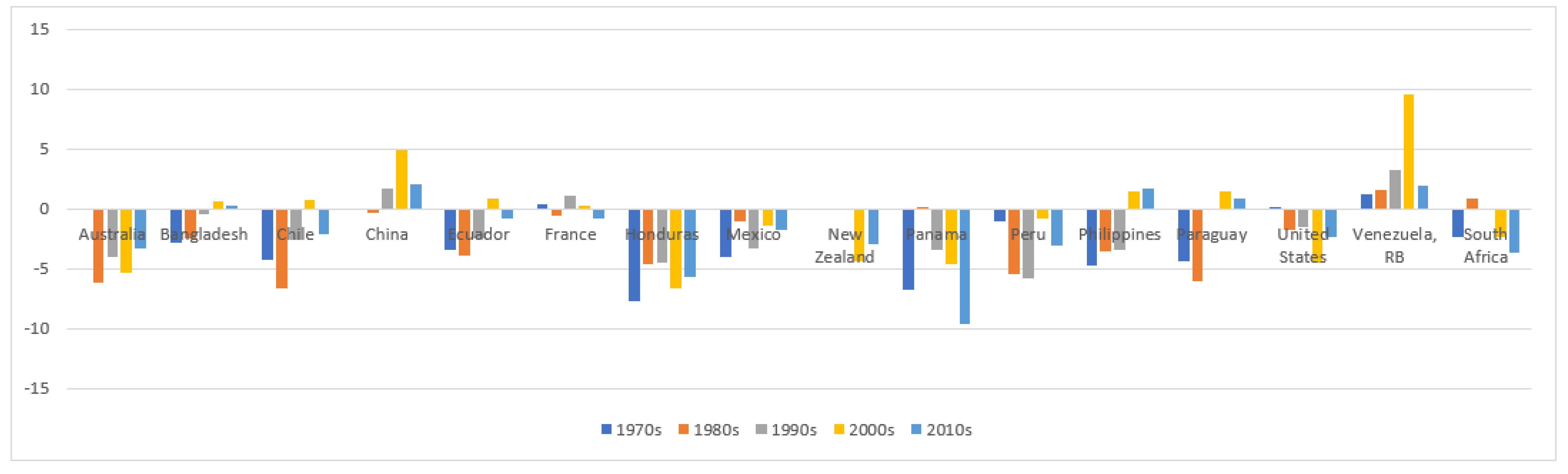
Finally, we turn our attention to the size of the slope coefficient relating to Equation (4). As noted in Section 2, apart from cointegration, the solvency condition relies on the size of the b (when statistically significant). We estimate the long run coefficient slope for those nations that have a cointegration relationship using the Full Modified OLS regression technique, which is suitable for cointegrated variables.11

Table 8. Regression (FMOLS) results for cointegrating variables: 1970–2018. This table reports the FMOLS results for countries that show a cointegration relationship between E and M over the period 1970–2018. The coefficient and the corresponding p-values relate to $b$ in Equation (3).

Variable	Coef.	Prob.	Adj.R2
Australia	0.894	0.000	0.836
C	1.052	0.430
Bangladesh	1.032	0.000	0.837
C	−7.319	0.000
Chile	1.481	0.000	0.697
C	−11.584	0.026
Ecuador	0.982	0.000	0.737
C	−0.927	0.026
Honduras	0.674	0.000	0.878
C	4.903	0.079
Mexico	0.880	0.000	0.916
C	1.771	0.223
New Zealand	0.640	0.003	0.217
C	10.481	0.078
Paraguay	1.362	0.000	0.855
C	−8.315	0.054
Venezuela	0.082	0.548	−0.019
C	26.430	0.000

and

Table 9. Regression (FMOLS) results for cointegrating variables: sub-analysis. This table reports the FMOLS results for countries that show a cointegration relationship between E and M in the sub-sample analysis. The first row shows the sub-samples. The coefficient and the corresponding p-values relate to $b$ in Equation (3).

1970–1999				1970–2004			1970–2009			1970–2014
	Coef.	Prob.	Adj R2	Coef.	Prob.	Adj R2	Coef.	Prob.	Adj R2	Coef.	Prob.	Adj R2
China				1.152	0.000	0.933	1.243	0.000	0.948	1.226	0.000	0.953
C				−0.910	0.307		−1.472	0.079		−1.386	0.095
Panama	0.653	0.000	0.946	0.656	0.000	0.944	0.693	0.000	0.904	0.736	0.000	0.901
C	15.129	0.000		14.978	0.000		13.173	0.000		10.434	0.008
Peru				1.032	0.003	0.096
C				−2.188	0.717
Philippines				0.821	0.000	0.925
C				2.406	0.236
South Africa	0.661	0.014	0.196
C	10.867	0.072

report these results for the sample period 1970–2018 and the sub-samples. We examine these results, together with average current account as a percentage of GDP over the most last two decades, which we present in Figure 1.

For Bangladesh, $b$ is equal to 1, and together with a long run cointegration relationship between E and M, these results suggest a strong form of sustainability of external balances. A few studies have noted that the current account of Bangladesh was unsustainable over the period 1960–2000 (Narayan and Narayan 2005); or weakly sustainable over the period 1982–2012 (Wadud et al. 2015). Indeed, Bangladesh’s current account deficits averaged over 2.0% in the 1970s and 1980s. However, over the last three decades, Bangladesh’s current account imbalances have improved; the average deficit fell to 0.45% in the 1990s; and averaged a positive 0.65% in the 2000s and only 0.22% in the 2010s. The low imbalances and the sharp decline in the average imbalances in the recent decade are consistent with our result that the nation’s current account follows a sustainable path.

The size of b is close to zero for Australia, Ecuador, Honduras, Mexico, New Zealand, and Venezuela, which also showed a cointegration relationship between E and M. The overall finding for these countries is that their current account shows the weak form of sustainability. Australia’s current account imbalances as a percentage of GDP averaged −6.12% and −4.08% in the 1980s and 1990s, respectively. The average deficit as a percentage of GDP fell to 3.29% in the 2010s, from the levels (5.30%) reached in the 2000s. Australia’s current account needed to attain some positive imbalances to attain the strong form of sustainability.

Ecuador’s large deficits in the 1970s to 1990s (ranging from 3.86% to 2.44%) overshadow the lower average imbalances in the last two decades, which explains its weak form of unsustainability. Ecuador’s policymakers need to push the imbalances into the positive zone and improve its sustainability with a more vigorous policy effort.

Honduras shows average deficits, ranging from 4.46% (1990s) to 7.67% (1970s). Honduras is strongly dependent on trade. Exports and imports of goods and services together account for more than 92% of its GDP, the highest out of the 16 cases (Table 1). The annual data on the current account from the World Bank database12 reveal reversal of the current account. We note repeated patterns of reversal of the current account imbalances lasting one to four years, following a big jump in the imbalances over the period 1980–2018. The current account imbalances were increasing (declining) in the years preceding (following) the high deficit levels of 1980, 1984, 1994, 1996, 2000, 2004, 2008, 2013, and 2018. Hence, while the current account was full reversals, the average growth of exports was slower than imports and, as a result, Honduras was only weakly satisfying its solvency condition. To be on a sustainable path the nation needed to increase growth of exports and/or reduce growth of imports.

For Mexico, while the current account was, on average, always in deficit, this was higher in the 1970s (averaging 4.02% of GDP) and the 1990s (averaging 3.26% of GDP) than in other decades. Over the period 1970 to 2018 Mexico would have needed to push for current account surpluses in some years to achieve the strong form of sustainability.

For New Zealand, comparable current account data is available for the last two decades and they fell only slightly to an average of 2.93% in the 2010s from the 2000s average of 4.41%. Finally, for Venezuela, a sharp growth in the current account imbalances in the 2000s (9.56% of GDP) overshadowed the low and slow growing average current account surpluses in the 1970s–1990s (1.99%) and 2010s (1.90%). While the average imbalances in the most recent decade (2010) improved significantly, falling below the 2000s average level, these improvements fell short of taking the Venezuelan current account to more solid ground.

Both Chile and Paraguay show a cointegration relationship between exports and imports, but since they present a case where b is greater than 1, they are at odds with the solvency condition, which shows that their current accounts are unsustainable. Unreported results over the sub-sample periods for Chile and Paraguay suggest that b is always greater than 1.13 For both countries in most years, our slope results seem to be at odds with the average current account imbalances in Figure 1. This is due to the fact that, on average, net direct transfer and income in these countries contribute more to the current account than net trade.

From the sub-sample results reported in Table 9, we learn that China always showed the strong form of sustainability between all sub-samples in the period 1970–2014, except with the most recent five years of data. While the average current account surplus in the most recent decade (2010s) fell to 2.04% from the average of 4.96% in the decade earlier (2000s), China has not been able to fully reverse the persistently large surpluses of the 2000s.

On the other hand, Panama’s current account was weakly sustainable up to 2009. There is a cointegration relationship between exports and imports up to the period 1970–2009, and the size of b is significant, but less than one. This is not surprising considering its current account deficit registered an average of 9.56% of GDP in the decade starting 2010, the highest of all countries in that decade.

With the size of b being significant, but less than one, Peru, and South Africa showed weak case of sustainability intermittently: South Africa over 1970–1999, and for Peru over the period 1970–2004. These results align well with current account data. Peru ran large deficits on average in the 1980s, 1990s and 2010s, while South Africa saw large growths in deficits in the last two decades. Again, these nations need more focused and long-term policies to have more sustainability in their current accounts.

Apart from these countries, France, the Philippines, and the United States showed no sign of cointegration over all sub-samples. For the Philippines, there were large deficits in the 1970s–1990s, while for the US, the persistently large deficits of the 2000s have contributed to these results. Compared to other countries, France, on the other hand, had low average current account imbalances as a percentage of GDP. Nonetheless, France’s intertemporal solvency condition was not satisfied, or the long run equilibrium relationship was not evident because the accumulated surpluses in the 1970s, 1990s, and 2000s saw no sufficient reversal over the study period.

6. Conclusions

This paper examined the sustainability, over the period 1970–2018, of the current accounts of 16 nations within the framework of intertemporal solvency theory. This theory implies that a strong form current account sustainability exists when exports and imports are cointegrated, and exports and imports grow proportionately. We conducted cointegration test of exports (E) and imports (M) of goods and services as a ratio of GDP (%) with and without breaks and estimated the size of the b for countries that showed cointegration. Our results showed that the current account of Bangladesh is sustainable in the strong form. For six out of the 16 countries, namely Australia, Ecuador, Honduras, Mexico, New Zealand, and Venezuela, we find a case for the weak form of sustainability, where E and M are cointegrated, but b is less than 1. Chile and Paraguay, on the other hand, are cointegrated, but b is greater than 1. The current accounts of these two countries are unsustainable.

Our sub-sample analysis for some countries that did not show cointegration over the period 1970–2018 showed cointegration intermittently over the period 1970–2018. Two other countries, Peru and South Africa, showed a weak form of sustainability intermittently over at least one sub-sample period. Panama showed current account unsustainability after 2009 and the weak form of sustainability over the period 1970–2009. China, on the other hand, showed a strong form of sustainability between all sub-samples in the period 1970–2014, making an exception of the sample of the most recent five years of data. France, the Philippines, and the United States unequivocally failed the intertemporal solvency test over the period 1970–2018.

Our study reveals that most countries are facing policy challenges around current account sustainability. As indicated in Section 1, the solvency test used here is one of several methods for measuring current account sustainability. Further, while we apply structural break dates and indicate when some current accounts switched to an unsustainable path, we do not explicitly study the current account shocks that trigger these changes. Future research endeavours on the topic may take two directions: (1) exploring additional methods to evaluate current account sustainability; and (2) examining the current account determinants to providing a better understanding of contemporary current account shocks. As demonstrated in this paper, both these research directions would make a vital contribution to modern-day policymaking.

References

- Baharumshah, Ahmad Zubaidi, Evan Lau, and Stilianos Fountas. 2003. On the sustainability of current account deficits: Evidence from four ASEAN countries. Journal of Asian Economics 14: 465–87. [Google Scholar] [CrossRef]
- Bohn, Henning. 2007. Are stationary and cointegration restrictions really necessary for the intertemporal budget constraint? Journal of Monetary Economics 54: 1837–47. [Google Scholar] [CrossRef]
- Chen, Shyh-Wei, and Zixiong Xie. 2015. Testing for current account sustainability under assumptions of smooth break and nonlinearity. International Review of Economics and Finance 38: 142–56. [Google Scholar] [CrossRef]
- Christopoulos, Dimitris, and Miguel León-Ledesma. 2010. Current account sustainability in the US: What did we really know about it? Journal of International Money and Finance 29: 442–59. [Google Scholar] [CrossRef]
- Cipollini, Andrea. 2002. Testing for Government intertemporal solvency: A smooth transition error correction model approach. The Manchester School 69: 643–55. [Google Scholar] [CrossRef]
- Corden, Warner Max. 1994. Economic Policy, Exchange Rates and the International Systems. Oxford: Oxford University Press. [Google Scholar]
- Cuestas, Juan Carlos. 2013. The Current account sustainability of European transition Economies. Journal of Common Market Studies 51: 232–45. [Google Scholar] [CrossRef]
- Cunado, Juncal, Luis Gil-Alana, and Fernando Pèrez de Gracia. 2010. European current account sustainability: New evidence based on unit roots and fractional integration. Eastern Economic Journal 36: 177–87. [Google Scholar] [CrossRef]
- Edwards, Sebastian. 2004. Financial openness, sudden stops and current-account reversals. American Economic Review American Economic Association 94: 59–64. [Google Scholar] [CrossRef] [Green Version]
- Engler, Philipp, Michael Fidora, and Christian Thiman. 2009. External imbalances and the US current account: How supply-side changes affect an exchange rate adjustment. Review of International Economics 17: 927–41. [Google Scholar] [CrossRef] [Green Version]
- Fischer, Stanley. 2003. Financial crisis and reform of the international financial systems. Review of World Economies 139: 1–37. [Google Scholar] [CrossRef] [Green Version]
- Giles, David E., and Ryan T. Godwin. 2012. Testing for multivariate cointegration in the presence of structural breaks: p-values and critical values. Applied Economics Letters 19: 1561–65. [Google Scholar] [CrossRef] [Green Version]
- Gnimassoun, Blaise, and Issiaka Coulibaly. 2014. Current account sustainability in Sub-Saharan Africa: Does the exchange rate regime matter? Economic Modelling 40: 208–26. [Google Scholar] [CrossRef] [Green Version]
- Greenidge, Kevin, Carlos Holder, and Alvon Moore. 2011. Current account deficit sustainability: The case of Barbados. Applied Economics 43: 973–84. [Google Scholar] [CrossRef]
- Hakkio, Craig S., and Mark Rush. 1991. Is the budget deficit too large? Economic Inquiry 29: 429–45. [Google Scholar] [CrossRef]
- Hassan, Kamrul, Ananth Rao, and Ariful Hoque. 2016. Current account sustainability in Middle East and Africa (MEA) countries: Evidence from panel data. The Journal of Developing Areas 50: 291–304. [Google Scholar] [CrossRef] [Green Version]
- Holmes, Mark J., Theodore Panagiotidis, and Abhijit Sharma. 2011. The sustainability of India’s current account. Applied Economics 43: 219–29. [Google Scholar] [CrossRef]
- Husted, Steven. 1992. The emerging US current account deficit in the 1980s: A cointegration analysis. Review of Economics and Statistics 74: 159–66. [Google Scholar] [CrossRef]
- Ismail, Hamizun Bin, and Ahmad Zubaidi Baharumshah. 2008. Malaysia’s current account deficits: An intertemporal optimization perspective. Empirical Economics 35: 569–90. [Google Scholar] [CrossRef] [Green Version]
- Jácome, Luis Ignacio. 2004. The Late 1990s Financial Crisis in Ecuador: Institutional Weaknesses, Fiscal Rigidities, and Financial Dollarization at Work, IMF Working Paper, WP/04/12. Available online: https://www.imf.org/external/pubs/ft/wp/2004/wp0412.pdf (accessed on 8 July 2020).
- Johansen, Søren, Rocco Mosconi, and Bent Nielsen. 2000. Cointegration analysis in the presence of structural breaks in the deterministic trend. Econometrics Journal 3: 216–49. [Google Scholar] [CrossRef] [Green Version]
- Kaufmann, Sylvia, Johann Scharler, and Georg Winckler. 2002. The Austrian current account deficit: Driven by twin deficits or by intertemporal expenditure allocation? Empirical Economics 27: 529–42. [Google Scholar] [CrossRef]
- Kraay, Aart, and Jaume Ventura. 2002. Current Accounts in the Long Run and the Short Run. NBER Working Papers 9030. Cambridge: National Bureau of Economic Research. [Google Scholar]
- Leachman, Lori, and Michael Thorpe. 1998. Intertemporal solvency in the small open economy of Australia. The Economic Record 74: 231–42. [Google Scholar] [CrossRef]
- Lees, Francis A. 2007. The Mexican financial crisis. International Journal of Public Administration 23: 877–906. [Google Scholar] [CrossRef]
- Liu, Peter C, and Evan Tanner. 1996. International intertemporal solvency in industrialised countries: Evidence and implications. Southern Economic Journal 62: 739–49. [Google Scholar] [CrossRef]
- Makrydakis, Stelios. 1999. Consumption-smoothing and the excessiveness of Greece’s current account deficits. Empirical Economics 24: 183–209. [Google Scholar] [CrossRef]
- Milesi-Ferreti, Gian Maria, and Assaf Razin. 1996. Sustainability of Persistent Current Account Deficits. NBER Working Paper Series 5467. Cambridge: National Bureau of Economic Research. [Google Scholar]
- Milesi-Ferreti, Gian Maria, and Assaf Razin. 1998. Current Account Reversals and Currency Crisis: Empirical Regularities. NBER Working Papers 6620. Cambridge: National Bureau of Economic Research. [Google Scholar]
- Narayan, Paresh Kumar. 2005. The Saving and Investment Nexus for China: Evidence from Cointegration Tests. Applied Economics 37: 1979–90. [Google Scholar] [CrossRef]
- Narayan, Seema. 2009. A survey on dynamics of the current account imbalances. The Indian Economic Journal 57: 1–26. [Google Scholar] [CrossRef]
- Narayan, Seema. 2020. Asian current account balances and spillovers from a foreign country, a region and the United States. Bulletin of Monetary Economics and Banking 23: 1–24. [Google Scholar] [CrossRef]
- Narayan, Paresh Kumar, and Seema Narayan. 2004. Is there a long-run relationship between exports and imports? Evidence from two Pacific Island countries. Economic Papers 23: 152–64. [Google Scholar] [CrossRef]
- Narayan, Paresh Kumar, and Seema Narayan. 2005. Are exports and imports cointegrated? Evidence from 22 countries. Applied Economic Letters 12: 375–78. [Google Scholar] [CrossRef]
- Obstfeld, Maurice, and Kenneth Rogoff. 2000. Perspectives on OECD capital market integration: Implications for the US current account adjustments. In Global Economic Integration: Opportunities and Challenges. Kansas City: Federal Reserve Bank of Kansas City, pp. 169–208. [Google Scholar]
- Ogus, Ayla, and Niloufer Sohrabji. 2008. On the optimality and sustainability of Turkey’s current account. Empirical Economics 35: 543–63. [Google Scholar] [CrossRef]
- Önel, Gülcan, and Utku Utkulu. 2006. Modelling the long-run sustainability of Turkish external debt with structural changes. Economic Modelling 23: 669–82. [Google Scholar] [CrossRef]
- Pattichis, Charalambos. 2010. The intertemporal budget constraint and current account sustainability in Cyprus: Evidence and policy implications. Applied Economics 42: 463–73. [Google Scholar] [CrossRef]
- Perron, Pierre. 1989. The great crash, the oil price shock, and the unit root hypothesis. Econometrica 57: 1361–401. [Google Scholar] [CrossRef]
- Perron, Pierre. 1997. Further evidence on breaking trend functions in macroeconomic variables. Journal of Econometrics 80: 355–85. [Google Scholar] [CrossRef] [Green Version]
- Pesaran, M. Hashem, and Yongcheol Shin. 1999. An Autoregressive Distributed Lag Modelling Approach to Cointegration Analysis, Econometric and Economic Theory in the 20th Century: The Ragnar Frisch Centennial Symposium. Edited by S. Strom. Cambridge: Cambridge University Press. [Google Scholar]
- Philip, Peter C. B., and Bruce E. Hansen. 1990. Statistical Inference in instrumental variables regression with I(1) processes. Review of Economic Studies 57: 99–125. [Google Scholar] [CrossRef]
- Quintos, Carmela E. 1995. Sustainability of the deficit process with structural shifts. Journal of Business and Economics Statistics 13: 409–17. [Google Scholar]
- Rogoff, Kenneth. 2007. Global imbalances and exchange rate adjustment. Journal of Policy Modeling 29: 705–9. [Google Scholar] [CrossRef]
- Sachs, Jeffery D. 1981. The current account and macroeconomic adjustment in the 1970s. In Brooking Papers on Economic Activity. Washington, DC: Brookings Institution Press, pp. 201–68. [Google Scholar]
- Singh, Tarlok. 2015. Sustainability of current account deficit in India: An intertemporal perspective. Applied Economics 47: 4934–51. [Google Scholar] [CrossRef]
- Singh, Tarlok. 2019. Intertemporal sustainability of current account imbalances: New evidence from the OECD countries. Economic Notes 48: 1–40. [Google Scholar] [CrossRef]
- Ventura, Jaume. 2003. Towards a theory of current accounts. The World Economy 26: 483–512. [Google Scholar] [CrossRef] [Green Version]
- Wadud, Abdul, S. M. Atiar Rahman, and Mohammod Mozammel Hossain Chowdhury. 2015. Sustainability of the current account in Bangladesh: An intertemporal and cointegration analysis. The Journal of Developing Areas 49: 353–64. [Google Scholar] [CrossRef]
- Wickens, Michael R., and Merih Uctum. 1993. The sustainability of current account deficits. A test of the US intertemporal budget constraint. Journal of Economic Dynamics and Control 17: 423–41. [Google Scholar] [CrossRef]
- Yol, Marial A. 2009. Testing the sustainability of current account deficits in developing economies: Evidence from Egypt, Morocco and Tunisia. The Journal of Developing Areas 43: 177–97. [Google Scholar] [CrossRef]