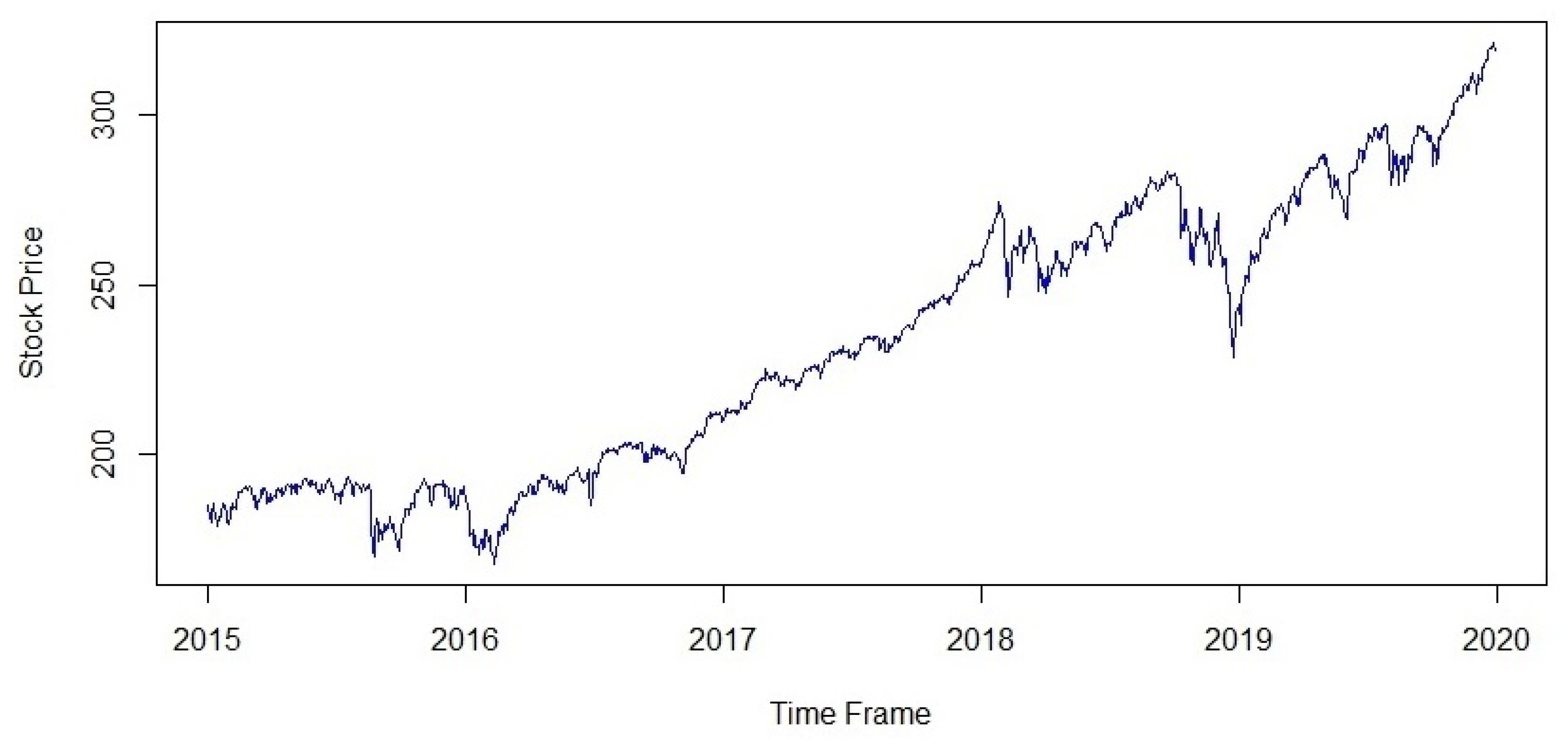
Article

Comparison of Financial Models for Stock Price Prediction

by
Mohammad Rafiqul Islam
and
Nguyet Nguyen
*
Department of Mathematics and Statistics, Youngstown State University, Youngstown, OH 44555, USA
*
Author to whom correspondence should be addressed.
J. Risk Financial Manag. 2020, 13(8), 181; https://doi.org/10.3390/jrfm13080181
Submission received: 30 July 2020 / Revised: 9 August 2020 / Accepted: 12 August 2020 / Published: 14 August 2020
(This article belongs to the Special Issue Mathematical Finance with Applications)

Abstract

:
Time series analysis of daily stock data and building predictive models are complicated. This paper presents a comparative study for stock price prediction using three different methods, namely autoregressive integrated moving average, artificial neural network, and stochastic process-geometric Brownian motion. Each of the methods is used to build predictive models using historical stock data collected from Yahoo Finance. Finally, output from each of the models is compared to the actual stock price. Empirical results show that the conventional statistical model and the stochastic model provide better approximation for next-day stock price prediction compared to the neural network model.

1. Introduction

Predicting modeling is one of the most popular mathematical methods in many fields such as business, social science, engineering, and finance. In business, predictive modeling is also known as predictive analytics. Among many, one of the most important applications of predictive modeling is to predict the stock price. Modern predictive modeling can be categorized into two basic categories such as statistical and soft computing techniques (Adebiyi et al. 2014). Autoregressive integrated moving average (ARIMA) is one of the most popular and widely used statistical techniques for making predictions using past observations (Meyler et al. 1998). In spite of having great popularity in making predictions, this method has some limitations such as seasonality, non-stationarity, and other factors (Tambi 2005). In contrast, as a machine learning method or soft computing technique, artificial neural networks (ANNs) are one of the most accurate and widely used forecasting models for forecasting, pattern recognition, and image processing (Khashei and Bijari 2010). Neural network models have become more popular in forecasting over the last decade in business, economics, and finance (Avcı 2007). According to Khashei and Bijari (2010), ANNs are distinguished and most effective for predictive modeling because of their data-driven self-adaptive nature and they are universal function approximators. The network can generalize, this means that once the network learns the data, it can predict the unseen or future part of the data even if the given data is not smooth.
In addition to the above two methods, stochastic modeling that uses geometric Brownian motion to predict the stock price is very popular. Brownian motion is a special type of motion of molecular particles, first observed and described by the British-Scottish botanist in 1827. However, Louis Bachelier, a French mathematician named this Brownian motion and proposed a model to predict stock prices using Brownian motion in 1900. According to the geometric Brownian motion model, the returns on a certain stock in successive, equal periods of time are independents and normally distributed (Dmouj 2006). The equation of geometric Brownian motion has a constant volatility and drift, but in real-world scenario these are not constant and vary over time (Estember and Maraña 2016). Hence, we consider time variant volatility and drift in our analysis.
There are many researchers using the three basic techniques: ARIMA, ANN, and stochastic models to predict stock prices, which will be reviewed in the next section. However, in the literature, there are no comparisons of using each of the three models to predict prices of one stock. Most of the researchers compared performances of the two models ARIMA and ANN in stock price predictions, but not all of the three methods. Therefore, in this paper, we build predictive models using all of the above three modeling techniques and compare the models’ performance for stock price predictions, which are discussed in the subsequent sections. Section 2 represents the literature review and related works. In Section 3, we describe the general theories for each of the methods and then build the models specifically for S & P 500 index. In Section 4, we describe the results from each of the three models and model diagnostics. Section 5 contains the conclusions.

2. Literature Review

Prediction has long been a popular field in mathematical science, so there is plenty of related research in the field. The first significant study of neural network models for stock price prediction was done by (White 1988). His predictive model was based on IBM’s daily common stock and the training predictions were very optimistic. Thereafter, a lot of research was performed to check the neural networks’ accuracy of prediction to forecast the stock market. Hassan et al. (2007) proposed a fusion model by combining the hidden Markov model (HMM), artificial neural network (ANN), and genetic algorithms (GA) to forecast financial market behavior. They found that the performance of the fusion tool is better than that of the basic model (Hassan and Nath 2005) where they used only a single HMM. They also indicated that the performance of the fusion model is similar to that of the ARIMA model. Zhang and Wu (2009) proposed an integrated model improved bacterial chemotaxis optimization (IBCO) and back propagation artificial neural network to predict the S & P 500 index. The IBCO based back propagation (or IBCO-BP) model is less computationally complex and has better accuracy. Khashei and Bijari (2010) found that the performance of a neural network for some real time series is not satisfactory. Hence, using ARIMA models, they suggested a novel hybrid type of artificial neural network. The proposed model provided better predictions for three separate actual datasets than just the neural artificial network model. Yao et al. (1999) compared the back propagation neural network model and ARIMA model stock index forecasting. They found that the neural network results in better accuracy in forecasting than the traditional ARIMA models. Adebiyi et al. (2014) compared the forecasting performance by ARIMA and artificial neural network for stock data. They analyzed daily stock prices for the Dell Incorporation and found a superiority of the neural network model over the ARIMA model.
Merh et al. (2010) developed a three-layer feed-forward neural network model and auto-regressive integrated moving average model to predict the future value of the stock price and revealed that the ARIMA models perform better over ANN models. Lee et al. (2007) did a comparative study of the forecasting performance by neural network models and the time series model (SARIMA) for the Korean Stock Index data. They also found ARIMA models outperforming ANN models for the stock price prediction. Agustini et al. (2018) used several stock indexes under the Jakarta Corporate Index to build a predictive model with Brownian motion. They found a higher accuracy for prediction with a mean absolute percentage error (MAPE) less than 20%. Rathnayaka et al. (2014) developed a forecasting model using the geometric Brownian motion model and compared the predictions with the results from the traditional time series model ARIMA. They used the Colombo Stock Exchange (CSE), Sri Lanka data to build their models and found that the stochastic model prediction is more significant than the traditional model.
The literature shows different opinions on the relative performances of the two of the three models depending on data. Hence, further comparative studies of all the three models can assemble a consistent methodology for stock price prediction. In this paper, we study the comparative performances of the three models in predicting next-day stock prices for S & P 500 index data from Yahoo Finance.

3. Methodology

The methodology section contains the basic four subsections. The first subsection describes the data that were used to build the models. Then, each of the subsections describes general theories and procedures to build the models and then how the models were fitted for a particular dataset. The overall performance of each of the models was checked by the analysis of the residuals and four different error measures, namely the absolute percentage error (APE), the average absolute error (AAE), the average relative percentage error (ARPE), and the root-mean-square error (RMSE) (Nguyet Nguyen and Wakefield 2018). The formula to calculate these errors are as follows:
A P E = 1 r ¯ i = 1 N r i r ¯ i N , A E E = i = 1 N r i r ¯ i N , A R P E = 1 N i = 1 N r i r ¯ i N , R M S E = 1 N i = 1 N r i r ¯ i N .

3.1. Data

S & P 500 daily stock for the period 1 January 2015 to 31 December 2019 was used in this research. We used the quantmod package (Ryan et al. 2020) in statistical software R, version 1.2.1335 to collect the data directly from Yahoo Finance. Initially, the dataset contains six variables, namely daily Open, High, Low, Close, Volume, and Adjusted Close price. Addition to the six variables, we created two more variables, i.e., Average and Return. The Average variable is the average of daily Open, High, Low, and Close price. All the predictive models were built to predict the Adjusted Close price for the next day on the basis of the present day’s predictor variables. There were 63 trading days per quarter in 2019. All the models were used to predict the next-day stock price for the last quarter of 2019. A total of 63 predictions were made.

3.2. Autoregressive Integrated Moving Average Process

3.2.1. ARIMA(p,d,q) Models

The time series analysis requires the stationarity of the data, meaning the statistical properties such as mean, variance, and so on do not change over time. However, most of the real-world data, like stock data, are non-stationary by nature. This non-stationarity can be taken care of by using the Box–Jenkins ARIMA(p,d,q) approach (Makridakis and Hibon 1997). A time series { Y t } is said to follow an Autoregessive Integrated Moving Average ARIMA(p,d,q) if the dth difference W t = d Y t is a stationary A R M A ( p , q ) process (Cryer and Kellet 1991). A generalised A R I M A ( p , d , q ) model can be written as
W t = ϕ 1 W t 1 + ϕ 2 W t 2 + + ϕ p W t p + e t + θ 1 e t 1 + θ 2 e t 2 + + θ q e t q ,
where ϕ 1 , ϕ 2 , , ϕ p and θ 1 , θ 2 , , θ q are the autoregressive and moving average parameters, respectively, and e s are the white noise. The autoregression A R ( p ) , order p, and moving average M A ( q ) , order q, are determined from the analysis of the autocorrelation function. The number d indicates the number of differences applied to the time series to remove the trend. The autoregressive parameters ϕ s and moving average parameters θ s are estimated from the model based on p , d , and q .

3.2.2. ARIMA(p,d,q) Model for S & P 500 Index

The adjusted close price of S & P 500 is a time series process { X t } that has been analysed to build the model. The process { X t } is not a stationary process, if we see the following graphs.
Figure 1 shows an upward trend in the data. Inspecting the sample autocorrelation plot from Figure 2, it is clear that the Auto Correlation Function (ACF) dies down very slowly and the Partial Autocorrelation Function (PACF) cuts off at lag 1 with correlation one.
The slow dying-down nature of the ACF indicates that the process is non-volatile. That is, the current value is relating with all the past values. These facts ensure the process is non stationary. To make the process stationary, we transform the { X t } series to the { Y t } = { log X t } series and then to a new series { W t } = { 2 Y t } , where W t = Y t 2 Y t 1 + Y t 2 .
Figure 3 is the window plot of the second differenced log transformed stock price. From this plot, the data looks stationary and randomized. Stationarity has been confirmed from the augmented Dickey–Fuller test (Cheung and Lai 1995) with a p value of 0.01 , where the alternative hypothesis was stationary. Next, the autoregressive and moving average orders p and q were determined from the PACF and ACF plot from Figure 4.
The ACF cuts of at lag 1 which indicates that the process incorporates an M A process of order q = 1 whereas the PACF gradually dies down. Therefore, the series W t follows an M A ( 1 ) process or the series Y t follows an I M A ( 2 , 1 ) process i.e. Y t A R I M A ( 0 , 2 , 1 ) . Other A R I M A ( p , d , q ) models were also considered in this research, as shown in Table 1. The best model has been chosen based on the Schwarz Bayesian Information Criterion (BIC) (Neath and Cavanaugh 2012) criteria, the more negative, the more accurate model. The reason of not choosing Akaike Information Criterion (AIC) or Bias Corrected Akaike Information Criterion (AICc) is that those models provide over-fitting and non significant parameters.
From Table 1, the A R I M A ( 0 , 2 , 1 ) model has the most negative BIC value which fits the data most perfectly. The Arima function with order ( p , d , q ) = ( 0 , 2 , 1 ) was run in RStudio and the summary of the model is displayed in Table 2.
The model in difference equation is given as
W t = e t + θ e t 1 2 Y t = e t + θ e t 1 Y t 2 Y t 1 + Y t 2 = e t + θ e t 1 Y t = 2 Y t 1 Y t 2 + e t + θ e t 1 .
Finally, substituting the MA parameter θ = 1 in Equation (2), the model for Y t = log X t is given as
Y t = 2 Y t 1 Y t 2 + e t e t 1 .
A fixed window of 1194 past observed stock prices have been used to predict each of the next-day prices using the model in Equation (3). Hence, the training dataset moved and the end price of the window was updated with the actual price. The results and diagnostics of this model are discussed in Section 4.1.

3.3. Stochastic Model Geometric Brownian Motion

A process that generates some outcomes which are time-dependent but can not be said ahead of time is known as a stochastic process. A stochastic process { W ( t ) : 0 t T } is a standard Brownian motion on [ 0 , T ] if
  • W ( 0 ) = 0
  • It has independent increments. That is, for any t 1 , t 2 , , t n , W ( t 2 ) W ( t 1 ) , W ( t 3 ) W ( t 4 ) , W ( t n ) W ( t n ) are independent random variables.
  • For every 0 s < t T , W ( t ) W ( s ) ( 0 , t s ) .
A stochastic process { X ( t ) : 0 < t < T } is said to be a general Brownian motion with a drift parameter μ and diffusion coefficient σ 2 if X ( t ) μ t σ is a standard Brownian motion, written as X ( t ) B M ( μ , σ 2 ) .
The general Brownian motion still follows first two properties of the standard Brownian motion. However, the third property is modified as X ( t ) X ( s ) ( μ ( t s ) , σ 2 ( t s ) ) for any 0 s < t < T .

3.3.1. Geometric Brownian Motion (GBM) Model

If X ( t ) B M ( μ , σ 2 ) then X ( t ) satisfies the stochastic differential equation (Yang and Aldous 2015)
d X ( t ) = μ t + σ d W ( t ) ,
where, W ( t ) is the standard Brownian motion or Wiener process. If the stochastic process is defined as X ( t ) = log S ( t ) then d S ( t ) = μ S ( t ) d t + σ S ( t ) d W ( t ) is the stochastic differential equation for the stock price random process.
For a given time t > 0 , the standard model for stock prediction can be given from the stochastic differential equation by integration
S ( t ) = S ( 0 ) + μ 0 t S ( r ) d r + σ 0 t S ( r ) d W ( r ) .
A more explicit formula can be derived using Ito’s formula (Ševcovic et al. 2011) to the function F ( log S ( t ) , t )
d F = F t + μ F S ( t ) + 1 2 σ 2 2 F 2 S ( t ) d t + σ F S ( t ) d W ( t ) ,
which results
d log S ( t ) = 1 S ( t ) d S ( t ) + 1 2 1 S 2 ( t ) ( d S ( t ) ) 2 = μ d t + σ d W ( t ) + 1 2 1 S 2 ( t ) ( μ S ( t ) d t + σ S ( t ) d W ( t ) ) 2 = ( μ 1 2 σ 2 ) d t + σ d W ( t ) .
For any time t > 0 , the differential can be written as
log S ( t ) = log S ( 0 ) + ( μ 1 2 σ 2 ) t + σ W ( t ) Or , S ( t ) = S ( 0 ) e ( μ 1 2 σ 2 ) t + σ W ( t ) .

3.3.2. Geometric Brownian Motion Model for S & P 500 Index: GBM( μ , σ 2 ) Simulation

For a given time set, t 0 = 0 < t 1 < t 2 < < t n , the stock price S ( t ) at time t 0 , t 1 , , t n can be generated by
S ( t i + 1 ) = S ( t i ) e ( μ 1 2 σ 2 ) ( t i + 1 t i ) + σ ( t i + 1 t i ) Z i + 1 ,
where Z 1 , Z 2 , Z n are independent and identically distributed standard normals and i = 0 , ( n 1 ) ¯ . In our case, the time interval t i + 1 t i = 1 for all i = 0 , ( n 1 ) ¯ , since we are predicting the next-day price. Hence, the model becomes
S ( t i + 1 ) = S ( t i ) e ( μ 1 2 σ 2 ) + σ Z i + 1 .
Using the model in Equation (8), we simulate a large number of prices, and from that we take the average to predict the next-day price. For our data, this large number is 100,000 . A total of 63 predictions have been made using this model. A fixed window of 1194 past observed stock prices have been used to predict each of the next-day prices. Hence, the training dataset moved, and the end price of the window was updated with the actual price. The results and diagnostics of this model are discussed in Section 4.2.

3.4. Artificial Neural Network

This section describes how an artificial neural network can be used to predict the stock price and how to build a model based on the stock data for S & P 500 index.

3.4.1. Model Descriptions

Artificial neural network is one of the most popular machine learning techniques for nonlinear approximations because of its ability to deal with a large number of functions with a high degree of accuracy (Chen et al. 2003). The idea of ANN came from the structure of the animal brain, more specifically, from the human neural system. It is based on the idea of how brain works, how the neurons in the brain receive information from the input neurons, analyse it, and finally identify the object or pattern. Fundamentally, the mechanism has three layers—input layer, hidden layers, and output layer. Each layer consists of neurons or nodes. The hidden part may consist of many layers, however, for the time series analysis and forecasting, the single hidden layer feed forward network is the most widely used model structure (Zhang et al. 1998). A simple three layer neural network has the following mathematical form
Y t = W 0 + j = 1 q W j . g ( W 0 , j + i = 1 p W i , j . Y t i ) + ϵ t ,
where, W i , j and W j for i = 1 , 2 , , p , j = 1 , 2 , , q are known as connection weights. The parameter p and q are the number of input and output nodes respectively. The network involves an activation function which plays a very important role because it converts the input signals to be used for the neurons or nodes in the next layer, eventually the output neuron. The most widely used activation functions are the logistic and hyperbolic functions (Khashei and Bijari 2010), which are shown in Equations (10) and (11)
s i g ( x ) = 1 1 e x
tan 1 ( x ) = 1 e 2 x 1 + e 2 x .
Most of the modelers prefer the hyperbolic tangent function as the activation functions because of its faster convergence, and it makes the optimization easier. Hence, we used this activation function in our model. There is no systematic rule of choosing the number of neurons or nodes, q in the hidden layer (Khashei and Bijari 2010). In most of the cases it is data-dependent and chosen on the basis of trial and error.

3.4.2. Artificial Neural Network for S & P 500 Index

The model proposed for S & P 500 in this section is a three layer model—input, hidden, and the output layer. The input layer consists of a total of seven nodes which are daily Open, Close, High, Low, Average, Volume, and Return. The variable Average is the average of daily Open, Close, High, and Low. The Volume was converted to million units. Daily return was calculated by this formula r t = log S t S t 1 , where S t is the adjusted closed price and day one return, r 0 was considered zero. The output layer has only one node that corresponds to the predicting variable Adjusted Close price. The number of the nodes in the hidden layer was chosen based on the error measures in Equation (1) for different combinations of the hidden nodes, which are displayed in Table 3. From this Table 3, we see that model ANN(7-15-1) has the lowest APE, AAE, ARPE, and RMSE and the highest adjusted R 2 value.
The original dataset had 1257 observations, but the dataset used in this method was modified in this way—all the predictor and predicting variables have the same length of 1256, however, the predictor variables started from day 1 to the 1256th day and the predicting variable day 2 to the 1257th day. Then, the dataset was divided into two parts to run the model. The test dataset contained the last 63 actual stock prices (adjusted close) which were compared to the predicted prices. The best model was selected on the basis of the adjusted R 2 and four error measures (Table 3). The model architecture is shown in Figure 5 and the result of this model is discussed in Section 4.3.

4. Results

In this section, the result of from the above three models is discussed and a window of the predicted and actual price is shown together with a graphical presentation. Finally, we assess how our model is performing by model diagnostics.

4.1. Autoregressive Integrated Moving Average

4.1.1. ARIMA Model Result

The model A R I M A ( 0 , 2 , 1 ) in Equation (3) produces the prediction in a logarithmic scale, which is then converted back to the original scale by the formula Predicted Price = e p r e d i c t i o n . Total 63 trading days have been predicted by the model and compared with the actual prices which has been shown in Table 4 with individual prediction error calculated by the formula,
error = actual predicted actual × 100 .
From Table 4, we see that the forecast errors are less than one dollar for the daily period from 12 November, 2019 to 30 December 2019, with the relative errors within the range of 0.00003 to 0.00292 . Figure 6 shows the graphical representation of the actual and predicted stock price by the model. The black line represents the actual stock price and the red line represents the predicted stock price for S & P 500. Figure 6 also shows that the ARIMA (0,2,1) predicted prices follow closely to the trend of the actual prices.

4.1.2. ARIMA Model Diagnostics

The performance of the ARIMA(0,2,1) model was assessed by the analysis of the four error measures state in Equation (1) and the residuals plot, which is depicted in Figure 7 and those four error measures are tabulated in Table 5.
From the results in Table 5, we see that all the error measures are comparatively very low to the actual prices, this indicates that the model is performing better in its prediction. From Figure 7 it is clear that the residuals do not follow any special pattern, they are a randomized plot. Correlations in the few lags are significant. Overall, the model fits very well to predict the stock price.

4.2. Stochastic Model

4.2.1. Stochastic Model Result

The model proposed in Equation (8) requires the calculation of 63 distinct values of the means μ and standard deviations σ of the daily returns. Both of the parameters were calculated on the basis of the same number of returns each time. Predicted values, actual values, and individual errors are shown in Table 6, and the errors were calculated by the same formula (12) used in the previous model. The results in Table 5 and Table 6 are almost the same except at some points. Thus, Figure 7 and Figure 8 are almost identical.
Figure 8 displays the graphical representation of the actual and predicted stock prices from the stochastic model. The black line represents the actual stock price and the green line represents the predicted stock price for S & P 500 index.

4.2.2. Stochastic Model Diagnostics

The performance of the stochastic model was assessed by the analysis of the four error measures stated in Equation (1) and the residual plot which is depicted in Figure 9 and the calculation of the four different error measures, as shown in Table 7.
The standardized residual plot is random and the mean passes through the zero line. A few of the residuals at the lower end are outside of the band in the Q-Q plot of the residuals. Still, both of the plots depict the approximate normal behavior of the residuals.

4.3. Artificial Neural Network

4.3.1. ANN(7-15-1) Results

Both of the training and test datasets were converted to normal and the prediction was converted back to the original scale by inverse transformation. The model required approximately 7000 steps with an error of 0.1972. Actual prices, predicted prices, and the corresponding errors are displayed in Table 8.
The predicted errors in Table 8 are much higher than those in Table 5 and Table 6. Precise comparisons of the three models are given in the next section. The graph associated with this result is displayed in Figure 10. The black line represents the actual stock price and the blue line represents the predicted stock price for the S & P 500 index. From the graph, it is clear that the model is working better at the beginning of the prediction interval.

4.3.2. ANN(7-15-1) Model Diagnostics

The performance of the neural network ANN(7-15-1) was assessed by the analysis of the four error measures stated in Equation (1) and the standardized residuals plot, which is depicted in Figure 11, and the calculation of the four different error measures are shown in Table 9.
The standardized residual plot does not show normal behavior. The error increases in an exponential shape as the predicting interval increases.

4.4. Comparison

In this section, the combined output from the three models above is discussed. Table 10 shows a sample of the empirical results obtained from the models and Figure 12 displays the result graphically.
From Figure 12 it clear that that ARIMA(0,2,1) model’s output and GBM model’s output are very close, sometimes they coincide, whereas the output from the ANN(7-15-1) model gets far from the actual points as time increases.
Looking at the error measures in Table 11, it is clear that the ARIMA model and stochastic model perform better than the neural network model for predicting the next-day stock price.

5. Conclusions

This study represents a comparative study of three financial models ARIMA, ANN, and Geometric Brownian Motion to predict the next-day stock prices. Results obtained from the analysis of the S & P 500 index show that the conventional statistical model ARIMA and the stochastic model-geometric Brownian motion model perform better than the artificial neural network models for short term next-day stock price prediction. The results are in contradiction with the results in Khashei and Bijari (2010), which concluded that the ARIMA was no better than the ANN model in time series predictions. However, their proposed hybrid ANN model outperformed the traditional ANN and the ARIMA models. Furthermore, our results are similar to the conclusions in Merh et al. (2010) and Lee et al. (2007) which stated that ARIMA models outperform ANN models for stock price predictions. On the other hand, Rathnayaka et al. (2014) found that the stochastic model prediction is more significant than the traditional ARIMA model. In fact, on the basis of our results, the ARIMA model and the stochastic model produce almost the same results. Thus, for short term prediction using the time series data, the ARIMA model and the stochastic model can be used interchangeably. For the ANN models, further studies, hybridization of existing models, and adding more independent variables can improve the neural network models in predicting stock prices. One model can work better than other models with particular time series data. Therefore, researchers or investors should examine some different models to predict the prices of each stock to find the best prediction model.

Author Contributions

M.R.I. setup and ran models, processed data, and wrote the first draft. N.N. introduced the methodology, refined the manuscript, and supervised the project. All authors have read and agreed to the published version of the manuscript.

Funding

This research received no external funding.

Conflicts of Interest

The authors declare no conflict of interest.

References

  1. Adebiyi, Ayodele Ariyo, Aderemi Oluyinka Adewumi, and Charles Korede Ayo. 2014. Comparison of arima and artificial neural networks models for stock price prediction. Journal of Applied Mathematics 2014: 614342. [Google Scholar] [CrossRef] [Green Version]
  2. Agustini, W. Farida, Ika Restu Affianti, and Endah R. M. Putri. 2018. Stock price prediction using geometric brownian motion. Journal of Physics: Conference Series 974: 012047. [Google Scholar]
  3. Avcı, Emin. 2007. Forecasting daily and sessional returns of the ise-100 index with neural network models. Dogus Universitesi Dergisi 8: 128–42. [Google Scholar] [CrossRef]
  4. Chen, An-Sing, Mark T. Leung, and Hazem Daouk. 2003. Application of neural networks to an emerging financial market: Forecasting and trading the taiwan stock index. Computers & Operations Research 30: 901–23. [Google Scholar]
  5. Cheung, Yin-Wong, and Kon S. Lai. 1995. Lag order and critical values of the augmented dickey–fuller test. Journal of Business & Economic Statistics 13: 277–80. [Google Scholar]
  6. Cryer, Jonathan D., and Natalie Kellet. 1991. Time Series Analysis. Berlin and Heidelberg: Springer. [Google Scholar]
  7. Dmouj, Abdelmoula. 2006. Stock Price Modelling: Theory and Practice. Masters’s thesis, Vrije Universiteit, Amsterdam, The Netherlands. [Google Scholar]
  8. Estember, Rene D., and Michael John R. Maraña. 2016. Forecasting of stock prices using brownian motion–monte carlo simulation. Paper presented at the 2016 International Conference on Industrial Engineering and Operations Management Kuala Lumpur, Kuala Lumpur, Malaysia, March 8–10; pp. 704–13. [Google Scholar]
  9. Hassan, Md Rafiul, and Baikunth Nath. 2005. Stock market forecasting using hidden markov model: A new approach. Paper presented at the International Conference on Intelligent Systems Design and Applications (ISDA’05), Pretoria, South Africa, December 3–5; Piscataway: IEEE, pp. 192–96. [Google Scholar]
  10. Hassan, Md Rafiul, Baikunth Nath, and Michael Kirley. 2007. A fusion model of hmm, ann and ga for stock market forecasting. Expert Systems with Applications 33: 71–80. [Google Scholar] [CrossRef]
  11. Khashei, Mehdi, and Mehdi Bijari. 2010. An artificial neural network (p, d, q) model for timeseries forecasting. Expert Systems with Applications 37: 479–89. [Google Scholar] [CrossRef]
  12. Lee, Kyungjoo, Sehwan Yoo, and John Jongdae. 2007. Neural network model versus sarima model in forecasting korean stock price index (kospi). Issues in Information System 8: 372–8. [Google Scholar]
  13. Makridakis, Spyros, and Michele Hibon. 1997. Arma models and the box–jenkins methodology. Journal of Forecasting 16: 147–63. [Google Scholar] [CrossRef]
  14. Merh, Nitin, Vinod P. Saxena, and Kamal Raj Pardasani. 2010. A comparison between hybrid approaches of ann and arima for indian stock trend forecasting. Business Intelligence Journal 3: 23–43. [Google Scholar]
  15. Meyler, Aidan, Geoff Kenny, and Terry Quinn. 1998. Forecasting Irish Inflation Using Arima Models. Dublin: Central Bank of Ireland. [Google Scholar]
  16. Neath, Andrew A., and Joseph E. Cavanaugh. 2012. The bayesian information criterion: Background, derivation, and applications. Wiley Interdisciplinary Reviews: Computational Statistics 4: 199–203. [Google Scholar] [CrossRef]
  17. Nguyet Nguyen, Dung Nguyen, and Thomas P. Wakefield. 2018. Using the hidden markov model to improve the hull-white model for short rate. International Journal of Trade, Economics and Finance 9. [Google Scholar] [CrossRef]
  18. Rathnayaka, R. M. Kapila Tharanga, Wei Jianguo, and DMK N. Seneviratna. 2014. Geometric brownian motion with ito’s lemma approach to evaluate market fluctuations: A case study on colombo stock exchange. Paper presented at the 2014 International Conference on Behavioral, Economic, and Socio-Cultural Computing (BESC2014), Shanghai, China, October 30–November 2; Piscataway: IEEE, pp. 1–6. [Google Scholar]
  19. Ryan, Jeffrey A., Joshua M. Ulrich, Wouter Thielen, Paul Teetor, Steve Bronder, and Maintainer Joshua M. Ulrich. 2020. Package ‘quantmod’. Available online: https://cran.r-project.org/web/packages/quantmod/quantmod.pdf (accessed on 14 August 2020).
  20. Ševcovic, Daniel, B. Stehlıková, and K. Mikula. 2011. Analytical and Numerical Methods for Pricing Financial Derivatives. Hauppauge: Nova Science. [Google Scholar]
  21. Tambi, Mahesh Kumar. 2005. Forecasting exchange rate: A univariate out of sample approach. The IUP Journal of Bank Management 4: 60–74. [Google Scholar]
  22. White, Halbert. 1988. Economic prediction using neural networks: The case of ibm daily stock returns. Paper presented at the IEEE 1988 International Conference on Neural Networks, San Diego, CA, USA, July 24–27; vol. 2, pp. 451–58. [Google Scholar]
  23. Yang, Zhijun, and D. Aldous. 2015. Geometric Brownian Motion Model in Financial Market. Berkeley: University of California. [Google Scholar]
  24. Yao, Jingtao, Chew Lim Tan, and Hean-Lee Poh. 1999. Neural networks for technical analysis: A study on klci. International Journal of Theoretical and Applied Finance 2: 221–41. [Google Scholar] [CrossRef] [Green Version]
  25. Zhang, Guoqiang, B. Eddy Patuwo, and Michael Y. Hu. 1998. Forecasting with artificial neural networks: The state of the art. International Journal of Forecasting 14: 35–62. [Google Scholar] [CrossRef]
  26. Zhang, Yudong, and Lenan Wu. 2009. Stock market prediction of S & P 500 via combination of improved bco approach and bp neural network. Expert Systems with Applications 36: 8849–54. [Google Scholar]
Figure 1. Time plot of the raw data.
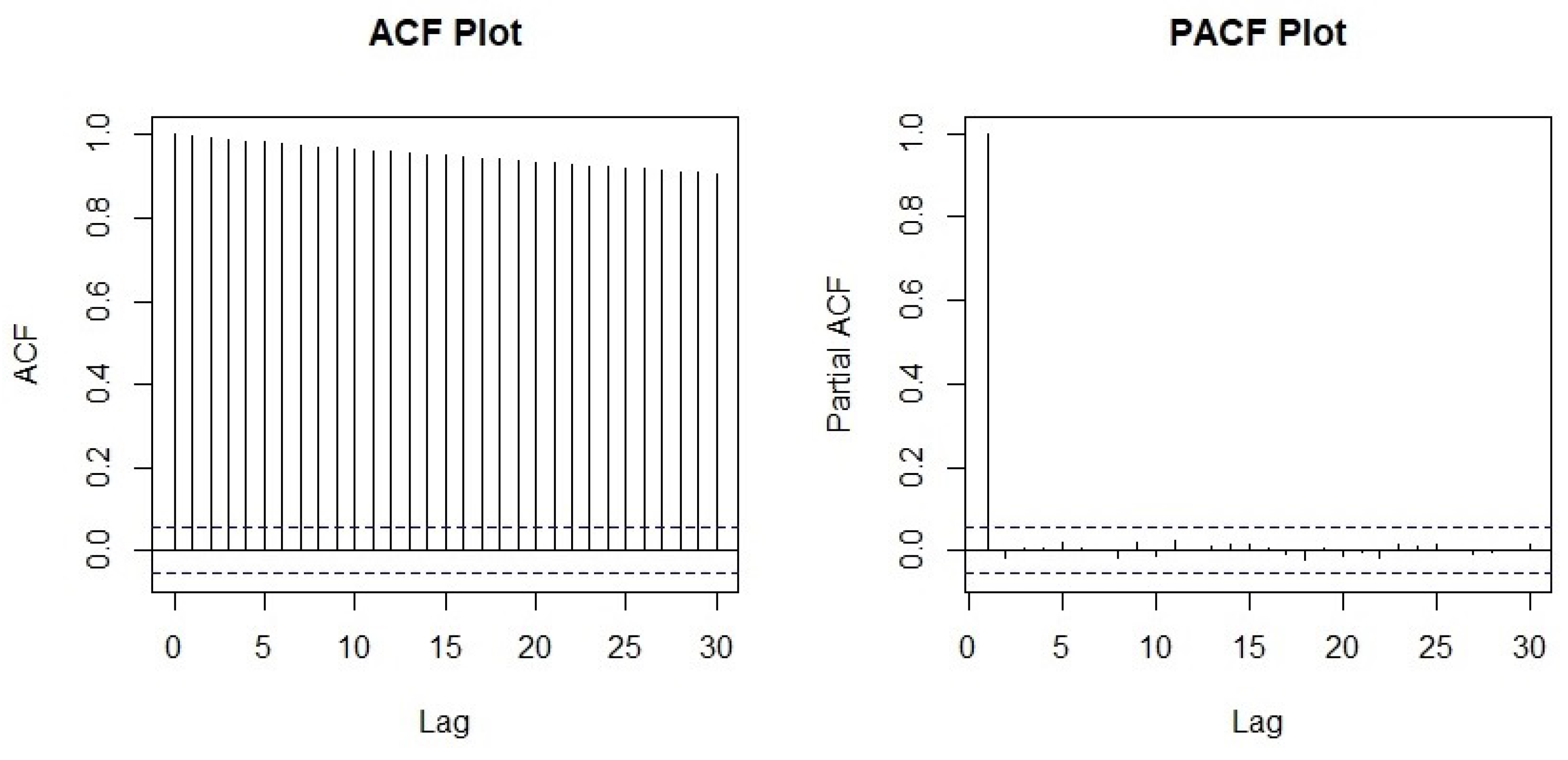
Jrfm 13 00181 g001
Figure 2. Sample autocorrelation plot.
Jrfm 13 00181 g002
Figure 3. Window plot of the second differenced log transformed stock price.
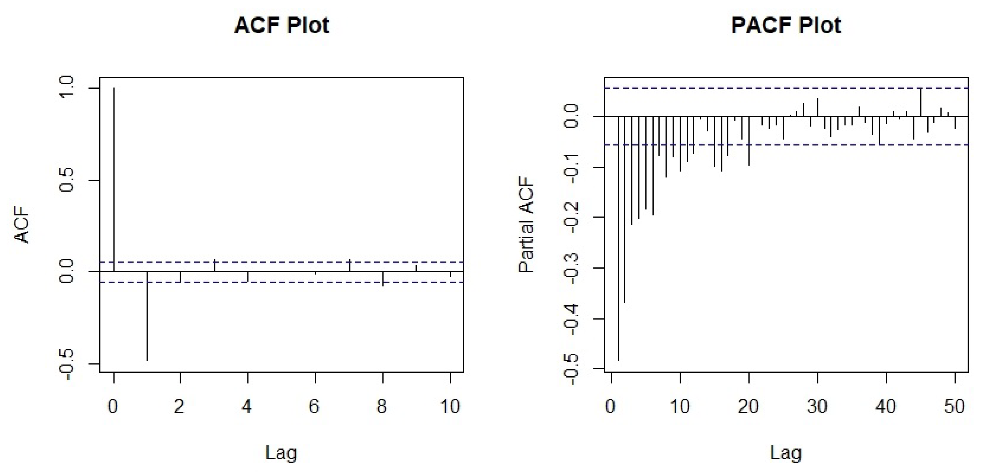
Jrfm 13 00181 g003
Figure 4. ACF and PACF of the second differenced log transformed stock price.
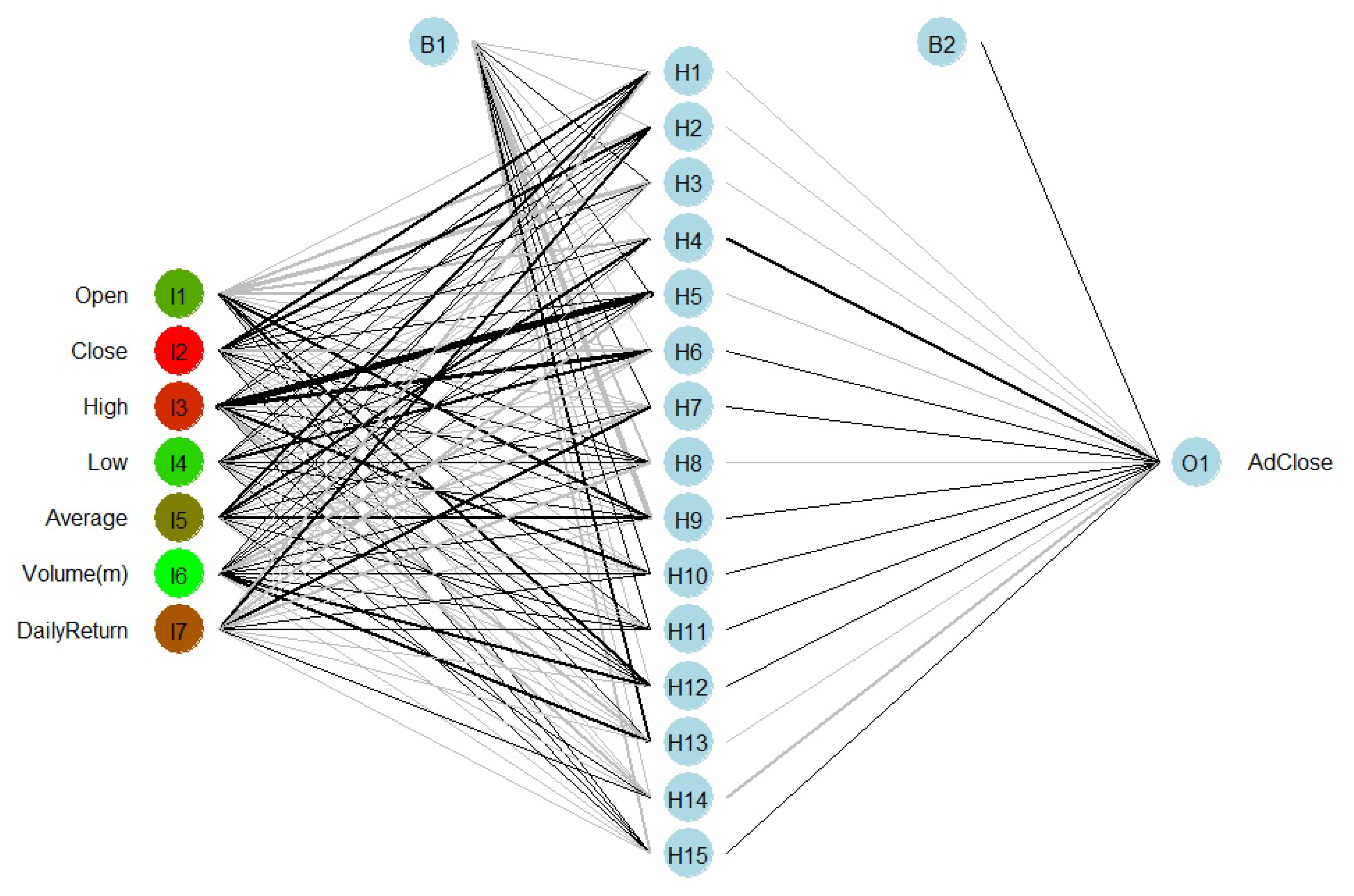
Jrfm 13 00181 g004
Figure 5. Artificial neural network architecture.
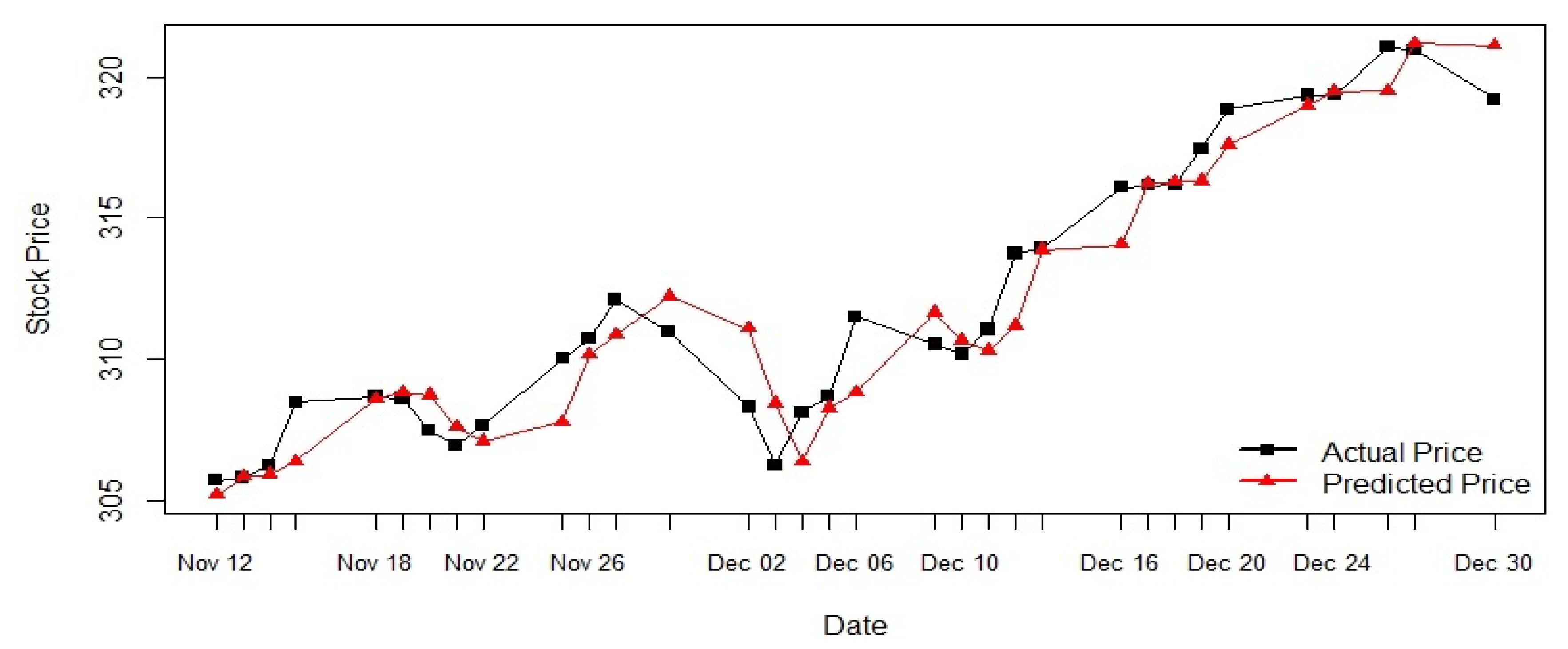
Jrfm 13 00181 g005
Figure 6. ARIMA (0,2,1) model prediction.
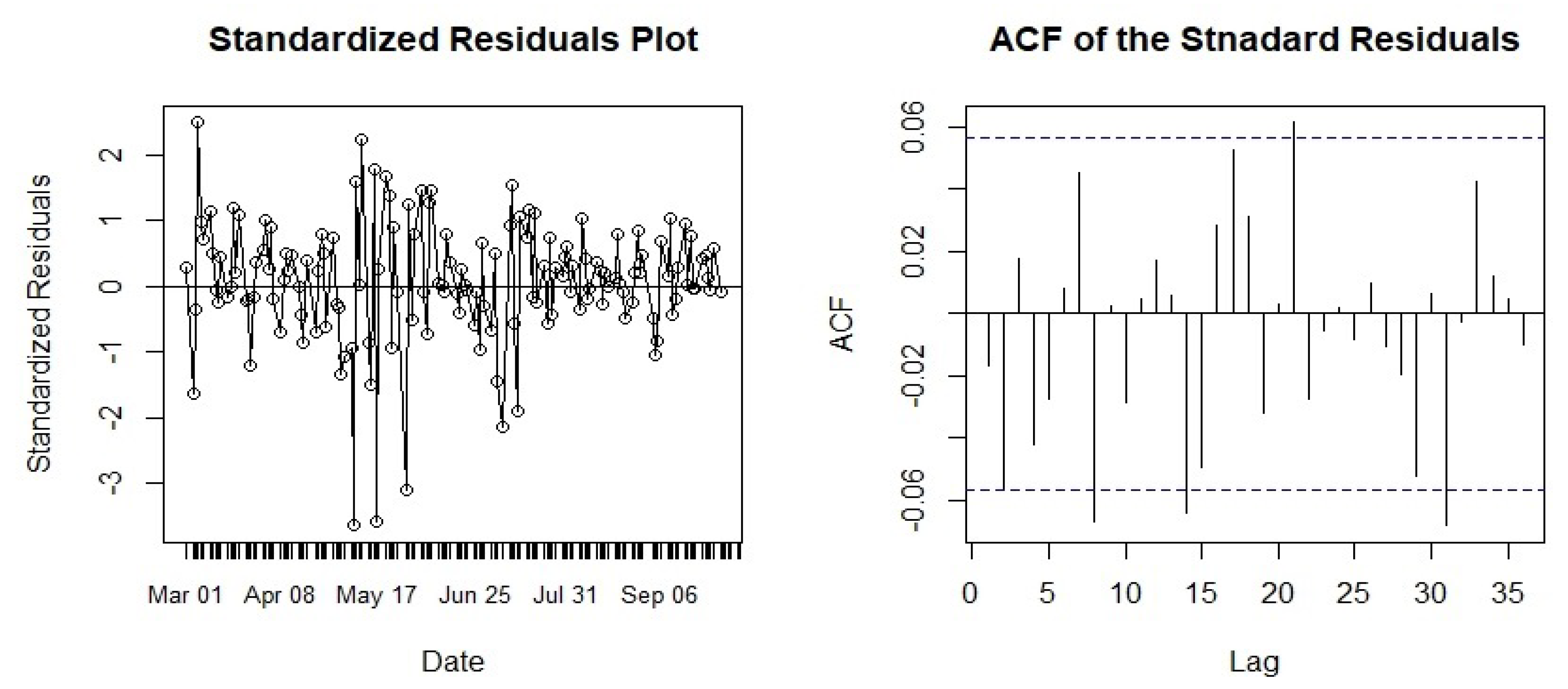
Jrfm 13 00181 g006
Figure 7. ARIMA(0,2,1) model residual analysis.
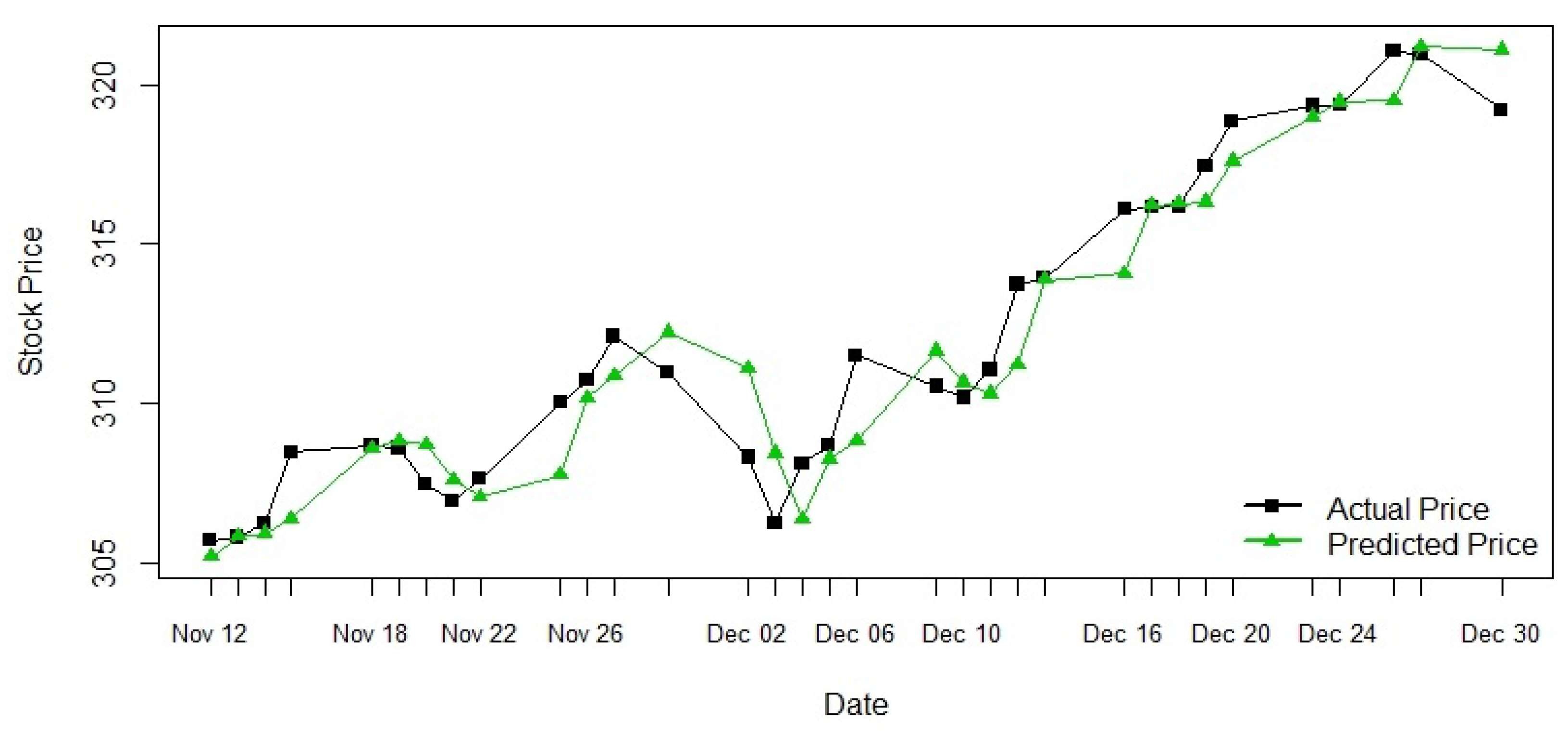
Jrfm 13 00181 g007
Figure 8. Stochastic model geometric Brownian motion prediction.
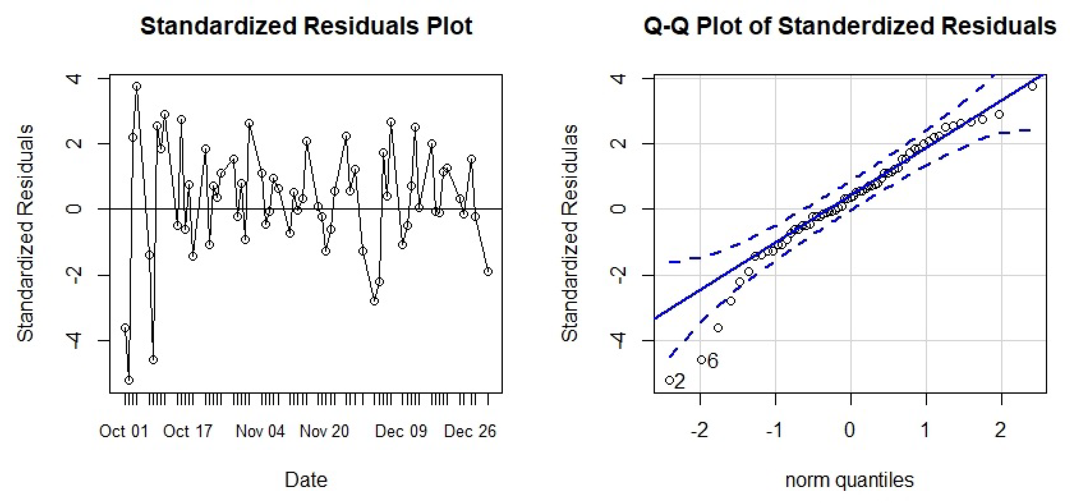
Jrfm 13 00181 g008
Figure 9. GBM model diagnostics.
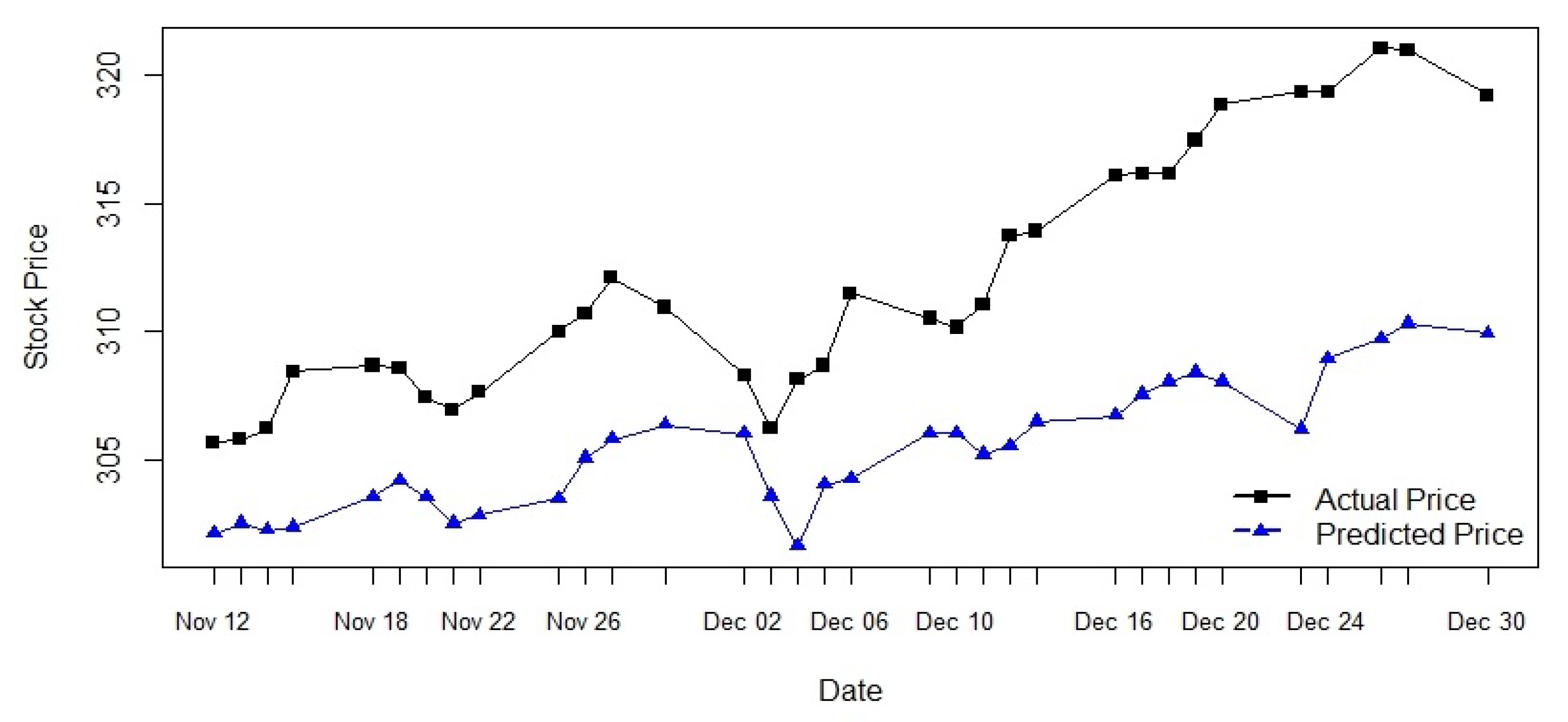
Jrfm 13 00181 g009
Figure 10. ANN(7-15-1) prediction.
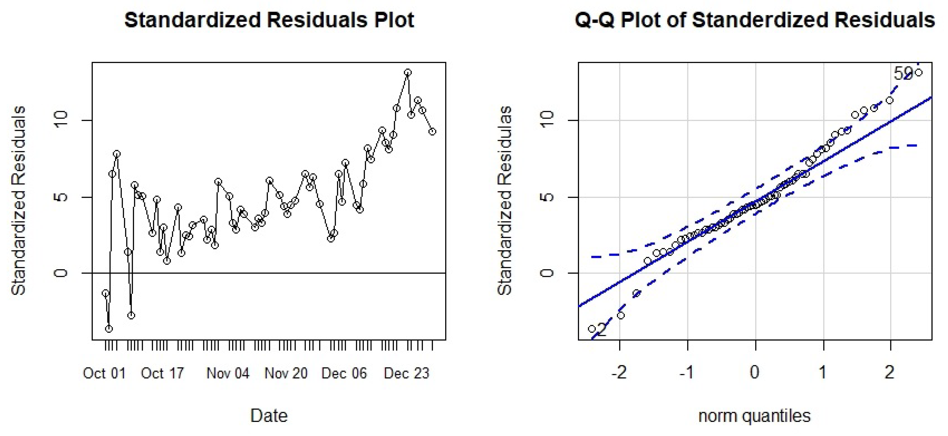
Jrfm 13 00181 g010
Figure 11. ANN(7-15-1) model diagnostics.
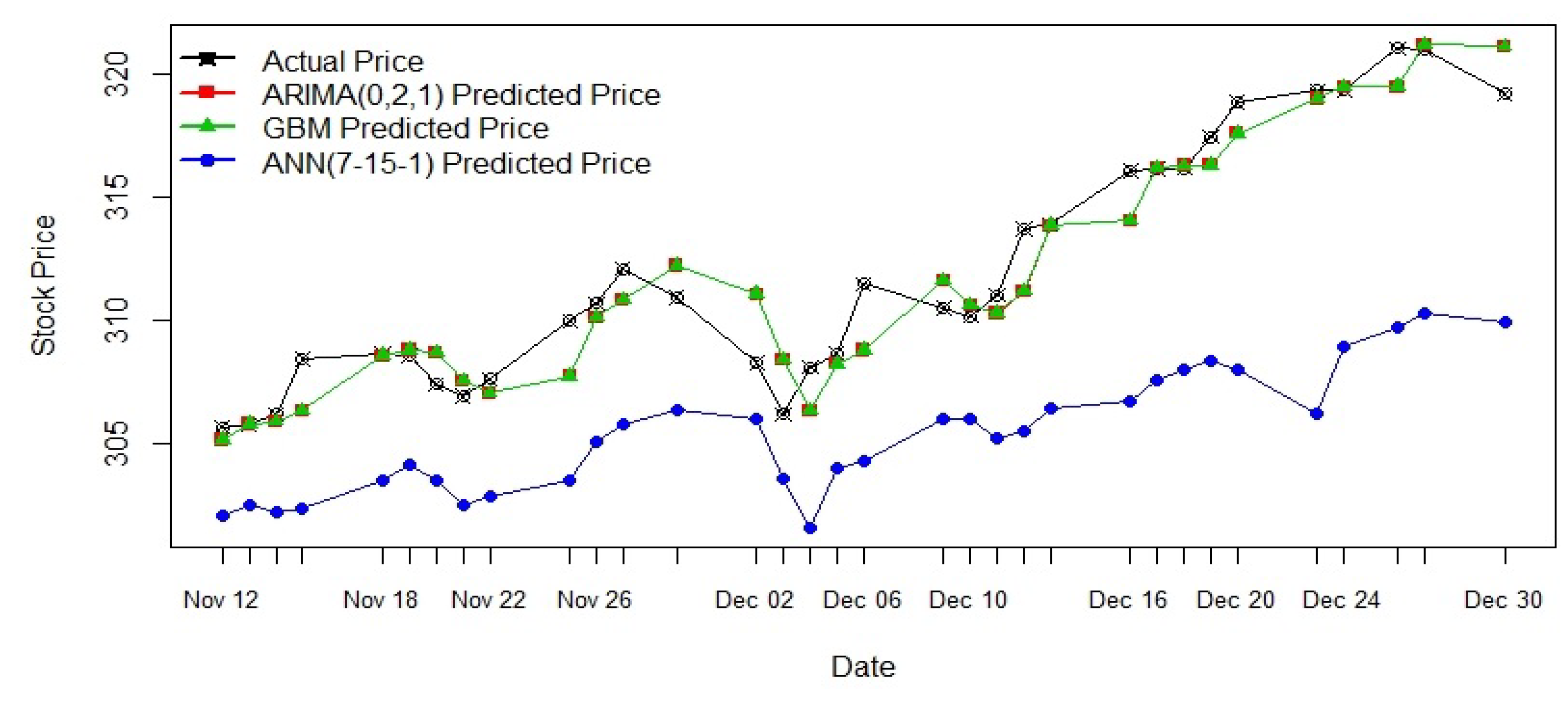
Jrfm 13 00181 g011
Figure 12. Prediction by all three models against the actual stock price.
Jrfm 13 00181 g012
Table 1. ARIMA (p,d,q) model comparison.
ModelAICBICAICc
ARIMA(0,2,0) 7144.11 7139.03 7144.11
ARIMA(0,2,1) 7981.48 7971.31 7981.47
ARIMA(0,2,2) 7979.84 7964.59 7979.82
ARIMA(0,2,3) 7981.77 7961.43 7981.73
ARIMA(0,2,4) 7980.02 7954.61 7979.97
ARIMA(1,2,0) 7455.29 7445.12 7455.28
ARIMA(1,2,1) 7979.81 7964.56 7979.79
ARIMA(1,2,2) 7982.16 7961.83 7982.13
ARIMA(1,2,3) 7983.04 7957.62 7982.98
ARIMA(1,2,4) 7981.53 7951.03 7981.45
ARIMA(2,2,0) 7631.73 7616.48 7631.71
ARIMA(2,2,1) 7981.50 7961.16 7981.46
ARIMA(2,2,2) 7982.88 7957.46 7982.83
ARIMA(2,2,3) 7982.62 7952.12 7982.55
ARIMA(2,2,4) 7979.91 7944.32 7979.81
ARIMA(3,2,0) 7692.63 7672.30 7692.60
ARIMA(3,2,1) 7979.84 7954.42 7979.79
ARIMA(3,2,2) 7981.50 7951.00 7981.43
ARIMA(3,2,3) 7977.84 7942.25 7977.74
ARIMA(3,2,4) 7978.07 7937.40 7977.95
ARIMA(4,2,0) 7738.80 7713.39 7738.75
ARIMA(4,2,1) 7980.13 7949.63 7980.06
ARIMA(4,2,2) 7978.69 7943.11 7978.60
ARIMA(4,2,3) 7978.28 7937.61 7978.15
ARIMA(4,2,4) 7984.84 7939.09 7984.69
Table 2. ARIMA(0,2,1) model summary.
ModelArima(x = tr.stock, order = c(0, 2, 1))
MA(1) Coefficient−1.00
Standard Error0.0027
Sigma-squared estimated as0.0000718
Log likelihood3992.74
AIC−7981.48
AICc−7981.47
BIC−7971.31
Training set error measuresMERMSEMAEMPEMAPEMASEACF1
0.000130.008460.005730.002200.105610.99516−0.01682
Table 3. Error measures for different network structures.
MODEL R 2 APEAAEARPERMSE
7-2-10.31370.02317.04350.11180.3344
7-3-10.41580.02116.4120.10180.319
7-4-10.04220.0288.51280.13510.3676
7-5-10.03680.02928.87960.14090.3754
7-6-10.37160.02156.54960.1040.3224
7-7-10.34310.02266.86870.1090.3302
7-8-10.39070.02196.67810.1060.3256
7-9-10.40360.02126.47130.10270.3205
7-10-10.41080.02146.52370.10360.3218
7-11-10.51550.01955.92840.09410.3068
7-12-10.53920.01875.68020.09020.3003
7-13-10.47770.01945.89450.09360.3059
7-14-10.46760.01965.97020.09480.3078
7-15-10.62160.01675.09280.08080.2843
7-16-10.57010.01825.53820.08790.2965
Table 4. Prediction by ARIMA(0,2,1) model.
DateActualPredictedError
11-12-2019305.69305.170.17
11-13-2019305.79305.810.01
11-14-2019306.23305.910.10
11-15-2019308.45306.350.68
11-18-2019308.68308.570.04
11-19-2019308.59308.800.07
11-20-2019307.44308.710.41
11-21-2019306.95307.560.20
11-22-2019307.63307.070.18
11-25-2019310.01307.750.73
11-26-2019310.72310.140.19
11-27-2019312.10310.850.40
11-29-2019310.94312.230.41
12-2-2019308.30311.070.90
12-3-2019306.23308.430.72
12-4-2019308.12306.360.57
12-5-2019308.68308.250.14
12-6-2019311.50308.810.86
12-9-2019310.52311.640.36
12-10-2019310.17310.650.15
12-11-2019311.05310.300.24
12-12-2019313.73311.180.81
12-13-2019313.92313.860.02
12-16-2019316.08314.050.64
12-17-2019316.15316.210.02
12-18-2019316.17316.290.04
12-19-2019317.46316.310.36
12-20-2019318.86317.600.40
12-23-2019319.34319.000.11
12-24-2019319.35319.480.04
12-26-2019321.05319.490.49
12-27-2019320.97321.200.07
12-30-2019319.20321.120.60
Table 5. Prediction error by ARIMA(0,2,1) model.
MODELAPEAAEARPERMSE
ARIMA(0,2,1)0.00441.36510.02170.1472
Table 6. Prediction by geometric Brownian motion.
DateActualPredictedError
11-12-2019305.69305.170.17
11-13-2019305.79305.810.01
11-14-2019306.23305.910.10
11-15-2019308.45306.350.68
11-18-2019308.68308.590.03
11-19-2019308.59308.800.07
11-20-2019307.44308.710.41
11-21-2019306.95307.580.21
11-22-2019307.63307.060.19
11-25-2019310.01307.740.73
11-26-2019310.72310.150.18
11-27-2019312.10310.860.40
11-29-2019310.94312.230.41
12-2-2019308.30311.090.90
12-3-2019306.23308.430.72
12-4-2019308.12306.360.57
12-5-2019308.68308.250.14
12-6-2019311.50308.820.86
12-9-2019310.52311.630.36
12-10-2019310.17310.640.15
12-11-2019311.05310.300.24
12-12-2019313.73311.210.80
12-13-2019313.92313.880.01
12-16-2019316.08314.060.64
12-17-2019316.15316.210.02
12-18-2019316.17316.270.03
12-19-2019317.46316.310.36
12-20-2019318.86317.590.40
12-23-2019319.34319.000.11
12-24-2019319.35319.470.04
12-26-2019321.05319.510.48
12-27-2019320.97321.200.07
12-30-2019319.20321.110.60
Table 7. Prediction error by geometric Brownian motion.
MODELAPEAAEARPERMSE
GBM0.00441.33410.02120.1455
Table 8. Prediction by ANN (7-15-1) model.
DateActualPredictedError
11-12-2019305.69302.131.17
11-13-2019305.79302.521.07
11-14-2019306.23302.261.30
11-15-2019308.45302.391.97
11-18-2019308.68303.561.66
11-19-2019308.59304.191.43
11-20-2019307.44303.541.27
11-21-2019306.95302.521.44
11-22-2019307.63302.861.55
11-25-2019310.72305.061.82
11-27-2019312.10305.812.02
11-29-2019310.94306.381.47
12-2-2019308.30306.020.74
12-3-2019306.23303.590.86
12-4-2019308.12301.632.11
12-5-2019308.68304.031.51
12-6-2019311.50304.282.32
12-9-2019310.52306.051.44
12-10-2019310.17306.071.33
12-11-2019311.05305.231.87
12-12-2019313.73305.552.61
12-13-2019313.92306.482.37
12-16-2019316.08306.732.96
12-17-2019316.15307.562.72
12-18-2019316.17308.052.57
12-19-2019317.46308.402.85
12-20-2019318.86308.043.39
12-23-2019319.34306.204.11
12-24-2019319.35308.943.26
12-26-2019321.05309.713.53
12-27-2019320.97310.313.32
12-30-2019319.20309.932.90
Table 9. Prediction error by ANN(7-5-1) model.
MODELAPEAAEARPERMSE
ANN(7-15-1)0.01675.092790.080840.28432
Table 10. Sample results from the models—ARIMA(0,2,1), G B M ( μ , σ 2 ) , and ANN(7-15-1).
DateActualARIMAGBMANN
11-12-2019305.69305.17305.17302.13
11-13-2019305.79305.81305.81302.52
11-14-2019306.23305.91305.91302.26
11-15-2019308.45306.35306.35302.39
11-18-2019308.68308.57308.59303.56
11-19-2019308.59308.80308.80304.19
11-20-2019307.44308.71308.71303.54
11-21-2019306.95307.56307.58302.52
11-22-2019307.63307.07307.06302.86
11-25-2019310.01307.75307.74303.50
11-26-2019310.72310.14310.15305.06
11-27-2019312.10310.85310.86305.81
11-29-2019310.94312.23312.23306.38
12-2-2019308.30311.07311.09306.02
12-3-2019306.23308.43308.43303.59
12-4-2019308.12306.36306.36301.63
12-5-2019308.68308.25308.25304.03
12-6-2019311.50308.81308.82304.28
12-9-2019310.52311.64311.63306.05
12-10-2019310.17310.65310.64306.04
12-11-2019311.05310.30310.30305.23
12-12-2019313.73311.18311.21305.55
12-13-2019313.92313.86313.88306.48
12-16-2019316.08314.05314.06306.73
12-17-2019316.15316.21316.21307.56
12-18-2019316.17316.29316.27308.05
12-19-2019317.46316.31316.31308.40
12-20-2019318.86317.60317.59308.04
12-23-2019319.34319.00319.00306.20
12-24-2019319.35319.48319.47308.94
12-26-2019321.05319.49319.51309.71
12-27-2019320.97321.20321.20310.31
12-30-2019319.20321.12321.11309.93
Table 11. Error measures comparison from the three models.
MODELAPEAAEARPERMSE
ARIMA(0,2,1)0.004381.334760.021190.14556
GBM0.004381.334260.021180.14553
ANN(7-15-1)0.016725.092790.080840.28432

