CVaR Regression Based on the Relation between CVaR and Mixed-Quantile Quadrangles

Abstract

A popular risk measure, conditional value-at-risk (CVaR), is called expected shortfall (ES) in financial applications. The research presented involved developing algorithms for the implementation of linear regression for estimating CVaR as a function of some factors. Such regression is called CVaR (superquantile) regression. The main statement of this paper is: CVaR linear regression can be reduced to minimizing the Rockafellar error function with linear programming. The theoretical basis for the analysis is established with the quadrangle theory of risk functions. We derived relationships between elements of CVaR quadrangle and mixed-quantile quadrangle for discrete distributions with equally probable atoms. The deviation in the CVaR quadrangle is an integral. We present two equivalent variants of discretization of this integral, which resulted in two sets of parameters for the mixed-quantile quadrangle. For the first set of parameters, the minimization of error from the CVaR quadrangle is equivalent to the minimization of the Rockafellar error from the mixed-quantile quadrangle. Alternatively, a two-stage procedure based on the decomposition theorem can be used for CVaR linear regression with both sets of parameters. This procedure is valid because the deviation in the mixed-quantile quadrangle (called mixed CVaR deviation) coincides with the deviation in the CVaR quadrangle for both sets of parameters. We illustrated theoretical results with a case study demonstrating the numerical efficiency of the suggested approach. The case study codes, data, and results are posted on the website. The case study was done with the Portfolio Safeguard (PSG) optimization package, which has precoded risk, deviation, and error functions for the considered quadrangles.

1. Introduction

We start the introduction with a quick outline of the main result of this paper. The conditional value-at-risk (CVaR) is a popular risk measure. It is called expected shortfall (ES) in financial applications and it is included in financial regulations. This paper provides algorithms for the estimation of CVaR with linear regression as a function of factors. This task is of critical importance in practical applications involving low probability events.

By definition, CVaR is an integral of the value-at-risk (VaR) in the tail of a distribution. VaR can be estimated with the quantile regression by minimizing the Koenker–Bassett error function. This paper shows that CVaR can be estimated by minimizing a mixture of the Koenker–Bassett errors with an additional constraint. This mixture is called the Rockafellar error and it has been earlier used for CVaR estimation without a rigorous mathematical justification. One more equivalent variant of CVaR regression can be done by minimizing a mixture of CVaR deviations for finding all coefficients, except the intercept. In this case, the intercept is calculated using an analytical expression, which is the CVaR of the optimal residual without an intercept. The new mathematical result links quantile and CVaR regressions and shows that convex and linear programming methods can be straightforwardly used for CVaR estimation. Mathematical justification of the results involves a risk quadrangle concept combining regret, error, risk, deviation, and statistic notions.

Quantiles evaluating different parts of a distribution of a random value are quite popular in various applications. In particular, quantiles are used to estimate tail of a distribution (e.g., 90%, 95%, and 99% quantiles). This paper is motivated by finance applications, where a quantile is called VaR. Risk measure VaR is included in finance regulations for the estimation of market risk. VaR has several attractive properties, such as the simplicity of calculation, stability of estimation, and availability of quantile regression, for the estimation of VaR as a function of explanatory factors. The quantile regression (see Koenker and Bassett (1978), Koenker (2005)) is an important factor supporting the popularity of VaR. For instance, a quantile regression was used by Adrian and Brunnermeier (2016) to estimate institution’s contribution to systemic risk.

However, VaR also has some undesirable properties:

• Lack of convexity: portfolio diversification may increase VaR.
• VaR is not sensitive to outcomes exceeding VaR, which allows for stretching of the distribution without an increasing of the risk measured by VaR.
• VaR has poor mathematical properties, such as discontinuity with respect to (w.r.t.) portfolio positions for discrete distributions based on historical data.

Shortcomings of VaR led financial regulators to use an alternative measure of risk, which is called conditional value-at-risk (CVaR) in this paper. This risk measure was introduced in Rockafellar and Uryasev (2000) and further studied in Rockafellar and Uryasev (2002) and many other papers. CVaR for continuous distributions equals the conditional expectation of losses exceeding VaR. An important mathematical fact is that CVaR is a coherent risk measure (see Acerbi and Tasche (2002), Rockafellar and Uryasev (2002)). Ziegel (2014) shows that CVaR is elicitable in a week sense. Fissler and Ziegel (2015) proved that (VaR, CVaR) is jointly elicitable, meaning elic(CVaR) ≤ 2, and more generally, that spectral risk measures have a low elicitation complexity. These results clarify the regression procedure of Rockafellar et al. (2014); their algorithm implicitly tracks the quantiles suggested by elicitation complexity.

Rockafellar and Uryasev (2000, 2002) have shown that CVaR of a convex function of variables is also a convex function. Due to this property, CVaR optimization problems can be reduced to convex and linear optimization problems.

This paper is based on risk quadrangle theory, which defines quadrangles (i.e., groups) of stochastic functionals Rockafellar and Uryasev (2013). Every quadrangle contains risk, deviation, error, and regret (negative utility). These elements of the quadrangle are linked by the statistic function.

The relation of quantile regression and CVaR optimization was explained using a quantile quadrangle (see Rockafellar and Uryasev (2013)). It was shown that the Koenker–Bassett error function and CVaR belong to the same quantile quadrangle. By minimizing the Koenker–Bassett error function with respect to one parameter, we obtain the CVaR deviation (which is the CVaR for the centered random value). The optimal value of the parameter, which is called statistic, equals VaR. Therefore, the linear regression with the Koenker–Bassett error estimates VaR as a function of factors. The fact that statistic equals VaR and is also used for building the optimization approach for CVaR (see Rockafellar and Uryasev (2000, 2002)).

Another important contribution that takes advantage of quadrangle theory is the regression decomposition theorem proved in Rockafellar et al. (2008). With this decomposition theorem, the regression problem is decomposed in two steps: (1) minimization of deviation from the corresponding quadrangle, and (2) calculation of the intercept by using statistic from this quadrangle. For instance, by applying the decomposition theorem to the quantile quadrangle, we can do quantile regression by minimizing CVaR deviation for finding all regression coefficients, except the intercept. Then, the intercept is calculated by using VaR statistic.

CVaR can be approximated using the weighted average of VaRs with different confidence levels, which is called the mixed VaR method. Rockafellar and Uryasev (2013) demonstrated that mixed VaR is a statistic in the mixed-quantile quadrangle. The error function, corresponding to this quadrangle (called the Rockafellar error) can be minimized for the estimation of the mixed VaR with linear regression. The Rockafellar error is a solution of a minimization problem with one linear constraint. Linear regression for estimating mixed VaR can be done by minimizing the Rockafellar error with convex and linear programming (Appendix A contains these formulations). Alternatively, this regression can be done in two steps with the decomposition theorem. The deviation in the mixed-quantile quadrangle is the mixed CVaR deviation, therefore all regression coefficients, except the intercept, can be found by minimizing this deviation. Further, the intercept can be found by using statistic, which is the mixed VaR.

Rockafellar et al. (2014) developed the CVaR quadrangle with the statistic equal to CVaR. Risk envelopes and identifiers for this quadrangle were calculated in Rockafellar and Royset (2018). This CVaR quadrangle is a theoretical basis for constructing the regression for estimating CVaR. Rockafellar et al. (2014) called the linear regression for estimation of CVaR using superquantile (CVaR) regression. The superquantile is an equivalent term for CVaR. Here we use the term “CVaR regression”. The CVaR regression plays a major role in various engineering areas, especially in financial applications. For instance, Huang and Uryasev (2018) used CVaR regression for the estimation of risk contributions of financial institutions and Beraldi et al. (2019) used CVaR for solving portfolio optimization problems with transaction costs.

This paper considers only discrete random values with a finite number of equally probable atoms. This special case is considered because it is needed for the implementation of the linear regression for the CVaR estimation. We have explained with an example how parameters of the optimization problems are calculated.

The equal probabilities property was used for calculating parameters of optimization problems. It is possible to calculate parameters with non-equal probabilities of atoms, but this is beyond the scope of the paper, which is focused on the linear regression.

We suggested two sets (Sets 1 and 2) of parameters for the mixed-quantile quadrangle. Set 1 corresponds to the two-step implementation of the CVaR regression in Rockafellar et al. (2014), and Set 2 is a new set of parameters. We proved that with Set 1, the statistic, risk, and deviation of the mixed-quantile and CVaR quadrangles coincide. Therefore, CVaR regression can be done by minimizing the Rockafellar error with convex and linear programming. For Set 2, the mixed-quantile and CVaR quadrangle share risk and deviation parameters. Also, the statistic of this mixed-quantile quadrangle (which may not be unique) includes statistic of the CVaR quadrangle. Therefore, minimizing the Rockafellar error correctly calculates all regression coefficients, but may provide an incorrect intercept. This is actually not a big concern because we know that the intercept is equal to the CVaR of an optimal residual without intercept.

Also, we demonstrated that the CVaR regression can be done in two steps with the decomposition theorem by using parameters from Sets 1 and 2 in the mixed-quantile deviation. A similar two-step procedure was used for CVaR regression in Rockafellar et al. (2014). Here we justify this two-step procedure through the equivalence of deviations in CVaR and mixed-quantile quadrangles with parameters from Sets 1 and 2.

This paper is organized as follows. Section 2 provides general results about quadrangles. In particular, we considered quantile, mixed-quantile, and CVaR quadrangles. Section 3 and Section 4 introduced and investigated the parameters from Sets 1 and 2, respectively. Section 5 provided optimization problem statements based on CVaR and mixed-quantile quadrangles and described the linear regression for CVaR estimation. Section 6 presented a case study and applied CVaR regression to the financial style classification problem. The case study is posted on the web with codes, data, and solutions. Appendix A provides convex and linear programming problems for minimization of the Rockafellar error; Appendix B provides Portfolio Safeguard (PSG) codes implementing regression optimization problems.

2. Quantile, Mixed-Quantile, and CVaR Quadrangles

Rockafellar and Uryasev (2013) developed a new paradigm called the risk quadrangle, which linked risk management, reliability, statistics, and stochastic optimization theories. The risk quadrangle methodology united risk functions for a random value $X$ in groups (quadrangles) consisting of five elements:

• Risk $ℛ\left(X\right)$, which provides a numerical surrogate for the overall hazard in $X$.
• Deviation $\mathcal{D}\left(X\right)$, which measures the “nonconstancy” in $X$ as its uncertainty.
• Error $ℰ\left(X\right)$, which measures the “nonzeroness” in $X$.
• Regret $\mathcal{V}\left(X\right)$, which measures the “regret” in facing the mix of outcomes of $X$.
• Statistic $\mathcal{S}\left(X\right)$ associated with $X$ through $ℰ$ and $\mathcal{V}$.

These elements of a risk quadrangle are related as follows:

$$\mathcal{V}\left(X\right)=ℰ\left(X\right)+E\left(X\right)$$

$$ℛ\left(X\right)=\mathcal{D}\left(X\right)+E\left(X\right)$$

$$ℛ\left(X\right)=\underset{C}{\min }\left\{C+\mathcal{V}\left(X-C\right)\right\}$$

$$\mathcal{D}\left(X\right)=\underset{C}{\min }\left\{ℰ\left(X-C\right)\right\}$$

$$\underset{C}{\mathrm{argmin}}\left\{C+\mathcal{V}\left(X-C\right)\right\}=\mathcal{S}\left(X\right)=\arg \underset{C}{\min }\left\{ℰ\left(X-C\right)\right\}$$

where $E\left(X\right)$ denotes the mean of $X$ and the statistic, $\mathcal{S}\left(X\right)$, can be a set, if the minimum is achieved for multiple points.

Further, we use the following notations. The cumulative distribution function is denoted by $F_X\left(x\right)=prob\left\{X\le x\right\}$. The positive and negative part of a number are denoted using:

$${\left[t\right]}^{+}=\{\begin{array}{c}t, \mathrm{for} t>0\\ 0, \mathrm{for} t\le 0\end{array} \mathrm{and} {\left[t\right]}^{-}=\{\begin{array}{c}-t, \mathrm{for} t<0\\ 0, \mathrm{for} t\ge 0\end{array}$$

The lower and upper VaR (quantile) are defined as follows:

lower VaR:

$$Va{R}_{\alpha }^{-}\left(X\right)=\{\begin{array}{c}sup\left\{x, F_X\left(x\right)<\alpha \right\}for 0<\alpha \le 1\\ inf\left\{x, F_X\left(x\right)\ge \alpha \right\} for \alpha =0\end{array}$$

upper VaR:

$$Va{R}_{\alpha }^{+}\left(X\right)=\{\begin{array}{c}inf\left\{x, F_X\left(x\right)>\alpha \right\} for 0\le \alpha <1\\ sup\left\{x, F_X\left(x\right)\le \alpha \right\} for \alpha =1\end{array}$$

VaR (quantile) is a set if the lower and upper quantiles do not coincide:

$$Va{R}_{\alpha }\left(X\right)=\left[Va{R}_{\alpha }^{-}\left(X\right),Va{R}_{\alpha }^{+}\left(X\right)\right]$$

otherwise VaR is a singleton $Va{R}_{\alpha }\left(X\right)=Va{R}_{\alpha }^{-}\left(X\right)=Va{R}_{\alpha }^{+}\left(X\right)$.

Conditional value-at-risk (CVaR) with the confidence level $\alpha \in \left(0,1\right)$ can be defined in many ways. We prefer the following constructive definition:

$$CVa{R}_{\alpha }\left(X\right)=\underset{C}{\min }\left\{C+\frac{1}{1-\alpha }E{[X-C]}^{+}\right\}$$

In financial applications, however, the most popular definition of CVaR is

$$CVa{R}_{\alpha }\left(X\right)=\frac{1}{1-\alpha }{\int }_{\alpha }^{1}Va{R}_{\beta }^{-}\left(X\right)d\beta .$$

For $\alpha =0,$ $CVa{R}_0\left(X\right)$ is defined as $CVa{R}_0\left(X\right)=\underset{\epsilon \to 0}{\lim } CVa{R}_{\epsilon }\left(X\right)=E\left(X\right)$.

For $\alpha =1, CVa{R}_1\left(X\right)$ is defined as $CVa{R}_1\left(X\right)=Va{R}_1^{-}\left(X\right)$ if a finite value of $Va{R}_1^{-}\left(X\right)$ exists.

Quadrangles are named after statistic functions. The most famous quadrangle is the quantile quadrangle (see Rockafellar and Uryasev (2013)), named after the VaR (quantile) statistic. This quadrangle establishes relations between the CVaR optimization technique described in Rockafellar and Uryasev (2000, 2002) and quantile regression (see Koenker and Bassett (1978), Koenker (2005)). In particular, it was shown that CVaR minimization and the quantile regression are similar procedures based on the VaR statistic in the regret and error representation of risk and deviation.

Here is the definition of the quantile quadrangle for $\alpha \in \left(0,1\right)$:

Quantile Quadrangle (Rockafellar and Uryasev (2013))

• Statistic: ${\mathcal{S}}_{\alpha }\left(X\right)=Va{R}_{\alpha }\left(X\right)$ = VaR (quantile) statistic.
• Risk: ${ℛ}_{\alpha }\left(X\right)=CVa{R}_{\alpha }\left(X\right)=\underset{C}{\min }\left\{C+{\mathcal{V}}_{\alpha }\left(X-C\right)\right\}=$ CVaR risk.
• Deviation: ${\mathcal{D}}_{\alpha }\left(X\right)=CVa{R}_{\alpha }\left(X\right)-E\left[X\right]=\underset{C}{\min }\left\{{ℰ}_{\alpha }\left(X-C\right)\right\}=$ CVaR deviation.
• Regret: ${\mathcal{V}}_{\alpha }\left(X\right)=\frac{1}{1-\alpha }E{\left[X\right]}^{+}=$ average absolute loss, scaled.
• Error: ${ℰ}_{\alpha }\left(X\right)=E\left[\frac{\alpha }{1-\alpha }{\left[X\right]}^{+}+{\left[X\right]}^{-}\right]= {\mathcal{V}}_{\alpha }\left(X\right)-E\left[X\right]=$ normalized Koenker–Bassett error.

The quantile quadrangle sets an example for development of more advances quadrangles. The following mixed-quantile quadrangle includes statistic, which is equal to the weighted average of VaRs (quantiles) with specified positive weights. Therefore, the error in this quadrangle can be used to build a regression for the weighted average of VaRs (quantiles). Since CVaR can be approximated by a weighted average of VaRs, the error function in this quadrangle can be used to build linear regression for the estimation of CVaR.

Mixed-Quantile Quadrangle (Rockafellar and Uryasev (2013)).

Confidence levels ${\alpha }_k\in \left(0,1\right), k=1,\dots ,r$, and weights ${\lambda }_k>0$, ${\sum }_{k=1}^r{\lambda }_k=1$. The error in this quadrangle is called the Rockafellar Error.

• Statistic: $\mathcal{S}\left(X\right)={\sum }_{k=1}^r{\lambda }_{k}Va{R}_{{\alpha }_k}\left(X\right)=$ mixed VaR (quantile).
• Risk: $ℛ\left(X\right)={\sum }_{k=1}^r{\lambda }_{k}CVa{R}_{{\alpha }_k}\left(X\right)=$ mixed CVaR.
• Deviation: $\mathcal{D}\left(X\right)={\sum }_{k=1}^r{\lambda }_{k}CVa{R}_{{\alpha }_k}\left(X-E\left[X\right]\right)=$ mixed CVaR deviation.
• Regret: $\mathcal{V}\left(X\right)=\underset{B_1,\dots ,B_r}{\min }\left\{{\sum }_{k=1}^r{\lambda }_k{\mathcal{V}}_{{\alpha }_k}\left(X-B_k\right)|{\sum }_{k=1}^r{\lambda }_k{B}_k=0\right\}=$ the minimal weighted average of regrets ${\mathcal{V}}_{{\alpha }_k}\left(X-B_k\right)=\frac{1}{1-{\alpha }_k}E{\left[X-B_k\right]}^{+}$ satisfying the linear constraint on $B_1,\dots ,B_r$.
• Error: $ℰ\left(X\right)=\underset{B_1,\dots ,B_r}{\min }\left\{{\sum }_{k=1}^r{\lambda }_k{ℰ}_{{\alpha }_k}\left(X-B_k\right)|{\sum }_{k=1}^r{\lambda }_k{B}_k=0\right\}=$ Rockafellar error $=$ the minimal weighted average of errors ${ℰ}_{{\alpha }_k}\left(X-B_k\right)=E\left[\frac{{\alpha }_k}{1-{\alpha }_k}{\left[X-B_k\right]}^{+}+{\left[X-B_k\right]}^{-}\right]$ satisfying the linear constraint on $B_1,\dots ,B_r.$

The following CVaR quadrangle can be considered as the limiting case of the mixed-quantile quadrangle when the number of terms in this quadrangle tends to infinity. The statistic in this quadrangle is CVaR; therefore, the error in this quadrangle can be used for the estimation of CVaR with linear regression.

CVaR Quadrangle (Rockafellar et al. (2014)) for $\alpha \in \left(0,1\right)$.

• Statistic: ${\overline{\mathcal{S}}}_{\alpha }\left(X\right)=CVa{R}_{\alpha }\left(X\right)$ = CVaR.
• Risk: ${\overline{ℛ}}_{\alpha }\left(X\right)=\frac{1}{1-\alpha }{\int }_{\alpha }^{1}CVa{R}_{\beta }\left(X\right)d\beta =$ CVaR2 risk.
• Deviation: ${\overline{\mathcal{D}}}_{\alpha }\left(X\right)={\overline{ℛ}}_{\alpha }\left(X\right)-E\left[X\right]=\frac{1}{1-\alpha }{\int }_{\alpha }^{1}CVa{R}_{\beta }\left(X\right)d\beta -E\left[X\right]=$ CVaR2 deviation.
• Regret: ${\overline{\mathcal{V}}}_{\alpha }\left(X\right)=\frac{1}{1-\alpha }{\int }_0^1{\left[CVa{R}_{\beta }\left(X\right)\right]}^{+}d\beta$ = CVaR2 regret.
• Error: ${\overline{ℰ}}_{\alpha }\left(X\right)={\overline{\mathcal{V}}}_{\alpha }\left(X\right)-E\left[X\right]$ = CVaR2 error.

The following section proves that for a discretely distributed random value with equally probable atoms, the CVaR quadrangle is “equivalent” to a mixed-quantile quadrangle with some parameters in the sense that statistic, risk, and deviation in these quadrangles coincide. This fact was proved for a set of random values with equal probabilities and variable locations of atoms.

The set of parameters considered in the following section is used in two-step CVaR regression in Rockafellar et al. (2014).

3. Set 1 of Parameters for Mixed-Quantile Quadrangle

Set 1 of parameters for the mixed-quantile quadrangle for a discrete uniformly distributed random value $X$ consists of confidence levels ${\alpha }_k\in \left(0,1\right),k=1,\dots ,r$ and weights ${\lambda }_k>0$ such that ${\sum }_{k=1}^r{\lambda }_k=1$. Parameter $r$ depends only on the number of atoms in $X$ and the confidence level $\alpha$ of the CVaR quadrangle. We proved that statistic, risk, and deviation of the mixed-quantile quadrangle with the Set 1 of parameters coincide with the statistic, risk, and deviation of the CVaR quadrangle.

Let $X$ be a discrete random value with support $x^i$ and $\mathrm{Prob}\left(X=x^i\right)=1/\nu$ for $i=1,2,\dots ,\nu$, where $\nu$ is the number of atoms. Denote $x^{max}=\underset{i=1,\dots ,\nu }{\max }{x}^i$. For this random value, $CVa{R}_1\left(X\right)=Va{R}_1^{-}\left(X\right)=x^{max}$.

Set 1 of parameters:

• partition of the interval $\left[\alpha ,1\right]$: ${\beta }_{{\nu }_{\alpha }-1}=\alpha$, and ${\beta }_i=i\delta$, for $i={\nu }_{\alpha }, {\nu }_{\alpha }+1,\dots ,\nu$, where $\delta =1/\nu$, ${\nu }_{\alpha }=\lfloor \nu \alpha \rfloor +1$, with $\lfloor z\rfloor$ being the largest integer less than or equal to $z$; ${\delta }_{\alpha }={\beta }_{{\nu }_{\alpha }}-\alpha$.
• weights: $p_{{\nu }_{\alpha }}=\frac{{\delta }_{\alpha }}{1-\alpha }, p_i=\frac{\delta }{1-\alpha }, i={\nu }_{\alpha }+1,\dots ,\nu$.
• confidence levels: ${\gamma }_i=1-\frac{{\beta }_i-{\beta }_{i-1}}{\ln \left(\frac{1-{\beta }_{i-1}}{1-{\beta }_i}\right)},i= {\nu }_{\alpha },\dots ,\nu -1$; ${\gamma }_{\nu }=1$.

Lemma 1.

Let$X$be a discrete random value with$\nu$equally probable atoms. Then, statistic, risk, and deviation of the CVaR quadrangle for$X$are given by the following expressions with parameters specified by Set 1:

1. 

CVaR statistic:

$${\overline{\mathcal{S}}}_{\alpha }\left(X\right)=CVa{R}_{\alpha }\left(X\right)={\sum }_{i={\nu }_{\alpha }}^{\nu }{p}_{i}Va{R}_{{\gamma }_i}\left(X\right)$$

(1)

2. 

CVaR2 risk:

$${\overline{ℛ}}_{\alpha }\left(X\right)=\frac{1}{1-\alpha }{\int }_{\alpha }^{1}CVa{R}_{\beta }\left(X\right)d\beta ={\sum }_{i={\nu }_{\alpha }}^{\nu }{p}_{i}CVa{R}_{{\gamma }_i}\left(X\right)$$

(2)

3. 

CVaR2 deviation:

$${\overline{\mathcal{D}}}_{\alpha }\left(X\right)=\frac{1}{1-\alpha }{\int }_{\alpha }^{1}CVa{R}_{\beta }\left(X\right)d\beta -E\left[X\right]={\sum }_{i={\nu }_{\alpha }}^{\nu }{p}_{i}CVa{R}_{{\gamma }_i}\left(X\right)-E\left[X\right]$$

(3)

Proof. 

Appendix C contains proof of the lemma. □

Note. 

Expression (1) is valid for arbitrary ${\gamma }_i\in \left({\beta }_{i-1},{\beta }_i\right)$, $i={\nu }_{\alpha },\dots ,\nu$. Equations (2) and (3) are valid for arbitrary ${\gamma }_{\nu }\in [{\beta }_{\nu -1},1].$

We want to emphasize that the statement of Lemma 1 is valid for any discrete random value with equally probable atoms. The statement does not depend upon atom locations.

Corollary 1.

For the random value$X$defined in Lemma 1, statistic, risk, and deviation of the CVaR quadrangle coincide with statistic, risk, and deviation of the mixed-quantile quadrangle with$r=\nu -{\nu }_{\alpha }+1$,${\lambda }_k=p_{{\nu }_{\alpha }-1+k}$,${\alpha }_k={\gamma }_{{\nu }_{\alpha }-1+k}$,$k=1,\dots ,r$.

Proof. 

Right hand sides in Equations (1)–(3) define statistic, risk, and deviation of the mixed-quantile quadrangle because $p_i>0, i={\nu }_{\alpha },\dots ,\nu$, ${\sum }_{i={\nu }_{\alpha }}^{\nu }{p}_i$ = 1 and $Va{R}_{{\gamma }_i}\left(X\right), i={\nu }_{\alpha },\dots ,\nu$, are singletons. □

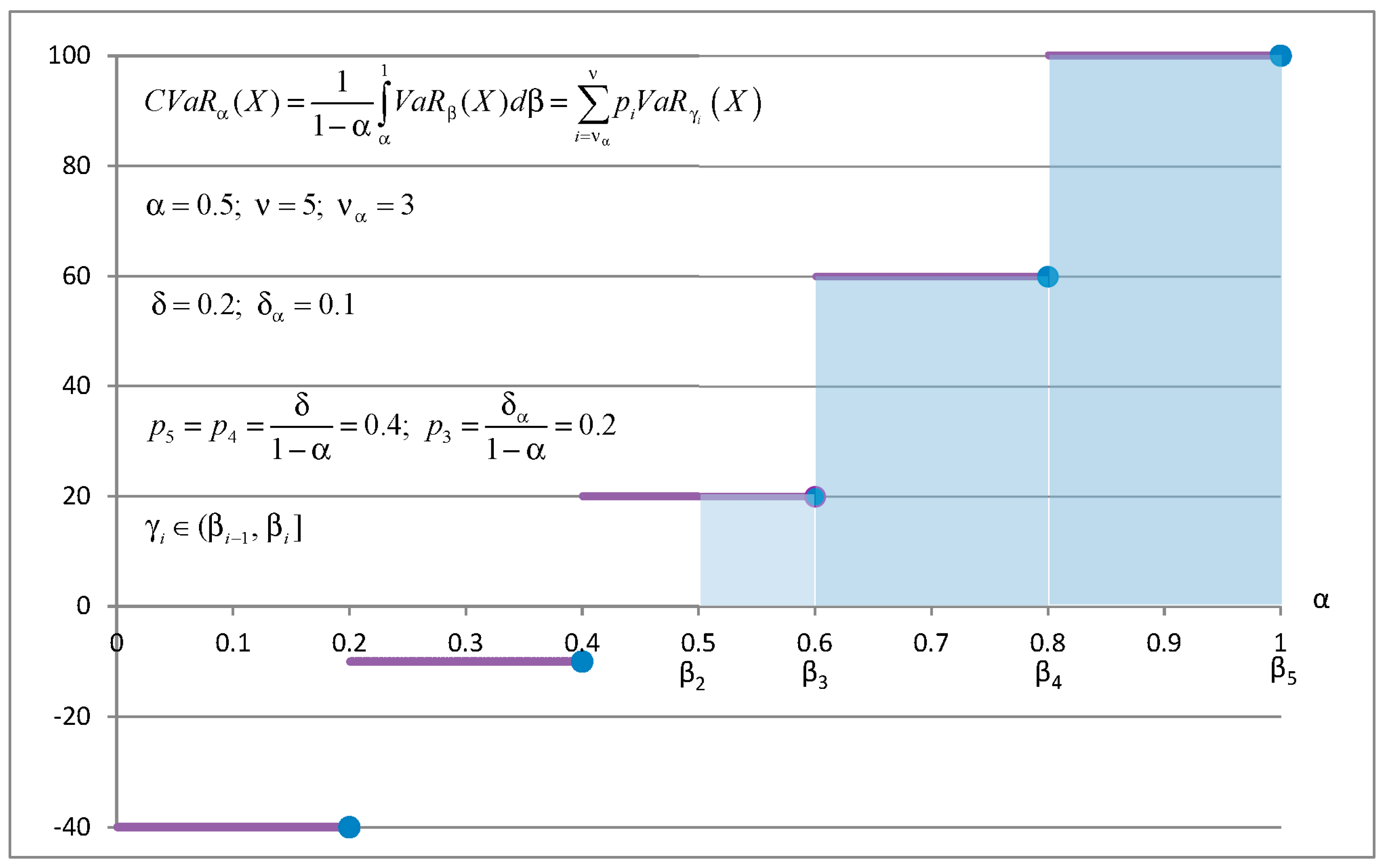
Example 1.

Let$X$be a discrete random value with five atoms (−40; −10; 20; 60 100) and equal probabilities = 0.2.

Figure 1 explains how to calculate statistic in the CVaR quadrangle and mixed-quantile quadrangle with Set 1 of parameters for $\alpha =0.5$. Bold lines show $Va{R}_{\alpha }^{-}\left(X\right)$ as a function of $\alpha .$ $CVa{R}_{0.5}\left(X\right)$ equals the dark area under the $Va{R}_{\alpha }\left(X\right)$ divided by $1-\alpha$. CVaR can be calculated as integral of $Va{R}_{\alpha }\left(X\right)$ or as the sum of areas of rectangles. 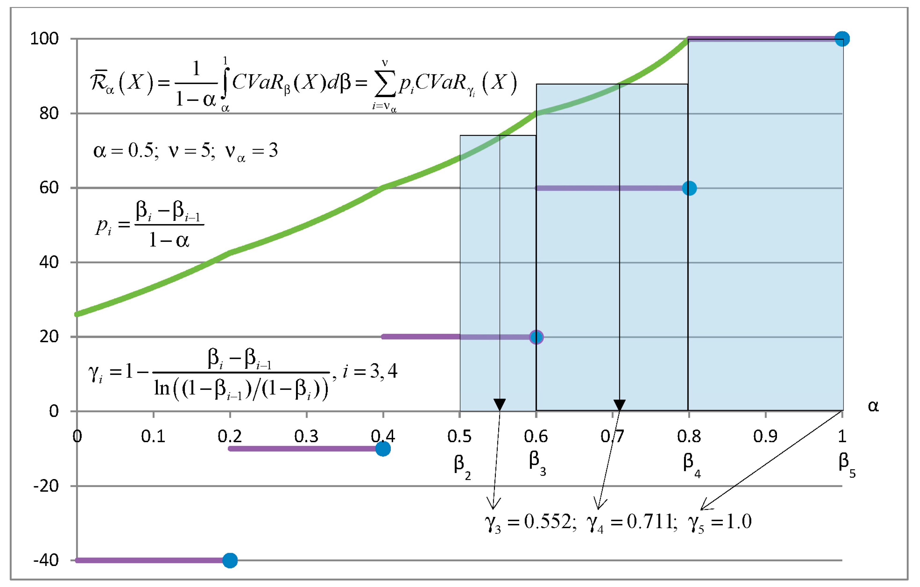Figure 2 explains how to calculate risk in the CVaR quadrangle and mixed-quantile quadrangle with Set 1 of parameters for $\alpha =0.5$. The bold continuous curve shows $CVa{R}_{\alpha }\left(X\right)$ as a function of $\alpha$. Risk ${\overline{ℛ}}_{0.5}\left(X\right)$ is equal to the area under the CVaR curve divided by $1-\alpha$. This area can be calculated as the integral of CVaR or as the sum of areas of rectangles. The area of every rectangle is equal to the area under CVaR in the appropriate range of $\alpha$. The equality of areas defines values of ${\gamma }_i$. Parameters $p_i, {\gamma }_i$ do not depend on the values of atoms.

4. Set 2 of Parameters for the Mixed-Quantile Quadrangle

This section gives an alternative expression for the risk ${\overline{ℛ}}_{\alpha }\left(X\right)$ and deviation ${\overline{\mathcal{D}}}_{\alpha }\left(X\right)$ in the CVaR quadrangle for a discrete uniformly distributed random variable. This expression is based on the following Set 2 of parameters. This set of parameters has the same number of parameters as Set 1 but different values of weights and confidence levels. Similar to Section 3, let $X$ be a discrete random value with support, $x^i$, $i=1,2,\dots ,\nu$, and $\mathrm{Prob}\left(X=x^i\right)=1/\nu$ for $i=1,2,\dots ,\nu$. Denote $x^{max}=\underset{ i=1,\dots ,\nu }{ \max }{x}^i$. For this random value $CVa{R}_1\left(X\right)=Va{R}_1^{-}\left(X\right)=x^{max}$.

Set 2 of parameters:

• partition of the interval $\left[{\beta }_{{\nu }_{\alpha }-1},1\right]$: $\delta =1/\nu$, ${\beta }_i=i\delta$, for $i={\nu }_{\alpha }-1, {\nu }_{\alpha },\dots ,\nu$, where ${\nu }_{\alpha }=\lfloor \nu \alpha \rfloor +1$, with $\lfloor z\rfloor$ being the largest integer less than or equal to $z$; ${\delta }_{\alpha }={\beta }_{{\nu }_{\alpha }}-\alpha$.
• confidence levels: ${\beta }_i$, $i={\nu }_{\alpha }-1, {\nu }_{\alpha },\dots ,\nu$.
• weights:
  $q_{\nu }=0$;
  $q_{\nu -1}=\frac{\delta }{1-\alpha }\times \left[2\ln \left(2\right)\right]\approx \frac{\delta }{1-\alpha }\times 1.386294361$, $(\mathrm{if} \nu -1>{\nu }_{\alpha })$
  $q_{\nu -2}=\frac{\delta }{1-\alpha }\times 2\left[3\ln \left(\frac{3}{2}\right)+\ln \left(\frac{1}{2}\right)\right]\approx \frac{\delta }{1-\alpha }\times 1.046496288$, $(\mathrm{if} \nu -2>{\nu }_{\alpha })$
  $q_{\nu -j}=\frac{\delta }{1-\alpha }\times j\left[\left(j+1\right)\ln \left(\frac{j+1}{j}\right)+\left(j-1\right)\ln \left(\frac{j-1}{j}\right)\right]$, $(\mathrm{if} j>2,\nu -j>{\nu }_{\alpha })$
  $q_{{\nu }_{\alpha }} =\frac{\delta }{1-\alpha }\times j\left[\delta -{\delta }_{\alpha }+\left(j+1\right)\ln \left(\frac{1-\alpha }{\delta j}\right)+\left(j-1\right)\ln \left(\frac{j-1}{j}\right)\right]$, ($\mathrm{if} {\nu }_{\alpha }<\nu -1, j=\nu -{\nu }_{\alpha })$
  $q_{{\nu }_{\alpha }-1}=\frac{\delta }{1-\alpha }\times j\left[{\delta }_{\alpha }+\left(j-1\right)\ln \left(\frac{\delta \left(j-1\right)}{1-\alpha }\right)\right]$, $(\mathrm{if} {\nu }_{\alpha }-1<\nu -1, j=\nu -{\nu }_{\alpha }+1$)
  if ${\nu }_{\alpha }=\nu -1$, then $q_{{\nu }_{\alpha }}=\frac{\delta }{1-\alpha }\times 2\left[1+\ln \left(\frac{1-\alpha }{\delta }\right)\right]-1$, $q_{{\nu }_{\alpha }-1}=\frac{\delta }{1-\alpha }\times 2\left[\ln \left(\frac{\delta }{1-\alpha }\right)-1\right]+2$
  if ${\nu }_{\alpha }=\nu$, then $q_{{\nu }_{\alpha }-1}=1.$

Lemma 2.

Let$X$be a discrete random value with$\nu$equally probable atoms. Then, risk and deviation of the CVaR quadrangle for$X$are given by the following expressions with parameters from Set 2.

1. 

CVaR2 Risk:

$${\overline{ℛ}}_{\alpha }\left(X\right)=\frac{1}{1-\alpha }{\int }_{\alpha }^{1}CVa{R}_{\beta }\left(X\right)d\beta ={\sum }_{i={\nu }_{\alpha }-1}^{\nu -1}{q}_{i}CVa{R}_{{\beta }_i}\left(X\right)$$

(4)

2. 

CVaR2 Deviation:

$${\overline{\mathcal{D}}}_{\alpha }\left(X\right)=\frac{1}{1-\alpha }{\int }_{\alpha }^{1}CVa{R}_{\beta }\left(X\right)d\beta -E\left[X\right]={\sum }_{i={\nu }_{\alpha }-1}^{\nu -1}{q}_{i}CVa{R}_{{\beta }_i}\left(X\right)-E\left[X\right]$$

(5)

Proof. 

Appendix D contains proof of the lemma. □

Note. 

Equations (4) and (5) are valid if $CVa{R}_{{\beta }_{\nu -1}}$ is replaced by $CVa{R}_{\gamma }$ with an arbitrary $\gamma \in [{\beta }_{\nu -1},1].$

Corollary 2.

For the random value$X$defined in Lemma 2, risk and deviation of the CVaR quadrangle coincide with risk and deviation of the mixed-quantile quadrangle with$r=\nu -{\nu }_{\alpha }+1$,${\lambda }_k=q_{{\nu }_{\alpha }-2+k}$,${\alpha }_k={\beta }_{{\nu }_{\alpha }-2+k}$,$k=1,\dots ,r$.

Proof. 

Right hand sides in Equations (4) and (5) define risk and deviation of the mixed-quantile quadrangle because $q_i>0, i={\nu }_{\alpha }-1,\dots ,\nu -1$, and ${\sum }_{i={\nu }_{\alpha }-1}^{\nu -1}{q}_i=1$. □

Lemma 3.

Let$X$be a discrete random value with equally probable atoms$x^i$,$i=1,2,\dots ,\nu$,$Prob\left(X=x^i\right)=1/\nu$. Then, statistic of the mixed-quantile quadrangle defined by the Set 2 of parameters is a range containing statistic of the CVaR quadrangle.

Proof. 

Appendix E contains proof of the lemma. □

5. On the Estimation of CVaR with Mixed-Quantile Linear Regression

This section formulates regression problems using the CVaR quadrangle and mixed-quantile quadrangle. For discrete final distributions with equally probable atoms, we prove some equivalence statements for the CVaR and mixed-quantile quadrangles. Further, we demonstrate how to estimate CVaR by using the linear regression with error and deviation from the mixed-quantile quadrangle.

We want to estimate variable $V$ using a linear function $f\left(\mathit{Y}\right)=C_0+{\mathit{C}}^T\mathit{Y}$ of the explanatory factors $\mathit{Y}=$ $\left(Y_1,\dots ,Y_n\right).$ Let $\widetilde{ℰ}$ be an error from some quadrangle (further we consider, mixed-quantile and CVaR quadrangles), and $\tilde{\mathcal{D}}$ and $\tilde{\mathcal{S}}$ be a deviation and a statistic, respectively, corresponding to this quadrangle. Below we consider optimization statements for solving regression problems.

General Optimization Problem 1

Minimize error $\widetilde{ℰ}$ and find optimal $C_0^{*}, {\mathit{C}}^{*}$

$$\underset{C_0\in ℝ, \mathit{C}\in {ℝ}^m}{min}\widetilde{ℰ} \left(Z\left(C_0,\mathit{C}\right)\right)$$

where Z$\left(C_0,\mathit{C}\right)=V-C_0-{\mathit{C}}^T\mathit{Y}$.

General Optimization Problem 2

• Step 1. Find an optimal vector${\mathit{C}}^{*}$by minimizing deviation:

  $$\underset{\mathit{C}\in {ℝ}^m}{min }\tilde{\mathcal{D}}\left(Z_0\left(\mathit{C}\right)\right)$$

  where$Z_0\left(\mathit{C}\right)=V-{\mathit{C}}^T\mathit{Y}$.
• Step 2. Assign$C_0^{*}$:

  $$C_0^{*}\in \tilde{\mathcal{S}}\left(Z_0\left({\mathit{C}}^{*}\right)\right)$$

Error $\widetilde{ℰ} \left(X\right)$ is called nondegenerate if:

$$\underset{X:EX=D}{ inf}\widetilde{ℰ} \left(X\right)>0 \mathrm{for} \mathrm{constants} D\ne 0.$$

Rockafellar et al. (2008), p. 722, proved the following decomposition theorem.

Theorem 1.

(Error-Shaping Decomposition of Regression). Let$\widetilde{ℰ}$be a nondegenerate error and$\tilde{\mathcal{D}}\underset{C}{=\mathit{min}}\left\{\widetilde{ℰ}\left(X-C\right)\right\}$be the corresponding deviation, and let$\tilde{\mathcal{S}}$be the associated statistic. Point ($C_0^{*}$,${\mathit{C}}^{*}$) is a solution of the General Optimization Problem 1 if and only if${\mathit{C}}^{*}$is a solution of the General Optimization Problem 2, Step 1 and$C_0^{*}\in \tilde{\mathcal{S}}\left(Z_0\left({\mathit{C}}^{*}\right)\right)$with Step 2.

According to the decomposition theorem, when $\widetilde{ℰ}$, $\tilde{\mathcal{D}}$, and $\tilde{\mathcal{S}}$ are elements of the CVaR quadrangle, the following Optimization Problems 1 and 2 are equivalent.

Optimization Problem 1

Minimize error from the CVaR quadrangle:

$$\underset{C_0\in ℝ, \mathit{C}\in {ℝ}^m}{ min}{\overline{ℰ}}_{\alpha }\left(Z\left(C_0,\mathit{C}\right)\right)$$

where Z$\left(C_0,\mathit{C}\right)=V-C_0-{\mathit{C}}^T\mathit{Y}$.

Optimization Problem 2

• Step 1. Find an optimal vector${\mathit{C}}^{*}$by minimizing deviation from the CVaR quadrangle:

  $$\underset{\mathit{C}\in {ℝ}^m}{min} {\overline{\mathcal{D}}}_{\alpha }\left(Z_0\left(\mathit{C}\right)\right)$$

  where$Z_0\left(\mathit{C}\right)=V-{\mathit{C}}^T\mathit{Y}$.
• Step 2. Calculate:

  $$C_0^{*}=CVa{R}_{\alpha }\left(Z_0\left({\mathit{C}}^{*}\right)\right)$$

In Optimization Problem 2 in Step 2 the statistic equals $\overline{S}\left(Z_0\left({\mathit{C}}^{*}\right)\right)=CVa{R}_{\alpha }\left(Z_0\left({\mathit{C}}^{*}\right)\right)$, which is the specification of the inclusion operation in the Optimization Problem General 2 in Step 2.

Optimization Problem 2 is used in Rockafellar et al. (2014) for the construction of the linear regression algorithms for estimating CVaR.

According to the decomposition theorem, when $\widetilde{ℰ}$, $\tilde{\mathcal{D}}$, and $\tilde{\mathcal{S}}$ are elements of a mixed-quantile quadrangle, the following Optimization Problems 3 and 4 are equivalent.

Optimization Problem 3

Minimize error from the mixed-quantile quadrangle:

$$\underset{C_0\in ℝ, \mathit{C}\in {ℝ}^m}{min}ℰ\left(Z\left(C_0,\mathit{C}\right)\right)$$

Optimization Problem 4

• Step 1. Find an optimal vector${\mathit{C}}^{*}$by minimizing deviation from the mixed-quantile quadrangle:

  $$\underset{\mathit{C}\in {ℝ}^m}{min } \mathcal{D}\left(Z_0\left(\mathit{C}\right)\right)$$
• Step 2. Assign:

  $$C_0^{*}\in \mathcal{S}\left(Z_0\left({\mathit{C}}^{*}\right)\right)$$

Corollaries 1 and 2 can be used for constructing the linear regression for estimating CVaR. Let $\mathit{Y}$ be a random vector of factors for estimating the random value $V$. We consider that the linear regression function $f\left(\mathit{Y}\right)=C_0+{\mathit{C}}^T\mathit{Y}$ approximates CVaR of $V$, where $C_0\in ℝ, \mathit{C}\in {ℝ}^m$ are variables in the linear regression. The residual is denoted by $Z\left(C_0,\mathit{C}\right)=V-\left(C_0+{\mathit{C}}^T\mathit{Y}\right)$ and $Z_0\left(\mathit{C}\right)=V-{\mathit{C}}^T\mathit{Y}$.

Further we provide a lemma about linear regression problems based on Corollary 1 with the Set 1 of parameters. The main statement here is that the Optimization Problems 3 and 4 for the mixed-quantile quadrangle can be used to solve linear regression problems for estimating CVaR. This is the case because CVaR and mixed-quantile quadrangles have the same Statistic and Deviation.

Lemma 4.

Let the residual random value$Z\left(C_0,\mathit{C}\right)=V-\left(C_0+{\mathit{C}}^T\mathit{Y}\right)$be discretely distributed with$\nu$equally probable atoms. Let us consider the CVaR quadrangle with error${\overline{ℰ}}_{\alpha }\left(Z\left(C_0,\mathit{C}\right)\right)$, deviation${\overline{\mathcal{D}}}_{\alpha }\left(Z_0\left(\mathit{C}\right)\right)$, and statistic${\overline{S}}_{\alpha }\left(Z_0\left({\mathit{C}}^{*}\right)\right)$. Let us also consider the mixed-quantile quadrangle with the error$ℰ\left(Z\left(C_0,\mathit{C}\right)\right)$, deviation$\mathcal{D}\left(Z_0\left(\mathit{C}\right)\right)$, and statistic$\mathcal{S}\left(Z_0\left({\mathit{C}}^{*}\right)\right)$with parameters defined by Set 1 and$r=\nu -{\nu }_{\alpha }+1$,${\lambda }_k=p_{{\nu }_{\alpha }-1+k}$,${\alpha }_k={\gamma }_{{\nu }_{\alpha }-1+k}$,$k=1,\dots ,r$. Then, the Optimization Problems 1–4 are equivalent, i.e., the sets of optimal vectors of these optimization problems coincide. Moreover, let$\left(C_0^{*},{\mathit{C}}^{*}\right)$be a solution vector of the equivalent Optimization Problems 1–4. Then:

$$C_0^{*}=CVa{R}_{\alpha }\left(Z_0\left({\mathit{C}}^{*}\right)\right)$$

$${\overline{ℰ}}_{\alpha }\left(C_0^{*},{\mathit{C}}^{*}\right)= ℰ\left(C_0^{*},{\mathit{C}}^{*}\right)= \mathcal{D}\left(Z_0\left({\mathit{C}}^{*}\right)\right)={\overline{\mathcal{D}}}_{\alpha }\left(Z_0\left({\mathit{C}}^{*}\right)\right)$$

Proof. 

This lemma is a direct corollary of the decomposition Theorem 1 and Corollary 1 of Lemma 1. Indeed, Corollary 1 implies that the Optimization Problems 2 and 4 are equivalent. Further, the decomposition theorem implies that Optimization Problems 1 and 2 and the Optimization Problems 3 and 4 are equivalent. □

Further we provide a lemma about linear regression problems based on Corollary 2 with the Set 2 of parameters. The main statement is that the Optimization Problem 4, Step 1 for the Mixed-Quantile Quadrangle can be used to solve linear regression problem for estimating CVaR. This is the case because CVaR and Mixed-Quantile Quadrangles have the same Deviation. After obtaining vector of coefficients ${\mathit{C}}^{*}$, intercept is calculated, $C_0^{*}=CVa{R}_{\alpha }\left(Z_0\left({\mathit{C}}^{*}\right)\right)$.

Lemma 5.

Let the residual random value$Z\left(C_0,\mathit{C}\right)=V-\left(C_0+{\mathit{C}}^T\mathit{Y}\right)$be discretely distributed with$\nu$equally probable atoms. Let the mixed-quantile quadrangle with deviation$\mathcal{D}\left(Z_0\left(\mathit{C}\right)\right)$be defined by parameters of Set 2 and$r=\nu -{\nu }_{\alpha }+1$,${\lambda }_k=q_{{\nu }_{\alpha }-2+k}$,${\alpha }_k={\beta }_{{\nu }_{\alpha }-2+k}$,$k=1,\dots ,r$. Then,$\left(C_0^{*},{\mathit{C}}^{*}\right)$is a solution of Optimization Problem 1, if and only if,$\left(C_0^{*},{\mathit{C}}^{*}\right)$is a solution of the following two-step procedure:

• Step 1. Find an optimal vector${\mathit{C}}^{*}$by minimizing deviation from the mixed-quantile quadrangle:

  $$\underset{\mathit{C}\in {ℝ}^m}{min } \mathcal{D}\left(Z_0\left(\mathit{C}\right)\right)$$
• Step 2. Calculate$C_0^{*}=CVa{R}_{\alpha }\left(Z_0\left({\mathit{C}}^{*}\right)\right)$.

Proof. 

This lemma is a direct corollary of the decomposition Theorem 1 and Corollary 2 or Lemma 2. Indeed, the Corollary 2 implies that the Optimization Problems 2 and 4 are equivalent. Further, since deviations of the CVaR and mixed-quantile quadrangles coincide, we can use Step 1 to calculate optimal coefficients ${\mathit{C}}^{*}$. Further, the intercept is calculated with $C_0^{*}=CVa{R}_{\alpha }\left(Z_0\left({\mathit{C}}^{*}\right)\right)$ because CVaR is the statistic in the CVaR quadrangle. □

For the Set 2 of parameters, the deviations in the CVaR and mixed-quintile quadrangles coincide. The two-step procedure in Optimization Problem 4 can be used to solve linear regression problems with Set 2 parameters for the mixed-quantile deviation. Also, the minimization of the Rockafellar error with the Set 2 of parameters may result in a correct ${\mathit{C}}^{*}$. The statistic of CVaR belongs to the statistic of the mixed-quantile quadrangle. Therefore, the optimization of the Rockafellar error with the Set 2 of parameters may lead to a wrong value of intercept $C_0^{*}$. This potential incorrectness can be fixed by assigning $C_0^{*}=CVa{R}_{\alpha }\left(Z_0\left({\mathit{C}}^{*}\right)\right)$.

6. Case Study: Estimation of CVaR with Linear Regression and Style Classification of Funds

The case study described in this section is posted online (see Case Study (2016)). The codes and data are available for downloading and verification. Every optimization problem is presented in three formats: Text, MATLAB, and R. Calculations were done with a PC with a 3.14 GHz processor.

We have applied CVaR regression to the return-based style classification of a mutual fund. We regress a fund return by several indices as explanatory factors. The estimated coefficients represent the fund’s style with respect to each of the indices.

A similar problem with a standard regression based on the mean squared error was considered by Carhart (1997) and Sharpe (1992). They estimated the conditional expectation of a fund return distribution (under the condition that a realization of explanatory factors is observed). Basset and Chen (2001) extended this approach and conducted the style analyses of quantiles of the return distribution. This extension is based on the quantile regression suggested by Koenker and Bassett (1978). The Case Study (2014), “Style Classification with Quantile Regression” implemented this approach and applied quantile regression to the return-based style classification of a mutual fund.

For the numerical implementation of CVaR linear regression, we used the Portfolio Safeguard (2018) package. Portfolio Safeguard (PSG) can solve nonlinear and mixed-integer nonlinear optimization problems. A special feature of PSG is that it includes precoded nonlinear functions: CVaR2 error (cvar2_err) and CVaR2 deviation (cvar2_dev) from the CVaR quadrangle, Rockafellar error (ro_err) from the mixed-quantile quadrangle, and CVaR deviation (cvar_dev) from the quantile quadrangle.

We implemented the following equivalent variants of CVaR regression:

• Minimization of the CVaR2 error (PSG function cvar2_err).
• Two-step procedure with CVaR2 deviation (PSG function cvar2_dev).
• Minimization of the Rockafellar error (PSG function ro_err) with the Set 1 of parameters.
• The two-step procedure using mixed CVaR deviation with the Set 1 and Set 2 of parameters. This is calculated as a weighted sum of CVaR deviations (PSG function cvar_dev) from the quantile quadrangle.

PSG automatically converts the analytic problem formulations to the mathematical programming codes and solves them. We included in Appendix A convex and linear programming problems for the minimization of the Rockafellar error with the Set 1 of parameters. These formulations are provided for verification purposes. They can be implemented with standard commercial software. For instance, the linear programming formulation can be implemented with the Gurobi optimization package. If Gurobi is installed in the computer, PSG can use Gurobi code as a subsolver. With the CARGRB solver in PSG, by setting the linearize option to 1, it is possible to solve the linear programming problem with Gurobi. However, this conversion will deteriorate the performance, compared to the default PSG solver VAN. For small problems it will not be noticeable. However, for problems with a large number of scenarios (e.g., with 10⁸ observations), the standard PSG solver VAN will dramatically outperform the Gurobi linear programming implementation. In this case, Gurobi may not even start on a small PC because of a shortage of memory. Nevertheless, if the number of observations is small (e.g., 10³) and the number of factors is very large (e.g., 10⁷), it is recommended that the linear programming formulation is used.

We regressed the CVaR of the return distribution of the Fidelity Magellan Fund on the explanatory variables: Russell 1000 Growth Index (RLG), Russell 1000 Value Index (RLV), Russell Value Index (RUJ), and Russell 2000 Growth Index (RUO). The dataset includes 1264 historical daily returns of the Magellan Fund and the indices, which were downloaded from the Yahoo Finance website. The data (design matrix for the regression) is posted on the Case Study (2016) website.

The CVaR regression was done with the confidence levels $\alpha =$ 0.75 and $\alpha =$ 0.9. Calculation results are in

Table 1. Optimization outputs: estimating CVaR with the linear regression, $\alpha =$ 0.75.

Optimization Problem #	Set #	Objective	RLG	RLV	RUJ	RUO	Intercept	Solving Time (s)
1	N/A	0.01248	0.486	0.581	−0.0753	−6.22 × 10−3	6.98 × 10−3	0.02
2	N/A	0.01248	0.486	0.582	−0.0753	−6.22 × 10−3	6.98 × 10−3	0.02
3	Set 1	0.01247	0.486	0.582	−0.0753	−6.22 × 10−3	6.96 × 10−3	0.03
4	Set 1	0.01251	0.486	0.582	−0.0752	−6.22 × 10−3	6.98 × 10−3	0.11
4	Set 2	0.01248	0.486	0.582	−0.0753	−6.23 × 10−3	6.98 × 10−3	0.03

and

Table 2. Optimization outputs: estimating CVaR with the linear regression, $\alpha =$ 0.9.

Optimization Problem #	Set #	Objective	RLG	RLV	RUJ	RUO	Intercept	Solving Time (s)
1	N/A	0.016656	0.472	0.606	−0.078	−7.052 × 10−3	1.05 × 10−2	0.02
2	N/A	0.016656	0.472	0.606	−0.078	−7.052 × 10−3	1.05 × 10−2	0.02
3	Set 1	0.016656	0.472	0.606	−0.078	−7.052 × 10−3	1.05 × 10−2	0.02
4	Set 1	0.016656	0.472	0.606	−0.078	−7.052 × 10−3	1.05 × 10−2	0.11
4	Set 2	0.016656	0.472	0.606	−0.078	−7.052 × 10−3	1.05 × 10−2	0.04

, respectively. Here is the description of the columns of the tables:

• Optimization Problem #: Optimization Problem number, as denoted in Section 5; also it is the problem number in the case study posted online, see, Case Study (2016).
• Set #: Set of parameters for the mixed-quantile quadrangle.
• Objective: Optimal value of the objective function.
• RLG: coefficient for the Russell Value Index.
• RLV: coefficient for the Russell 1000 Value Index.
• RUJ: coefficient for the Russell Value Index.
• RUO: coefficient for the Russell 2000 Growth Index.
• Intercept: regression intercept.
• Solving Time: solver optimization time.

Table 1 and Table 2 show calculation results for the considered equivalent problems. We observe that regression coefficients coincide for all problems in Table 1 and Table 2. This confirms the correctness of theoretical results and the numerical implementation. Also, we want to point out that the regression coefficients are quite similar for $\alpha =$ 0.75 (Table 1) and $\alpha =$ 0.9 (Table 2).

The calculation time in majority of cases was around 0.02–0.04 s, except for the case with the mixed CVaR deviation for Set 1, which took 0.11 s. The PSG calculation times were quite low because the solver “knows” analytical expressions for the functions and can take advantage of this knowledge.

7. Conclusions

The quadrangle risk theory Rockafellar and Uryasev (2013) and the decomposition theorem Rockafellar et al. (2008) provided a framework for building a regression with relevant deviations. Solution of a regression problem is split in two steps: (1) minimization of deviation from the corresponding quadrangle, and (2) determining of intercept by using statistic from this quadrangle. For CVaR regression, Rockafellar et al. (2014) reduced the optimization problem at Step 1 to a high-dimension linear programming problem. We suggested two sets of parameters for the mixed-quantile quadrangle and investigated its relationship with the CVaR quadrangle. The Set 1 of parameters corresponds to CVaR regression in Rockafellar et al. (2014), where the Set 2 is a new set of parameters.

For the Set 1 of parameters, the minimization of error from CVaR Quadrangle was reduced to the minimization of the Rockafellar error from the mixed-quantile quadrangle. For both sets of parameters, the minimization of deviation in CVaR quadrangle is equivalent to the minimization of deviation in mixed-quantile quadrangle.

We presented optimization problem statements for CVaR regression problems using CVaR and mixed-quantile quadrangles. Linear regression problem for estimating CVaR were efficiently implemented in Portfolio Safeguard (2018) with convex and linear programming. We have done a case study for the return-based style classification of a mutual fund with CVaR regression. We regressed the fund return by several indices as explanatory factors. Numerical results validating the theoretical statements are placed to the web (see Case Study (2016)).