
Modeling Production-Living-Ecological Space for Chengdu, China: An Analytical Framework Based on Machine Learning with Automatic Parameterization of Environmental Elements

 and
and
Abstract
:1. Introduction
- This study realizes the dynamic and automatic identification of the key elements that affect the evolution of the PLES under multi-object scenarios, which advances the toolbox for land use simulation methods and provide a framework for other case studies.
- Our investigation focuses on a typical southwestern Chinese city, which is one of the core cities in large urban agglomeration in southwest China. The evidence from this new case study could help mitigate the imbalance issue between research on the eastern and western regions in China and offer insights for other developing countries.
- We applied a finer land use classification data, combined with machine learning algorithms and multi-objective scenario simulation to study PLES, which offers new perspectives of land-use simulation and analytics for policy and decision makers.
2. A Brief Literature Review
2.1. The Core of PLES: Automatic Parameterization of Environmental Element
2.2. Empirical Research on PLES
2.3. PLES Combined with Multi-Categorical Land Use Data and Machine Learning Algorithms
3. Data Collection
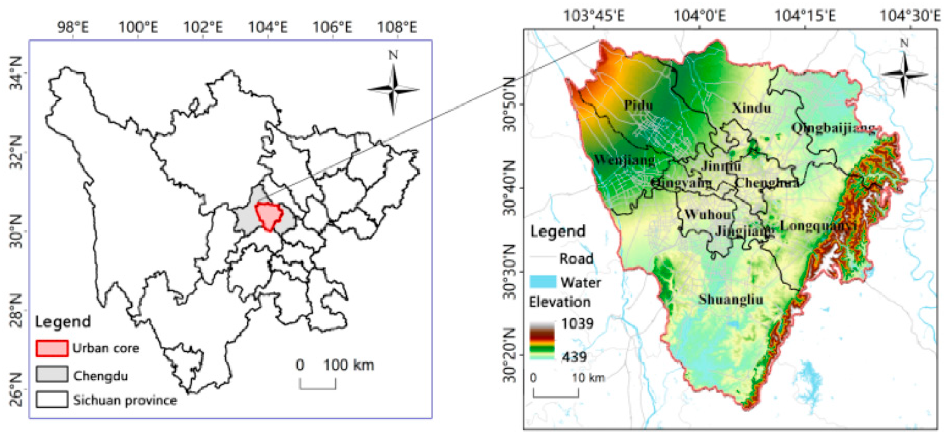
3.1. Study Area
3.2. Data Source
- geological conditions, including geological disaster points and digital elevation model (DEM).
- ecological environment conditions, including ecological environment quality, biodiversity, net primary production (NPP), farmland production potential, soil erosion, and normalized difference vegetation index (NDVI);
- climatic conditions, including annual average temperature, annual precipitation;
- economic conditions, including point of interest (POI) and night lights as the driving factors for the simulation model inputs.
3.3. Data Treatment and Pre-Processing
4. Methods
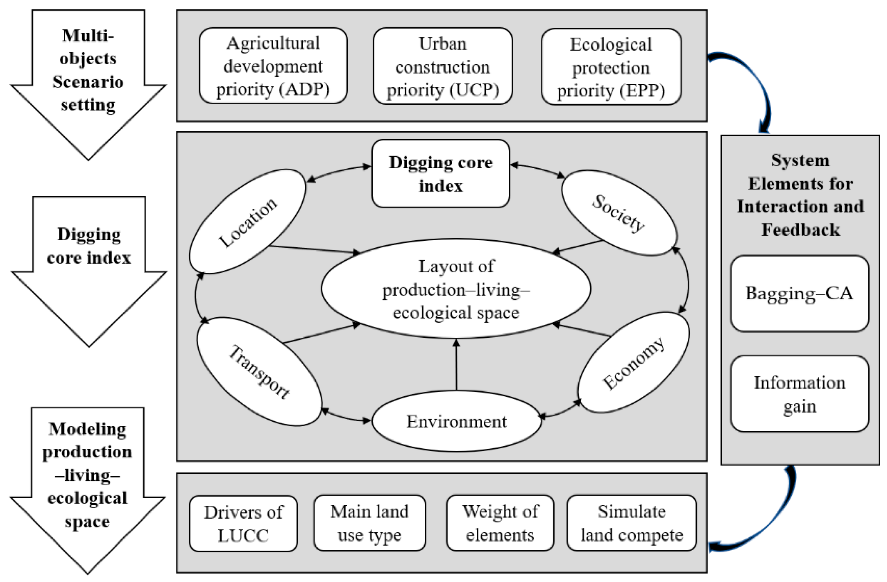
4.1. Analytical Framework
4.2. Simulation Scenario Design
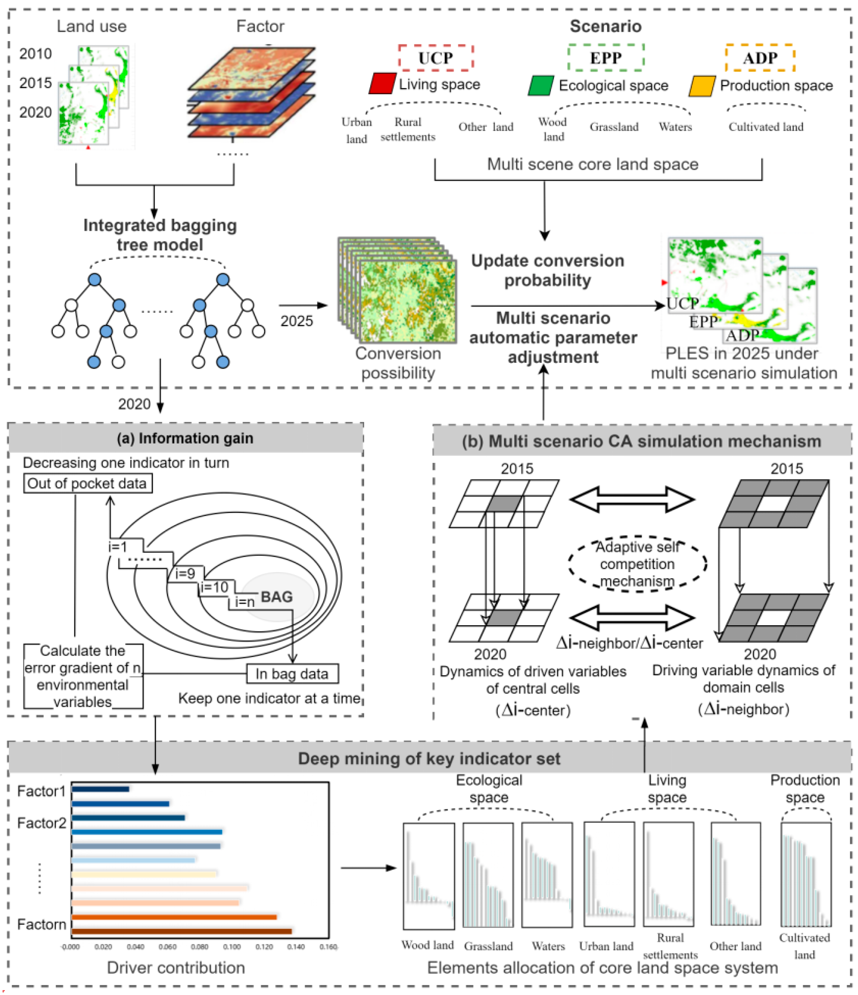
4.3. Bagging Algorithm
- First, the information entropy of N-dimensional features in the initial system was calculated.
- Next, we removed the features sequentially and calculated the information entropy carried by the new system after removing each feature. Then, by calculating the difference between the information entropy carried by the initial system and that by the new system, the information gain of each feature on the whole data set was evaluated, and the estimation error of the out-of-pocket data was obtained.
- The information entropy carried by the new system after only one feature was kept in turn was calculated. The difference between the information entropy carried by the new system and the average information entropy carried by each feature of the initial system was calculated, and the estimation error of the data in the bag was obtained.
- The estimation errors of in-bag and out-of-bag data were averaged to obtain the degree of contribution of each feature to the whole data set, which was the weight of the corresponding index.
4.4. Spatio-Temporal Cellular Automata Model
5. Results
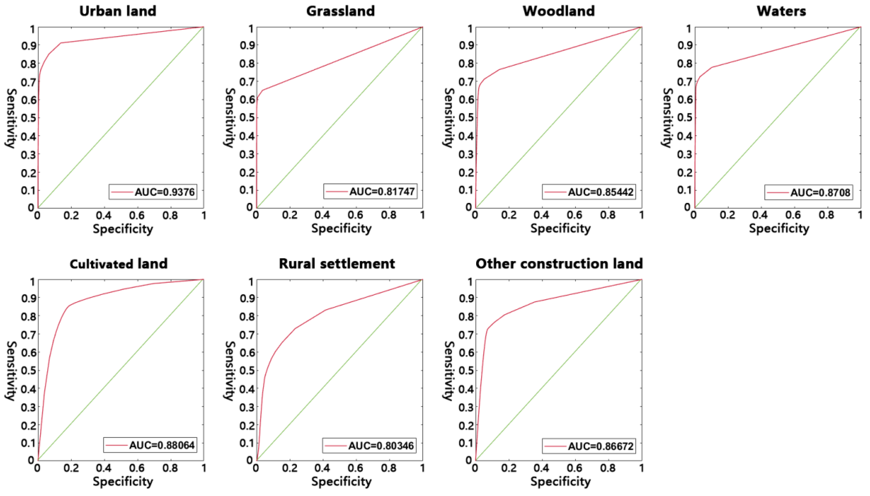
5.1. Model Performance
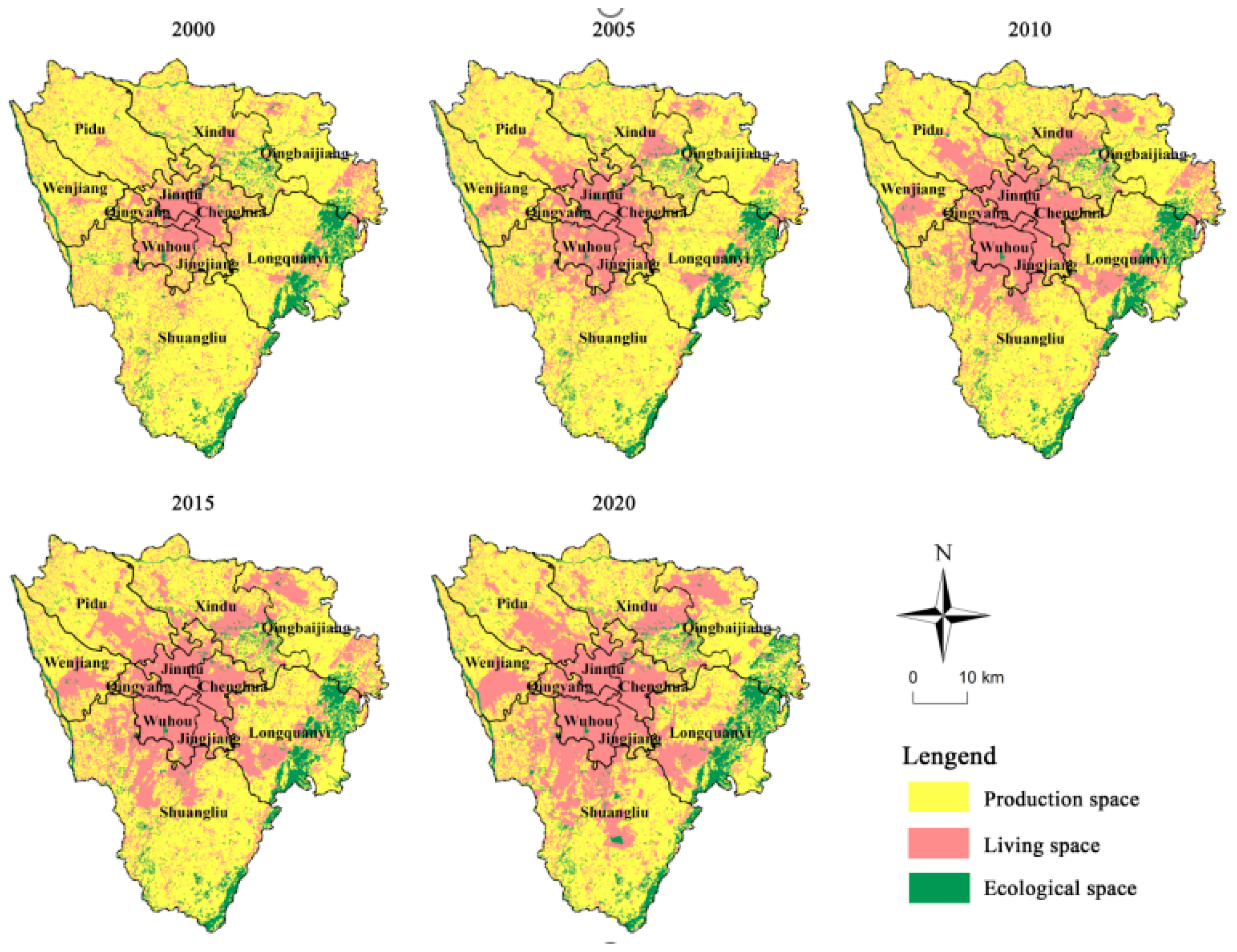
5.2. Analysis of the Evolution of the PLES
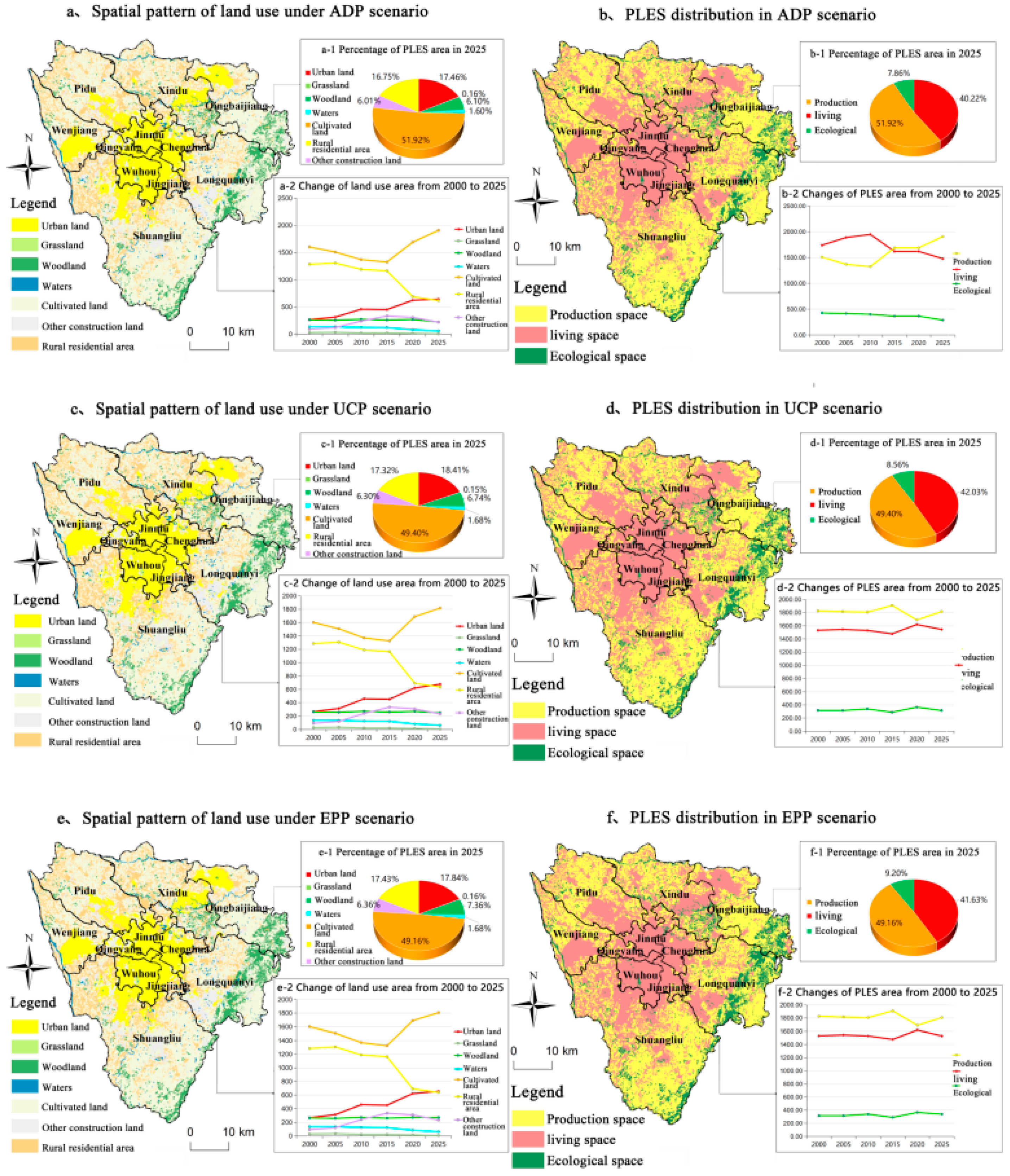
5.3. Multi-Scenario Simulation for 2025
6. Discussion
6.1. The General Law of Scenario Evolution
6.2. Discussion of the Multi-Scenario Simulation Model
7. Conclusions
Author Contributions
Funding
Institutional Review Board Statement
Informed Consent Statement
Data Availability Statement
Conflicts of Interest
Appendix A

| Primary Data Source | Data Classification | Data Processing and Usage | Year | Data Download |
|---|---|---|---|---|
| Geographical conditions | Geological disasters | Nuclear Density Analysis | 2020 | National Earth System Science Data Center |
| DEM | Slope and Aspect Analysis | 2010 | Geospatial Data Cloud | |
| Ecological environment | Ecological environmental quality | Extract Value to Point; Extract the ecological and environmental quality conditions of sample units | 2010/2015 | Resource and Environmental Sciences Data Center |
| Biodiversity | 2000/2005 | |||
| NPP | 2010/2020 | |||
| Farmland potential productivity | 2000/2010 | |||
| Soil erosion | 2010/2015 | |||
| Soil quality | 2015 | |||
| Water quality | 2015 | https://data.epmap.org/product/province_water (accessed on 14 January 2023) | ||
| NDVI | 2015/2020 | Geospatial Data Cloud | ||
| Climatic conditions | Temperature | Extract Value to Point; Extract climate change from sample units | 2010/2015/2020 | Resource and Environmental Sciences Data Center |
| Precipitation | 2010/2015/2020 | |||
| Built environment | POI | Nuclear Density Analysis; Extract the urban development and construction conditions | 2015/2020 | http://59.175.109.173:8888/index.html (accessed on 14 January 2023) |
| Nighttime light | Extract Value to Point; Extract the degree of economic development of sample unit | 2020 | https://www.arcgis.com/home/search.html?q=POI (accessed on 14 January 2023) | |
| Population density | 2010/2015/2020 | http://www.geodoi.ac.cn/WebCn/doi.aspx?Id=131 (accessed on 14 January 2023) | ||
| GDP | 2010/2015 | http://www.geodoi.ac.cn/WebCn/doi.aspx?Id=125 (accessed on 14 January 2023) | ||
| Distance factor | Neighbor Analysis; Extract the location advantage condition of the sample unit | 2010/2015/2020 | Resource and Environmental Sciences Data Center | |
| OpenStreetMap (http://www.openstreetmap.org/ (accessed on 14 January 2023)) | ||||
| Road integration | Space Syntax; Extracting the road accessibility of sample units | 2010/2015/2020 | ||
| Spatial location | Longitude | Extract the spatial location relationship of sample units | 2020 | Resource and Environmental Sciences Data Center |
| Latitude | ||||
| Land use | Land use in historical period | Extract the historical land type of the sample unit | 2000/2005/2010/2015/2020 |
References
- United Nations. World Urbanization Prospects; (The 2011 Revision); United Nations: New York, NY, USA, 2012. [Google Scholar]
- Wang, Q.; Yuan, X.; Zhang, J.; Gao, Y.; Hong, J.; Zuo, J.; Liu, W. Assessment of the Sustainable Development Capacity with the Entropy Weight Coefficient Method. Sustainability 2015, 7, 13542–13563. [Google Scholar] [CrossRef] [Green Version]
- Wang, Q.; Zhang, X.; Wu, Y.; Skitmore, M. Collective land system in China: Congenital flaw or acquired irrational weakness? Habitat Int. 2015, 50, 226–233. [Google Scholar] [CrossRef]
- Ye, C.; Chen, M.; Chen, R.; Guo, Z. Multi-scalar separations: Land use and production of space in Xianlin, a university town in Nanjing, China. Habitat Int. 2014, 42, 264–272. [Google Scholar] [CrossRef]
- Adam, Y.O.; Pretzsch, J.; Darr, D. Land use conflicts in central Sudan: Perception and local coping mechanisms. Land Use Policy 2015, 42, 1–6. [Google Scholar] [CrossRef]
- Fu, B.J.; Tian, H.Q.; Tao, F.L.; Zhao, W.W.; Wang, S. Progress of the impact of global change on ecosystem services. China Basic Sci. 2020, 3, 25–30. [Google Scholar]
- Jianjun, J.I.N.; Chong, J.; Lun, L.I. The economic valuation of cultivated land protection: A contingent valuation study in Wenling City, China. Landsc. Urban Plan. 2013, 119, 158–164. [Google Scholar] [CrossRef]
- Li, Z.J.; Ma, X.D.; Sun, S.S. Coupling analysis of rural transformation and land use change in Northern Jiangsu: A case study of Peixian county. J. Jiangsu Norm. Univ. 2015, 33, 36–39. [Google Scholar]
- Liu, T.; Liu, H.; Qi, Y. Construction land expansion and cultivated land protection in urbanizing China: Insights from national land surveys, 1996–2006. Habitat Int. 2015, 46, 13–22. [Google Scholar] [CrossRef]
- Deines, J.M.; Schipanski, M.E.; Golden, B.; Zipper, S.C.; Nozari, S.; Rottler, C.; Guerrero, B.; Sharda, V. Transitions from irrigated to dryland agriculture in the Ogallala Aquifer: Land use suitability and regional economic impacts. Agric. Water Manag. 2020, 233, 106061. [Google Scholar] [CrossRef]
- Li, J.; Sun, W.; Li, M.; Linlin, M. Coupling coordination degree of production, living and ecological spaces and its influencing factors in the Yellow River Basin. J. Clean. Prod. 2021, 298, 126803. [Google Scholar] [CrossRef]
- Ouyang, Z.; Zheng, H.; Xiao, Y.; Polasky, S.; Liu, J.; Xu, W.; Wang, Q.; Zhang, L.; Xiao, Y.; Rao, E.; et al. Improvements in ecosystem services from investments in natural capital. Science 2016, 352, 1455–1459. [Google Scholar] [CrossRef]
- Wiggering, H.; Müller, K.; Werner, A.; Helming, K. The Concept of Multifunctionality in Sustainable Land Development. In Sustainable Development of Multifunctional Landscapes; Helming, K., Wiggering, H., Eds.; Springer: Berlin/Heidelberg, Germany, 2003; pp. 3–18. [Google Scholar]
- Hao, Q. Reconstructing the value of territorial spatial planning for ecological civilization. Econ. Geogr. 2022, 42, 146–153. [Google Scholar]
- Hao, Q.; Liang, H.; Yang, K.; Feng, Z.; Wang, X.; Lu, Q. Innovation in the theory and technical methods of territorial spatial planning in the era of ecological civilization. J. Nat. Resour. 2022, 37, 2763–2773. [Google Scholar]
- Wang, H.; Zhu, F. Site selection model of land consolidation projects based on multi-objective optimization PSO. Trans. Chin. Soc. Agric. Eng. 2015, 31, 255–263. [Google Scholar]
- Li, X.; Li, D.; Liu, X.; He, J.Q. Geographical Simulation and Optimization System (GeoSOS) and Its Cutting-edge Researches. Adv. Earth Sci. 2009, 24, 899–907. [Google Scholar]
- Kilicoglu, C.; Cetin, M.; Aricak, B.; Sevik, H. Integrating multicriteria decision-making analysis for a GIS-based settlement area in the district of Atakum, Samsun, Turkey. Theor. Appl. Climatol. 2021, 143, 379–388. [Google Scholar] [CrossRef]
- Liu, J.L.; Liu, Y.S.; Li, Y.R. Classification evaluation and spatial-temporal analysis of “production-living-ecological” spaces in China. Acta Geogr. Sin. 2017, 72, 1290–1304. [Google Scholar]
- Chen, Y.M.; Liu, Z.H.; Zhou, B.B. Population-environment dynamics across world’s top 100 urban agglomerations: With implications for transitioning toward global urban sustainability. J. Environ. Manag. 2022, 319, 115630. [Google Scholar] [CrossRef]
- Li, H.; Fang, C.; Xia, Y.; Liu, Z.; Wang, W. Multi-Scenario Simulation of Production-Living-Ecological Space in the Poyang Lake Area Based on Remote Sensing and RF-Markov-FLUS Model. Remote. Sens. 2022, 14, 2830. [Google Scholar] [CrossRef]
- Jin, G.; Guo, B.; Cheng, J.; Deng, X.; Wu, F. A framework of spatial layout and support system of national land based on resource efficiency. J. Geogr. 2022, 77, 534–546. [Google Scholar]
- Li, D.; Hu, G.; Li, X.; Liu, X.; Ding, G.; Cai, Y. Delineating Urban Development Boundaries (UDBs) by Coupling Geographical Simulation and Spatial Optimization. China Land Sci. 2020, 34, 104–114. [Google Scholar]
- Zhang, Y.; Ou, M.H.; Jin, X.W.; Guo, J. Research on the Methord of Evaluating the Implementation of General Land Use Planning. China Land Sci. 2011, 25, 40–46. [Google Scholar]
- Chen, Y.M.; Li, X. Application and new trends of machine learning in urban spatial evolution simulation. J. Wuhan Univ. (Inf. Sci. Ed.) 2020, 45, 1884–1889. [Google Scholar]
- Cai, C.; Shu, B.; Zhu, H.; Yuan, X.; Yong, X. A simulation model of land use change driven by regional heterogeneity. China Land Sci. 2020, 34, 38–47. [Google Scholar]
- Li, F.X. An agent-based learning-embedded model (ABM-learning) for urban land use planning: A case study of residential land growth simulation in Shenzhen, China. Land Use Policy 2020, 95, 104620. [Google Scholar] [CrossRef]
- Ning, J.; Liu, J.; Kuang, W.; Xu, X.; Zhang, S.; Yan, C.; Li, R.; Wu, S.; Hu, Y.; Du, G.; et al. Spatiotemporal patterns and characteristics of land-use change in China during 2010–2015. J. Geogr. Sci. 2018, 28, 547–562. [Google Scholar] [CrossRef] [Green Version]
- Chen, Y.M.; Li, S.Y.; Li, X.; Liu, X.P. Simulating Compact Urban Form Using Cellular Automata (CA) and Multi-criteria Evaluation. Acta Sci. Nat. Univ. Sunyatsen 2010, 49, 110–114. [Google Scholar]
- Fan, J.; Wang, Q.; Wang, Y.; Chen, D.; Zhou, K. Assessment of coastal development policy based on simulating a sustainable land-use scenario for Liaoning Coastal Zone in China. Land Degrad. Dev. 2018, 29, 2390–2402. [Google Scholar] [CrossRef]
- Guzman, L.A.; Escobar, F.; Peña, J.; Cardona, R. A cellular automata-based land-use model as an integrated spatial decision support system for urban planning in developing cities: The case of the Bogotá region. Land Use Policy 2020, 92, 104445. [Google Scholar] [CrossRef]
- Mamanis, G.; Vrahnakis, M.; Chouvardas, D.; Nasiakou, S.; Kleftoyanni, V. Land Use Demands for the CLUE-S Spatiotemporal Model in an Agroforestry Perspective. Land 2021, 10, 1097. [Google Scholar] [CrossRef]
- Safitri, S.; Wikantika, K.; Riqqi, A.; Deliar, A.; Sumarto, I. Spatial Allocation Based on Physiological Needs and Land Suitability Using the Combination of Ecological Footprint and SVM (Case Study: Java Island, Indonesia). ISPRS Int. J. Geo-Inf. 2021, 10, 259. [Google Scholar] [CrossRef]
- Clarke, K.C.; Johnson, J.M. Calibrating SLEUTH with big data: Projecting California’s land use to 2100. Comput. Environ. Urban Syst. 2020, 83, 101525. [Google Scholar] [CrossRef]
- Edan, M.H.; Maarouf, R.M.; Hasson, J. Predicting the impacts of land use/land cover change on land surface temperature using remote sensing approach in Al Kut, Iraq. Phys. Chem. Earth Parts A/B/C 2021, 123, 103012. [Google Scholar] [CrossRef]
- Huang, J.; Lin, H.; Qi, X. A literature review on optimization of spatial development pattern based on ecological-production-living space. Prog. Geogr. 2017, 36, 378–391. [Google Scholar]
- Li, G.; Fang, C. Quantitative function identification and analysis of urban ecological-production-living spaces. Acta Geogr. Sin. 2016, 71, 49–65. [Google Scholar]
- Xi, J.; Wang, S.; Zhang, R. Restructuring and Optimizing Production-Living-Ecology Space in Rural Settlements. J. Nat. Resour. 2016, 31, 425–435. [Google Scholar]
- Zhang, H.Q.; Xu, E.Q.; Zhu, H.Y. An ecological-living-industrial land classification system and its spatial distribution in China. Resour. Sci. 2015, 37, 1332–1338. [Google Scholar]
- Cui, J.; Gu, J.; Sun, J.; Luo, J. The Spatial Pattern and Evolution Characteristics of the Production, Living and Ecological Space in Hubei Provence. China Land Sci. 2018, 32, 67–73. [Google Scholar]
- Jin, X.; Lu, Y.; Lin, J.; Qi, X.; Hu, G.; Li, X. Research on the evolution of spatiotemporal patterns of production-livingecological space in an urban agglomeration in the Fujian Delta region. China Acta Ecol. Sin. 2018, 38, 4286–4295. [Google Scholar]
- Xiao, C.; Ou, M.H.; Li, X. Research on spatial optimum allocation of construction land in an eco-economic comparative advantage perspective:a case study of Yangzhou City. Acta Ecol. Sin. 2015, 35, 696–708. [Google Scholar]
- Yang, H.L.X. Study on Village Type Identification Based on Spatial Evolution and Simulation of “Production-Living-Ecological Space”: A Case Study of Changning City in Hunan Province. China Land Sci. 2020, 34, 18–27. [Google Scholar]
- Chuvieco, E. Integration of linear programming and GIS for land-use modelling. Int. J. Geogr. Inf. Syst. 1993, 7, 71–83. [Google Scholar] [CrossRef]
- Chen, Y.; Li, X.; Liu, X.; Huang, H.; Ma, S. Simulating urban growth boundaries using a patch-based cellular automaton with economic and ecological constraints. Int. J. Geogr. Inf. Sci. 2019, 33, 55–80. [Google Scholar] [CrossRef]
- Jin, G.G.B.; Chen, J.; Deng, X.; Wu, F. Layout optimization and support system of territorial space: An analysis framework based on resource efficiency. Acta Geogr. Sin. 2022, 77, 534–546. [Google Scholar]
- Liu, X.; Liang, X.; Li, X.; Xu, X.; Ou, J.; Chen, Y.; Li, S.; Wang, S.; Pei, F. A future land use simulation model (FLUS) for simulating multiple land use scenarios by coupling human and natural effects. Landsc. Urban Plan. 2017, 168, 94–116. [Google Scholar] [CrossRef]
- Liang, X.Y.; JIN, X.B.; Sun, R.; Han, B.; Ren, J.; Zhou, Y.K. China’s resilience-space for cultivated land protection under the restraint of muti-scenario food security bottom line. Acta Geogr. Sin. 2022, 77, 697–713. [Google Scholar]
- Su, Y.Q.; Liu, G.; Zhao, J.B.; Niu, J.J.; Zhang, E.Y.; Guo, L.G.; Lin, F. Multi-scenario simulation prediction of ecological space in Fenhe River Basin using the FLUS model. Arid. Zone Res. 2021, 38, 1152–1161. [Google Scholar]
- Ou, M.H.; Ding, G.Q.; Guo, J.; Liu, Q. Multi-objective collaborative governance mechanism of territorial space planning. China Land Sci. 2020, 34, 8–17. [Google Scholar]
- Breiman, L. Bagging predictors. Mach. Learn. 1996, 24, 123–140. [Google Scholar] [CrossRef] [Green Version]
- Chandra, S.; Maheshkar, S. Verification of static signature pattern based on random subspace, REP tree and bagging. Multimed. Tools Appl. 2017, 76, 19139–19171. [Google Scholar] [CrossRef]
- Galar, M.; Fernandez, A.; Barrenechea, E.; Bustince, H.; Herrera, F. A Review on Ensembles for the Class Imbalance Problem: Bagging-, Boosting-, and Hybrid-Based Approaches. IEEE Trans. Syst. Man Cybern. Part C Appl. Rev. 2011, 42, 463–484. [Google Scholar] [CrossRef]
- Pant, S.; Lombardi, D. An information-theoretic approach to assess practical identifiability of parametric dynamical systems. Math. Biosci. 2015, 268, 66–79. [Google Scholar] [CrossRef] [Green Version]
- Chen, Y.; Li, X.; Liu, X.; Zhang, Y.; Huang, M. Tele-connecting China’s future urban growth to impacts on ecosystem services under the shared socioeconomic pathways. Sci. Total Environ. 2019, 652, 765–779. [Google Scholar] [CrossRef]
- Chen, Y.; Liu, X.; Li, X. Calibrating a Land Parcel Cellular Automaton (LP-CA) for urban growth simulation based on ensemble learning. Int. J. Geogr. Inf. Sci. 2017, 31, 2480–2504. [Google Scholar] [CrossRef]
- Wang, S.; Qu, Y.; Zhao, W.; Guan, M.; Ping, Z. Evolution and Optimization of Territorial-Space Structure Based on Regional Function Orientation. Land 2022, 11, 505. [Google Scholar] [CrossRef]
- Li, T.; Long, H.; Liu, Y.; Tu, S. Multi-scale analysis of rural housing land transition under China’s rapid urbanization: The case of Bohai Rim. Habitat Int. 2015, 48, 227–238. [Google Scholar] [CrossRef]
- Zacharias, J.; Lei, Y. Villages at the urban fringe—The social dynamics of Xiaozhou. J. Rural Stud. 2016, 47, 650–656. [Google Scholar] [CrossRef]
- Cao, M.; Chang, L.; Ma, S.; Zhao, Z.; Wu, K.; Hu, X.; Gu, Q.; Lv, G.; Chen, M. Multi-Scenario Simulation of Land Use for Sustainable Development Goals. IEEE J. Sel. Top. Appl. Earth Obs. Remote Sens. 2022, 15, 2119–2127. [Google Scholar] [CrossRef]
- Zhou, L.; Dang, X.; Sun, Q.; Wang, S. Multi-scenario simulation of urban land change in Shanghai by random forest and CA-Markov model. Sustain. Cities Soc. 2020, 55, 102045. [Google Scholar] [CrossRef]
- Zhao, X.; Li, S.; Pu, J.; Miao, P.; Wang, Q.; Tan, K. Optimization of the National Land Space Based on the Coordination of Urban-Agricultural-Ecological Functions in the Karst Areas of Southwest China. Sustainability 2019, 11, 6752. [Google Scholar] [CrossRef] [Green Version]
- Hou, Y.; Zhou, S.; Burkhard, B.; Müller, F. Socioeconomic influences on biodiversity, ecosystem services and human well-being: A quantitative application of the DPSIR model in Jiangsu, China. Sci. Total Environ. 2014, 490, 1012–1028. [Google Scholar] [CrossRef] [PubMed]
- Lyu, R.; Zhang, J.; Xu, M.; Li, J. Impacts of urbanization on ecosystem services and their temporal relations: A case study in Northern Ningxia, China. Land Use Policy 2018, 77, 163–173. [Google Scholar] [CrossRef]
- Thebo, A.L.; Drechsel, P.; Lambin, E.F. Global assessment of urban and peri-urban agriculture: Irrigated and rainfed croplands. Environ. Res. Lett. 2014, 9, 114002. [Google Scholar] [CrossRef]
- Wu, J.; Zhang, D.; Wang, H.; Li, X. What is the future for production-living-ecological spaces in the Greater Bay Area? A multi-scenario perspective based on DEE. Ecol. Indic. 2021, 131, 108171. [Google Scholar] [CrossRef]
- Baró, F.; Palomo, I.; Zulian, G.; Vizcaino, P.; Haase, D.; Gómez-Baggethun, E. Mapping ecosystem service capacity, flow and demand for landscape and urban planning: A case study in the Barcelona metropolitan region. Land Use Policy 2016, 57, 405–417. [Google Scholar] [CrossRef] [Green Version]
- Long, H.; Qu, Y. Land use transitions and land management: A mutual feedback perspective. Land Use Policy 2018, 74, 111–120. [Google Scholar] [CrossRef]
- Plieninger, T.; Bieling, C.; Fagerholm, N.; Byg, A.; Hartel, T.; Hurley, P.; López-Santiago, C.A.; Nagabhatla, N.; Oteros-Rozas, E.; Raymond, C.M.; et al. The role of cultural ecosystem services in landscape management and planning. Curr. Opin. Environ. Sustain. 2015, 14, 28–33. [Google Scholar] [CrossRef] [Green Version]
- Schwaab, J.; Deb, K.; Goodman, E.; Lautenbach, S.; van Strien, M.; Grêt-Regamey, A. Reducing the loss of agricultural productivity due to compact urban development in municipalities of Switzerland. Comput. Environ. Urban Syst. 2017, 65, 162–177. [Google Scholar] [CrossRef]
- Dupras, J.; Marull, J.; Parcerisas, L.; Coll, F.; Gonzalez, A.; Girard, M.; Tello, E. The impacts of urban sprawl on ecological connectivity in the Montreal Metropolitan Region. Environ. Sci. Policy 2016, 58, 61–73. [Google Scholar] [CrossRef] [Green Version]
- Ogle, J.; Delparte, D.; Sanger, H. Quantifying the sustainability of urban growth and form through time: An algorithmic analysis of a city’s development. Appl. Geogr. 2017, 88, 1–14. [Google Scholar] [CrossRef]
- Meiyappan, P.; Dalton, M.; O’Neill, B.C.; Jain, A.K. Spatial modeling of agricultural land use change at global scale. Ecol. Model. 2014, 291, 152–174. [Google Scholar] [CrossRef] [Green Version]
- Hurtt, G.C.; Chini, L.P.; Frolking, S.; Betts, R.A.; Feddema, J.; Fischer, G.; Fisk, J.P.; Hibbard, K.; Houghton, R.A.; Janetos, A.; et al. Harmonization of land-use scenarios for the period 1500–2100: 600 years of global gridded annual land-use transitions, wood harvest, and resulting secondary lands. Clim. Chang. 2011, 109, 117. [Google Scholar] [CrossRef] [Green Version]
- Sleeter, B.M.; Sohl, T.L.; Bouchard, M.A.; Reker, R.R.; Soulard, C.E.; Acevedo, W.; Griffith, G.E.; Sleeter, R.R.; Auch, R.F.; Sayler, K.L.; et al. Scenarios of land use and land cover change in the conterminous United States: Utilizing the special report on emission scenarios at ecoregional scales. Glob. Environ. Chang. 2012, 22, 896–914. [Google Scholar] [CrossRef] [Green Version]
- Rounsevell, M.D.A.; Reginster, I.; Araújo, M.B.; Carter, T.R.; Dendoncker, N.; Ewert, F.; House, J.I.; Kankaanpää, S.; Leemans, R.; Metzger, M.J.; et al. A coherent set of future land use change scenarios for Europe. Agric. Ecosyst. Environ. 2006, 114, 57–68. [Google Scholar] [CrossRef]
- Verburg, P.H.; Kok, K.; Pontius, R.G.; Veldkamp, A. Modeling Land-Use and Land-Cover Change. In Land-Use and Land-Cover Change: Local Processes and Global Impacts; Lambin, E.F., Geist, H., Eds.; Springer: Berlin/Heidelberg, Germany, 2006; pp. 117–135. [Google Scholar]
- Wang, T.; Jiang, Z.; Zhao, B. Health co-benefits of achieving sustainable net-zero greenhouse gas emissions in California. Nat. Sustain. 2020, 3, 597–605. [Google Scholar] [CrossRef]
- Ehsan, E.; Zainab, K.; Muhammad, Z.T.; Zhang, H.X.; Xing, L. Extreme weather events risk to crop-production and the adaptation of innovative management strategies to mitigate the risk: A retrospective survey of rural Punjab, Pakistan. Technovation 2022, 117, 102255. [Google Scholar]
- Ehsan, E.; Zainab, K. Estimating smart energy inputs packages using hybrid optimisation technique to mitigate environmental emissions of commercial fish farms. Appl. Energy 2022, 326, 119602. [Google Scholar]
- Eckhardt, K.; Breuer, L.; Frede, H.-G. Parameter uncertainty and the significance of simulated land use change effects. J. Hydrol. 2003, 273, 164–176. [Google Scholar] [CrossRef]
- Prestele, R.; Alexander, P.; Rounsevell, M.D.A.; Arneth, A.; Calvin, K.; Doelman, J.; Eitelberg, D.A.; Engström, K.; Fujimori, S.; Hasegawa, T.; et al. Hotspots of uncertainty in land-use and land-cover change projections: A global-scale model comparison. Glob. Chang. Biol. 2016, 22, 3967–3983. [Google Scholar] [CrossRef] [PubMed] [Green Version]
- Verburg, P.H.; Tabeau, A.; Hatna, E. Assessing spatial uncertainties of land allocation using a scenario approach and sensitivity analysis: A study for land use in Europe. J. Environ. Manag. 2013, 127, S132–S144. [Google Scholar] [CrossRef] [PubMed]
- Han, B.; Jin, X.; Xiang, X.; Rui, S.; Zhang, X.; Jin, Z.; Zhou, Y. An integrated evaluation framework for Land-Space ecological restoration planning strategy making in rapidly developing area. Ecol. Indic. 2021, 124, 107374. [Google Scholar] [CrossRef]
- Wilhelm, J.A.; Smith, R.G.; Jolejole-Foreman, M.C.; Hurley, S. Resident and stakeholder perceptions of ecosystem services associated with agricultural landscapes in New Hampshire. Ecosyst. Serv. 2020, 45, 101153. [Google Scholar] [CrossRef]
- Hagenauer, J.; Helbich, M. Local modelling of land consumption in Germany with RegioClust. Int. J. Appl. Earth Obs. Geoinf. 2018, 65, 46–56. [Google Scholar] [CrossRef]


| Scenario | Instructions | Core Land Space | Target | Reference |
|---|---|---|---|---|
| Scenario 1: Agricultural development priority (ADP) | Give maximum protection to arable land and strictly control the conversion of basic cultivated to other types of land. | Production space Cultivated land | Controls the quality and quantity of cultivated to ensure food security. | [48] |
| Scenario 2: Urban construction priority (UCP) | Make full use of living space to maximize the economic benefits of scale. | Living space Urban land; Rural settlements; Other construction land | Reveals the core driving force and potential threat to social stability and ecological environment under the priority city development mode. | [49] |
| Scenario 3: Ecological protection priority (EPP) | Set the maximum ecological space capacity to ensure the maximum ecological benefits provided by land use. | Ecological space Woodland; Grassland; Water area | Provides reference value for the delineation of ecological red line and promotes high-quality urban development. | [50] |
| Sce 1 | Living Space | Sce 2 | Ecological Space | Sce 3 | Production Space | |||||||||||
|---|---|---|---|---|---|---|---|---|---|---|---|---|---|---|---|---|
| Urban Land | W | Other Construction Land | W | Rural Settlements | W | Wood Land | W | Grassland | W | Water Area | W | Cultivated Land | W | |||
| UCP | Farmland productivity potential | 0.128 | Farmland productivity potential | 0.128 | Biological richness | 0.137 | EPP | Biological richness | 0.137 | Farmland productivity potential | 0.128 | Night light | 0.090 | ADP | NDVI | 0.093 |
| Ecological environmental quality | 0.104 | Soil erosion | 0.094 | Night light | 0.090 | GDP | 0.109 | GDP | 0.109 | Ecological environmental quality | 0.104 | Temperature | 0.036 | |||
| Biological richness | 0.137 | Precipitation | 0.061 | Ecological environmental quality | 0.104 | Farmland productivity potential | 0.128 | NDVI | 0.093 | NDVI | 0.093 | POP | 0.071 | |||
| GDP | 0.109 | GDP | 0.109 | NPP | 0.077 | POP | 0.071 | POP | 0.071 | Farmland productivity potential | 0.128 | NPP | 0.077 | |||
| Night light | 0.090 | NDVI | 0.093 | POP | 0.071 | Soil erosion | 0.094 | Ecological environmental quality | 0.104 | GDP | 0.109 | GDP | 0.109 | |||
| NPP | 0.077 | Biological richness | 0.137 | GDP | 0.109 | NPP | 0.077 | Night light | 0.090 | Soil erosion | 0.094 | Night light | 0.090 | |||
| Land Use Types | Actual Land Use in 2020 | |||||||
|---|---|---|---|---|---|---|---|---|
| Urban Land | Grassland | Woodland | Water Area | Cultivated Land | Other Construction Land | Rural Settlements | Total | |
| Urban land | 42,731 | 323 | 249 | 282 | 3970 | 3914 | 4455 | 55,924 |
| Grassland | 111 | 685 | 70 | 16 | 146 | 71 | 165 | 1264 |
| Woodland | 108 | 11 | 15,966 | 111 | 4417 | 3509 | 506 | 24,628 |
| Water area | 194 | 4 | 159 | 4895 | 1666 | 200 | 447 | 7565 |
| Cultivated land | 1675 | 21 | 3679 | 1107 | 130,503 | 5269 | 11,153 | 153,407 |
| Other construction land | 1950 | 33 | 628 | 297 | 9699 | 12,856 | 2227 | 27,690 |
| Rural settlements | 890 | 22 | 573 | 242 | 13,111 | 2472 | 45,013 | 62,323 |
| Territorial Space Structure | Area (km2) | Dynamic Degree (%) | ||||||||
|---|---|---|---|---|---|---|---|---|---|---|
| 2000 | 2005 | 2010 | 2015 | 2020 | 2000 –2005 | 2005 –2010 | 2010 –2015 | 2015 –2020 | 2000 –2020 | |
| Production space | 1602.20 | 1508.74 | 1369.90 | 1325.64 | 1689.87 | −1.17% | −1.84% | −0.65% | 5.50% | 0.27% |
| Living space | 1644.85 | 1739.98 | 1888.53 | 1948.17 | 1619.97 | 1.16% | 1.71% | 0.63% | −3.37% | −0.08% |
| Ecological space | 428.28 | 426.62 | 416.91 | 401.54 | 365.50 | −0.08% | −0.46% | −0.74% | −1.80% | −0.73% |
Disclaimer/Publisher’s Note: The statements, opinions and data contained in all publications are solely those of the individual author(s) and contributor(s) and not of MDPI and/or the editor(s). MDPI and/or the editor(s) disclaim responsibility for any injury to people or property resulting from any ideas, methods, instructions or products referred to in the content. |
© 2023 by the authors. Licensee MDPI, Basel, Switzerland. This article is an open access article distributed under the terms and conditions of the Creative Commons Attribution (CC BY) license (https://creativecommons.org/licenses/by/4.0/).
Share and Cite
Cao, Q.; Tang, J.; Huang, Y.; Shi, M.; van Rompaey, A.; Huang, F. Modeling Production-Living-Ecological Space for Chengdu, China: An Analytical Framework Based on Machine Learning with Automatic Parameterization of Environmental Elements. Int. J. Environ. Res. Public Health 2023, 20, 3911. https://doi.org/10.3390/ijerph20053911
Cao Q, Tang J, Huang Y, Shi M, van Rompaey A, Huang F. Modeling Production-Living-Ecological Space for Chengdu, China: An Analytical Framework Based on Machine Learning with Automatic Parameterization of Environmental Elements. International Journal of Environmental Research and Public Health. 2023; 20(5):3911. https://doi.org/10.3390/ijerph20053911
Chicago/Turabian StyleCao, Qi, Junqing Tang, Yudie Huang, Manjiang Shi, Anton van Rompaey, and Fengjue Huang. 2023. "Modeling Production-Living-Ecological Space for Chengdu, China: An Analytical Framework Based on Machine Learning with Automatic Parameterization of Environmental Elements" International Journal of Environmental Research and Public Health 20, no. 5: 3911. https://doi.org/10.3390/ijerph20053911