A Causal Analysis of Life Expectancy at Birth. Evidence from Spain


Department of Economics and Business, Universidad de Almería, 04120 Almería, Spain
*
Author to whom correspondence should be addressed.
Int. J. Environ. Res. Public Health 2019, 16(13), 2367; https://doi.org/10.3390/ijerph16132367
Submission received: 12 June 2019
/
Revised: 26 June 2019
/
Accepted: 30 June 2019
/
Published: 3 July 2019
(This article belongs to the Special Issue Mathematical and Statistical Models in Environmental Research and Public Health with Applications)
Abstract
:Background: From a causal point of view, there exists a set of socioeconomic indicators concerning life expectancy. The objective of this paper is to determine the indicators which exhibit a relation of causality with life expectancy at birth. Methods: Our analysis applies the Granger causality test, more specifically its version by Dumitrescu–Hurlin, starting from the information concerning life expectancy at birth and a set of socioeconomic variables corresponding to 17 Spanish regions, throughout the period 2006–2016. To do this, we used the panel data involving the information provided by the Spanish Ministry of Health, Consumer Affairs and Social Welfare (MHCSW) and the National Institute of Statistics (NIS). Results: Per capita income, and the rate of hospital beds, medical staff and nurses Granger-cause the variable “life expectancy at birth”, according to the Granger causality test applied to panel data (Dumitrescu–Hurlin’s version). Conclusions: Life expectancy at birth has become one of the main indicators able to measure the performance of a country’s health system. This analysis facilitates the identification of those factors which exhibit a unidirectional Granger-causality relationship with life expectancy at birth. Therefore, this paper provides useful information for the management of public health resources from the point of view of the maximization of social benefits.
1. Introduction
Life expectancy at birth has become an aggregate variable which reflects the influence of a wide variety of indicators (social, economic, environmental, etc.) [1] on the working of modern health systems. On the other hand, the current complex health context, characterized by the constant interrelation of a large number of variables of different types, motivates the causal analysis of these variables which can indicate, among other aspects, the degree to which the resources available to public authorities contribute to the efficient performance of health policies.
A review of the existing literature on this topic (see Section 2) shows that, to the extent of our knowledge, no papers have opted to employ a causal analysis. At this point, it is necessary to clarify that sometimes correlation seems to be confused with causality, which is an obvious error of appreciation which, in statistics, is called the fallacy cum hoc ergo propter hoc, that is to say, a priori, that correlation does not necessarily imply causality [2]. On other occasions, although the causal analysis is properly contextualized by performing the “classic” Granger causality test for panel data (stacked pairwise Granger causality test), the analysis is not always focused on the variable “life expectancy”, but rather on the causal relationship between GDP per capita and health expenditure per capita [3]. Therefore, the research question is to address a causal approach to the determinants of health outcome by applying, for the first time in this field, the methodology put forward by Dumitrescu–Hurlin for panel data [4]. This novel procedure is a non-homogeneous causality test, that is to say, a causal empirical analysis which considers the possible correlation of ten socioeconomic variables with the variable “life expectancy at birth” during the period 2006–2016, in the context of the seventeen Spanish regions.
Spain, like Great Britain and Italy, uses a variation of the Beveridge model. In this system, the government provides and finances health care, through taxes. Currently, Spain has a decentralized health system under national coordination. Since 2002, the organization and delivery of health services have been transferred to the seventeen regional health administrations.
This study seeks to examine the causal link between life expectancy at birth and some health care resources and socio-economic factors in the aforementioned Spanish regions from 2006 to 2016. Our contribution is to identify whether the parameters of hospital beds, medical staff in specialized care, medical staff in primary care, nursing staff in specialized care, nursing staff in primary care (all above expressed per 1000 inhabitants), and per capita income are Granger causal for the variable “life expectancy at birth” according to the Granger causality test for panel data (longitudinal, multi-dimensional data involving measurements over time) (Dumitrescu–Hurlin version). This result is of great importance for the design of health policies in our country since, in principle, it highlights the factors which it is necessary to influence in order to increase the level of life expectancy at birth in Spain.
2. Literature Review
A review of the empirical literature on this subject reveals the existence of studies which analyze the main determinants of life expectancy using a global approach and macroeconomic data. This type of research analyzes the total effect of the use of health care on the health status of citizens and thereby indicates the implications of different economic policies. Focusing our attention on works which follow a macro approach as referred to developed countries, we classify the determinants of the health status of the population in three categories, namely socio-economic factors, health resources, and lifestyle-related factors. With respect to the socio-economic factors, almost all works consider gross domestic product or per capita income [5,6,7], and with less frequency some indicator of income distribution [8,9,10]. Unemployment is also analyzed [11,12,13] as a determinant of the health status of the population as a representative measure of the fluctuations of the economic cycle. Other relevant macroeconomic variables used in this type of analysis are inflation [14] and gross capital [15].
Education is frequently included in these analyses [16,17,18] as well as the level of employment [5,6,19]. Among demographic variables, some works include the age of the population, i.e., the percentage of those over 60 or 65 [20,21].
Within the category of socioeconomic factors, some works include variables of an institutional nature such as the type of health system [22,23] or the level of fiscal decentralization, corruption and political rights [24]. Another factor which has been incorporated into this type of analysis is pollution, generally represented by emissions of polluting substances [2,6,15,19,25] or by some environmental quality indicator [26]. Recently, existing literature has been enriched by introducing globalization [27] and some indicators of social development [28] as possible determinants of health status.
Regarding health resources, it is common to use some expression of health expenditure. In this way, we can consider either the total expenditure [21,29,30], the entire component of public health expenditure [6,9,19,31], or public and private health expenditure separately [32]. Other authors have incorporated other items such as expenditure on pharmaceutical products [33,34,35] and various categories of other social expenditure in order to assess their differential effect on health status [36,37,38]. Part of this literature also incorporated some proxy variables of health resources (mainly doctors and nurses [19,29]) and, less frequently, the number of beds [31,38]. Additionally, medical innovation [39] (measured by the use of innovative medicines) and the requirement of having a medical prescription for the consumption of certain medications [40] have been analyzed as conditioning factors of the health status.
In order to identify the effects of health habits and lifestyle, it is usual in this type of literature to include other specific variables such as the consumption of tobacco and alcohol, and others concerning diet, such as the intake of vegetables, fruits, sugar, butter, calories, fats, proteins, or even the level of obesity. Within this group of works, we can highlight the papers by [29,30,31,33,34,41].
In Spain, we can find some works on the determinants of the health status from a microeconomic point of view [42]. On the other hand, a regional setting has been employed in other papers but dealing with the efficiency of the Spanish health system [43,44,45]. However, our paper occupies an intermediate position with respect to the former studies, since our aim is to analyze the determinants of the Spanish health system by using macro data of Spanish regions.
In addition, [46] investigate at a regional level and by using aggregate data, the effect of decentralization on health care outcomes in Spain by testing whether a greater decentralization is linked to improvements in population health between 1992 and 2003. To do this, they use infant mortality and life expectancy as dependent variables. They find that income, decentralization, and health care resources have an important influence on both infant mortality and life expectancy. In the same line, [47] analyzes the relationship between unemployment and mortality by using data from some Spanish provinces during the period 1980–1997.
3. Materials and Methods
One of the extensions of the well-known Granger causality test [48] is its possible application to panel data starting from a fixed effects model [49] (known as the stacked pairwise Granger causality test):
where and are the observations of two stationary variables corresponding to an individual i in a period t and with a number of delays K exactly the same for all individuals. The null hypothesis in this model is:
which states the equality of coefficients corresponding to the N individuals included in the panel, that is to say, derived from all cross-sectional observations.
However, the previous way of conceptualizing Granger’s causality, restricted to panel data, has some weaknesses related to the viability of such a test [50] which depends on the selected number of items N within a given time horizon T. [51,52], or its adequacy or, more correctly, the functionality (or working schema) of the null hypothesis (2) since, when considering that a variable causes another in a data panel, it is assumed that a null hypothesis has been added to that already proposed [53].
To overcome these drawbacks, Dumitrescu and Hurlin [4] designed a homogeneous non-causality test, derived from (1), in which a balanced panel composed of and , that is to say, by observing two stationary variables corresponding to an individual i in a period t and with a number of delays K exactly the same for all individuals, it is possible to violate the “classical” assumption (heterogeneous causality test) by assuming that coefficients , being invariant with respect to time, can differ among individuals, thus leading to a new null and alternative hypothesis:
It should be observed that the alternative hypothesis establishes the plausible causality between the variables and for some individuals, but not for all of them, so the rejection of does not necessarily imply the existence of causality among some individuals [54]. This hypothesis is known as the hypothesis of homogeneous non-causality and differs from (2) in that the alternative hypothesis allows the causality between and for some individuals, but not for all.
Nevertheless, the contrast of hypothesis (3) is formulated under the assumption that, in the case of a causal relationship given a set of N items, the vectors must be strictly identical when adding, as an alternative hypothesis, the existence of () items over which there is no a priori explicit causal relationship. Dumitrescu and Hurlin [4] resolve these drawbacks by determining the standard regressions of the Granger causality for each individual in order to obtain the individual Wald statistics and, starting from there, calculate the statistic (average Wald or W-bar):
where is the Wald statistic applied to the i-th individual in t, which corresponds with the null hypothesis . Analogously, taking into account the hypothesis that the calculated Wald statistics are independent and identically distributed for each of the individuals, it can be demonstrated that the standardized statistics follow a standard normal distribution, when T and N tend to infinity and K denotes the selected number of lags:
Moreover, given a fixed dimension of T, with , the estimated standardized statistic also follows a standard normal distribution:
This last aspect determines the number of delays or lags which must be selected for the Dumitrescu and Hurlin homogeneous non-causality test [12], although originally these authors did not specify a given or optimal number of delays [54], whereby a viable solution may be the combined use of estimators derived from the information criteria by Akaike or Hannan-Quinn, and the Bayesian analysis. However, in our particular study, we have implemented only one time-lag because we were constrained by in order that the Wald statistics could be independently distributed with finite second order moments. In other words, since we are using a time horizon of 11 years, K had to be one taking into account the aforementioned restriction (condition that, given the database used in our work, would be violated with two or more lags).
Finally, the contrast of the null hypothesis in (3) is made according to the values of and , by comparing them with the standard critical values, rejecting the null hypothesis and therefore concluding that there is causality in the Granger sense according to the procedure of Dumitrescu and Hurlin [4] when or are greater than the standard critical values, taking into account that, for panel data in which N and T are relatively large, it is more appropriate to test the null hypothesis by means of , leaving the use of for those cases where N is relatively large and T is relatively small.
Given the aforementioned defined variables, we are going to propose the following model in which the subscripts i and t denote, respectively, the different Spanish regions and the period corresponding to the analyzed time horizon (2006–2016):
where , and where represents the random perturbation of the model ().
Instead of carrying out a prototypical econometric analysis focused on the unit root test, the cointegration or the estimation of the long-term coefficients of the model previously stated (i.e., through the Dynamic Ordinary Least Squares (D-OLS) and Fully Modified Ordinary Least Squares (F-MOLS) procedures), we are going to focus on the analysis of stationarity of the time series included in the panel data and on the implementation of the Granger causality test by Dumitrescu–Hurlin for panel data. With respect to stationarity, this analysis is prescriptive given that, in the Granger causality test, the analyzed time series must be stationary by definition. At this point, it is necessary to indicate that there is no single statistical test which automatically corroborates the stationarity of the series. In order to draw different conclusions based on whether or not these tests show relatively similar results, more than one stationarity test is usually applied. In this way, we have only applied the Im–Pesaran–Shin (IPS) test, taking advantage of its simplicity and its relatively easy interpretation.
However, among all existing stationarity tests for panel data such as Levin–Lin–Chu (LLC test), Maddala–Wu (MW test), Breitung (test B) and IPS test [55], we have opted for the latter because it leads to the elimination of the serial correlation of the analyzed variables, having a large capacity in relatively small samples [56] such as the one used in this paper.
On the other hand, the IPS test is an ad hoc stationarity test for the implementation of the procedure by Dumitrescu–Hurlin, given that it considers the heterogeneity between the different cross sections. An important characteristic of this test is that it facilitates that the values of (autoregressive coefficients) vary indistinctly between the sections in the panel, by allowing some series, but not necessarily all of them, to be stationary.
The hypothesis contrast of the IPS test is formulated as follows:
from where it can be derived that the null hypothesis represents the existence of a unitary root, meaning no presence of stationarity in data. This hypothesis will be rejected (considering that the series is stationary in at least one cross-section of the panel), by comparing the value of the statistic t and the probabilistic critical values provided by the IPS test.
Finally, it is necessary to emphasize that, although this test has recognized a bidirectional contrast in which the variable “life expectancy” could act both as cause and effect, we opted for a unidirectional contrast in which this variable is the exclusive cause of the different explanatory variables listed above. The bidirectionality, in this specific case, would be completely illogical.
With respect to the methodology proposed in this paper, we have tried to look for an ad hoc implementation of the causality in Granger by taking into account the nature of the data used (panel data). In order to contextualize this research, it is convenient to indicate how the causality in Granger represents an analytical framework which has evolved since its original definition [48] expressly focused on time series and linear causality until multiple revisions and readjustments.
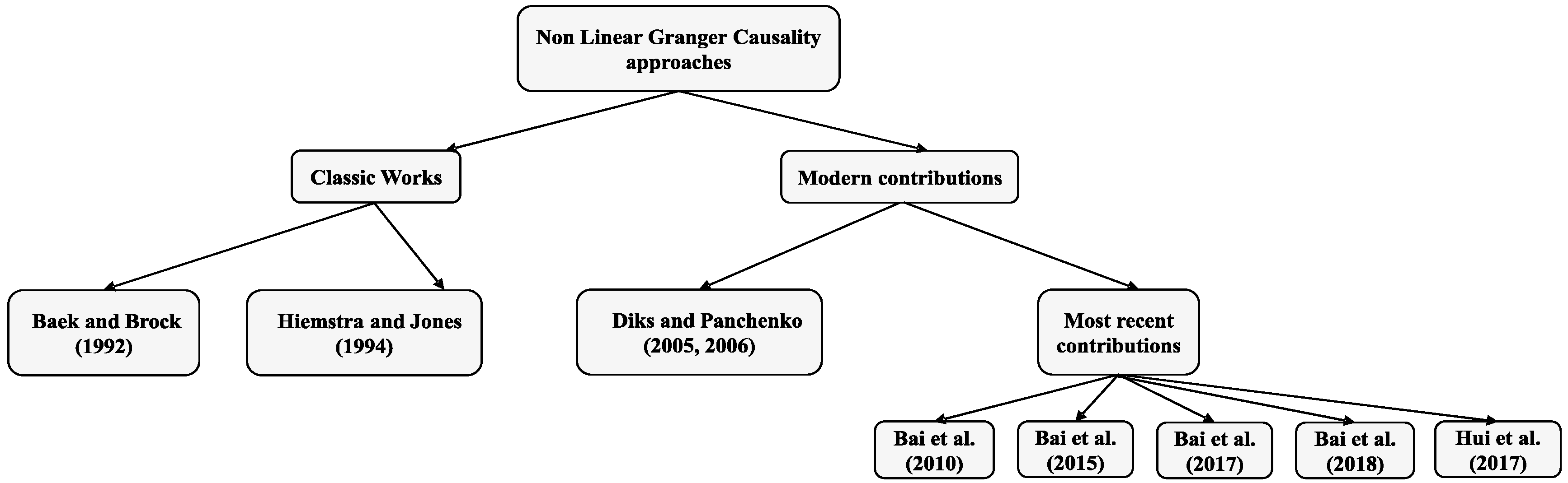
One of the revisions of the scheme originally drawn up by [48] starts from inferring that the plausible causal relationship between two variables, if any, would hardly be strictly linear in nature [57]. The adequacy of Granger causality in the field of non-linearity is one of the big fields in which research has been diversified, showing the Figure 1 a brief summary of the most notable works focused on non-linear Granger causality:
Properly speaking, the non-linear causality analysis of Granger began with [58], and was subsequently readjusted by [59], a transcendental contribution in this field which for more than ten years would guide most of non-linear causal analyses in which both causal approaches, linear and non-linear relationship (in the sense of Granger) between the price and trading volumes of the New York Stock Exchange (NYSE) studied. The fundamental scheme of the nonlinear causality of [59], on which most of subsequent investigations would be based, is focused on the determination of a central limit theorem (CLT) of its statistic test by implementing the asymptotical properties of multivariate U-statistics.
[60] demonstrate, by using Monte Carlo simulations, that the lack of consistency is the main failure in the estimators used in the procedure designed by [59], by proposing, alternatively, a new non-parametric causal test and including a series of practical guidelines for nonparametric Granger causality testing. Consequently, [61] design an extension of the Diks and Panchenko test [60] which is applied to the US grain market. This test is characterized because it applies the data-sharpening as a bias reduction method.
[62] also choose to revise the non-linear test of [59], by suggesting new estimators of the probabilities in order to improve its asymptotic properties in accordance with the original procedure included in [59]. In the same way, [63] also review the non-linear test by [59] by constructing a novel nonlinear causality test in multivariate settings. [64] present a test contemplating different lags of variables and [65], taking [59] as reference, recalculate the probabilities and rebuild the CLT of the new statistic test, by concluding how their estimates are more consistent than the one shown in [59].
Finally, [66] create a completely original methodology to quickly, efficiently, and effectively analyze the nonlinear causal relationship given a group of variables, based on the particularity (also the advantage) that it is not required as a rule to know the exact nonlinear features and the detailed non-linear forms of the variable .
Obviously, once the non-linear field of causality in Granger was described in a very brief way, we would have to highlight three works whose practical implementation could greatly support our study: [65,66,67], especially if they are compared and put into perspective with the results obtained by the Dumitrescu–Hurlin procedure. However, if these non-linear causality approaches have not been applied in this work, it is simply due to reasons of operative nature, derived from the little data which compose our database.
In the first case [64], it would be quite difficult to employ a variable number of lags whilst in the following two papers [65,66] we presume that, for the same reasons, the results were not as robust and consistent as they should be, not because of any weakness of these causal models of proven efficacy (see, for example, the application of [66] in the SP index), but to the small size of the database used. In effect, in our opinion, any of these three works would be of great importance as a new methodological perspective in the causal analysis of life expectancy, opting for the nonlinear perspective, always more representative than the strictly linear one (see [57]).
4. Data
In our analysis, we have used panel data for the period 2006–2016 referred to life expectancy at birth and another ten socioeconomic variables closely related to it, the description of which is presented in Table 1. Thus, a database has been configured composed of 3179 observations, that is to say, 17 annual observations of the dependent and independent variables for each of the 17 Spanish regions.
The selection of these variables has been made based on the existing literature on this topic, which shows some consensus in considering health resources, socioeconomic factors, and lifestyle as determinants of health status. Unfortunately, in this work it has not been possible to include some variables representative of lifestyle, such as the percentage of smokers or drinkers, among others, as such information for each Spanish region is not available for the analyzed period. This lack of availability for the analyzed period also explains that the territorialized health expenditure has not been included. However, other health resources which are financed by this type of expenditure, namely personnel (doctors and nurses), or materials (hospital beds) have been considered.
5. Results
Table 3 shows the result of the IPS test of the different variables included in this analysis, in levels and first differences, by considering a single delay of the variables and under the assumption that, in the test equation, both the individual intercept and the trend of each series are included. It can be observed that, for most analyzed variables, the null hypothesis is rejected, which supports the property of stationarity in levels and first differences, except for a small number of variables indicated with an asterisk.
6. Discussion
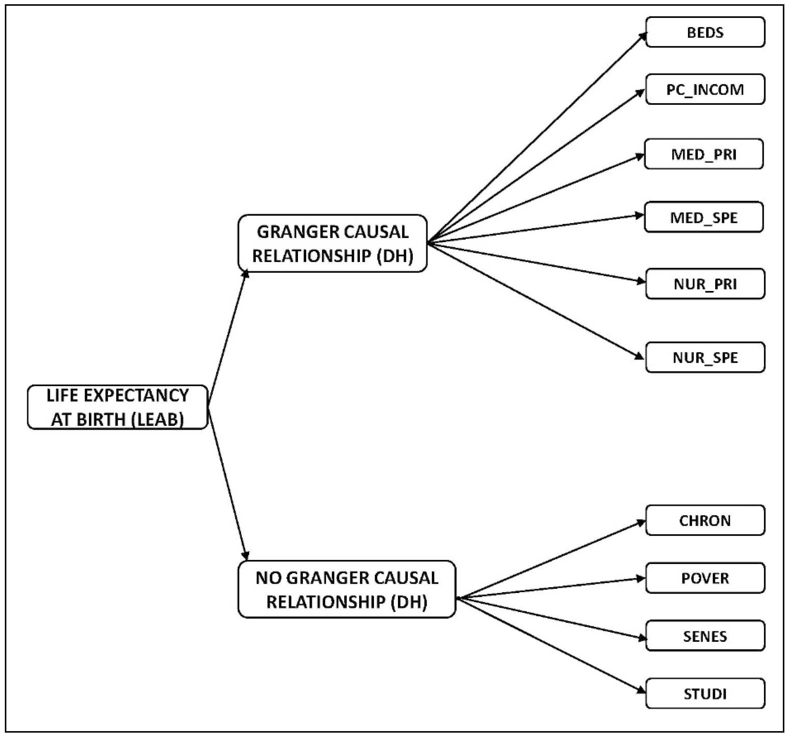
This research has analyzed the socioeconomic indicators which have exhibited a relation of causality with the life expectancy at birth in Spanish regions. Our findings have concluded that, according to the Granger causality test for panel data (Dumitrescu–Hurlin version), the explanatory variables hospital beds, medical staff in specialized care, medical staff in primary care, nursing staff in specialized care, nursing staff in primary care (all above expressed per 1000 inhabitants), and per capita income cause the variable “life expectancy at birth”. This result is very important for the design of health policies in Spain as it identifies the main factors to which it is necessary to give attention in order to increase the life expectancy at birth.
This study is aimed at contributing to the progress of research on health status determinants. Part of existing literature has included resources in physical terms such as the number of physicians and, to a lesser extent, the availability of nurses. An advantage of our analysis is that we have incorporated both personal resources to overcome this restriction in part of the empirical evidence since nurses also occupy an important place in the provision of health care.
Our results confirm previous researches since the number of doctors was found to be significant in improving health outcomes [2,29,31]. Specifically, our findings coincide with previous studies carried out in Spain which explore the determinants of life expectancy, in particular the contribution by [46] which differs from our approach in the following items:
- [46] also incorporate infant mortality as a dependent variable.
- These scholars also use fiscal decentralization as an explanatory variable.
- Finally, our paper is more exhaustive as it incorporates new independent variables such as people with long-term disease or health problems, poverty rate, level of studies, and senescence.
With respect to the methodology employed, our perspective is causal whilst [46] use panel data with fixed vs. random effects. Additionally, logarithms have been applied over the two dependent variables and real per capita income and the number of general practitioners.
More recently, some authors have suggested that health care development (measured by input indicators such as the number of hospital beds and the number of doctors per 1000 inhabitants, among others) could significantly improve life expectancy at birth [28]. However, other researchers have concluded that longevity is not explained by the amount of health care provisions, such as the number of hospital beds and the number of health care staff [38]. In addition, a previous study has revealed that, despite its (spurious) positive correlation, the availability of medical specialists has a low impact on mortality rates, in comparison with the economic and social variables which have been used as control variables [71]. On the other hand, in this type of literature, the impact of hospital beds in high-income countries is more ambiguous, and can be explained by the development of high-tech health care provisions which reduce the average length of hospitalization [7].
Whereas the role played by health care resources is more debated in existing literature, there is some consensus in concluding that socioeconomic and lifestyle factors [7] are important determinants of the population’s health status. One of the major socioeconomic factors which has been considered in the literature of life expectancy, is income. At this point, our results are consistent with previous studies showing the importance of income in improving life expectancy at birth [18,72,73,74].
7. Conclusions
The main contribution of this paper is threefold. On the one hand, it is the first time that the Granger causality test (Dumitrescu–Hurlin version) has been applied to a causal analysis within the health sector. This contribution becomes more relevant if we take into account the few studies which analyze the causality of health outcome in a country [2]. In this sense, subsequent contributions partially confirm our results in a study carried out in Turkey (using data covering the period 1975–2015), where causality relationships were analyzed (according to Granger) between per capita health expenditure, the number of doctors per thousand inhabitants and life expectancy in different age segments, and also between their variations [75]. In this way, it is necessary to repeat that the presence of a correlation between two variables does not necessarily imply the existence of causality. Thus, a corroborated conclusion in the literature is the existence of a close relationship between medical consultation rates and life expectancy as the highest consultation rates are presented in countries with the highest life expectancy [76]. However, this simple correlation does not necessarily imply causality, since the totality of living standards can influence consultation rates and life expectancy.
Second, we contribute to the analysis of life expectancy from a regional perspective. In this sense, it is evident that some studies based on macro data to identify the determinants of health status, have been generalized at country level. However, those works carried out at state, regional or municipal level are less frequent, such as those referred to North American states [5,10,77], the provinces of Canada [29,35], Spain [47], and China [28]; and to Brazilian municipalities [78].
Third, we must point out that another added value of this paper is the use of panel data, which is essential when dealing with information based on different Spanish regions.
Most of the previous empirical research on the determinants of health status have considered some parameter of health care expenditure. One limitation of our work is that we have not included this monetary resource because it is not available for Spanish regions for the entire period 2006–2016. The main restriction of this paper lies in the limited number of available observations, which has resulted in a reduction of the number of delays to one. Despite this limitation, our research analysis provides a relevant contribution to the evaluation of the impact on health and a useful tool for its possible implementation in public health programs.
Finally and as future research, we intend to investigate this type of contrast by using a database with longer time horizon and by incorporating new possible explanatory factors of life expectancy at birth.
Author Contributions
The individual contribution of each author has been as follows: conceptualization, N.R.L.; methodology, software and validation, P.A.M.C.; writing, supervision and funding acquisition, S.C.R.
Funding
This research has been funded by the Spanish Ministry of Economy and Competitiveness, grant number DER2016-76053R.
Acknowledgments
We would like to thank the authors of the Granger causality test (DH), E.I. Dumitrescu (Université Paris Nanterre) and C. Hurlin (Université d’Orléans) as well as S. Weber (Université de Neuchâtel) for their wise advice which, to a great extent, has been taken into account in the writing of this work. We are very grateful for the valuable comments and suggestions offered by two anonymous referees.
Conflicts of Interest
The authors declare no conflict of interest.
References
- Ministry of Health, Social Policy and Equality. Informe anual del Sistema Nacional de Salud 2016. Informes, Estudios e Investigación. 2017. Available online: http://www.msssi.gob.es/estadEstudios/estadisticas/sisInfSanSNS/tablasEstadisticas/InfAnSNS.htm (accessed on 1 May 2019).
- Nixon, J.; Ulmann, P. The relationship between health care expenditure and health outcomes—Evidence and caveats for a causal link. Eur. J. Health Econ. 2006, 7, 7–18. [Google Scholar] [CrossRef] [PubMed]
- Erdil, E.; Yetkiner, I.H. The Granger-causality between health care expenditure and output: A panel data approach. Appl. Econ. 2009, 41, 511–518. [Google Scholar] [CrossRef]
- Dumitrescu, E.-I.; Hurlin, C. Testing for Granger non-causality in heterogeneous panels. Econ. Model. 2012, 29, 1450–1460. [Google Scholar] [CrossRef] [Green Version]
- Auster, R.; Levesoardln, I.; Sarachek, S. The production of health: An exploratory study. J. Hum. Resour. 1969, 4, 411–436. [Google Scholar] [CrossRef]
- Or, Z. Determinants of health outcomes in industrialised countries: A pooled, cross–country, time series analysis. OECD Econ. Stud. 2000, 30, 53–77. [Google Scholar]
- Joumard, I.; André, C.; Nicq, C. Health Care Systems: Efficiency and Institutions; OECD Economics Department Working Papers No. 769; OECD Publishing: Paris, France, 2010. [Google Scholar]
- Rodgers, G.B. Income and inequality as determinants of mortality: An international cross–sectional analysis. Popul. Stud. 1979, 33, 343–351. [Google Scholar] [CrossRef]
- Berger, M.; Messer, J. Public financing of health expenditure, insurance, and health outcomes. Appl. Econ. 2002, 34, 2105–2113. [Google Scholar] [CrossRef]
- Hill, T.D.; Jorgenson, A. Bring out your dead!: A study of income inequality and life expectancy in the United States, 2000–2010. Health Place 2018, 49, 1–6. [Google Scholar] [CrossRef]
- McAvinchey, I.D. A comparison of unemployment, income and mortality interaction for five European countries. Appl. Econ. 1988, 20, 453–471. [Google Scholar] [CrossRef]
- Laporte, A. Do economic cycles have a permanent effect on population health? Revisiting the Brener hypothesis. Health Econ. 2004, 13, 767–779. [Google Scholar] [CrossRef]
- Shing–Jong, L. Economic fluctuations and health outcome: A panel analysis of Asia–Pacific countries. Appl. Econ. 2009, 41, 519–530. [Google Scholar]
- Bai, R.; Wei, J.; An, R.; Li, Y.; Collett, L.; Dang, S.; Dong, W.; Wang, D.; Fang, Z.; Zhao, Y.; et al. Trends in Life Expectancy and Its Association with Economic Factors in the Belt and Road Countries-Evidence from 2000–2014. Int. J. Environ. Res. Public Health 2018, 15, 2890. [Google Scholar] [CrossRef] [PubMed]
- Monsef, A.; Mehrjardi, A.S. Determinants of life expectancy: A panel data approach. Asian Econ. Financ. Rev. 2015, 5, 1251–1257. [Google Scholar] [CrossRef]
- Self, S.; Grabowski, R. How effective is public health expenditure in improving overall health? A cross–country analysis. Appl. Econ. 2003, 35, 835–845. [Google Scholar] [CrossRef]
- Cutler, D.M.; Lleras–Muney, A. Education and Health: International Comparisons; NBER Working Paper No. 17738; NBER: Cambridge, MA, USA, 2012. [Google Scholar]
- Ketenci, N.; Murthy, V.N.R. Some determinants of life expectancy in the United States: Results from cointegration tests under structural breaks. J. Econ. Financ. 2018, 42, 508–525. [Google Scholar] [CrossRef]
- Or, Z. Exploring the Effects of Health Care on Mortality Across OECD Countries; OECD Labour Market and Social Policy No. 46; Occasional Paper: Paris, France, 2000. [Google Scholar]
- Wolfe, B.L.; Gabay, M. Health status and medical expenditures: More evidence of a link. Soc. Sci. Med. 1987, 25, 883–888. [Google Scholar] [CrossRef]
- Hitiris, T.; Posnett, J. The determinants and effects of health expenditure in developed countries. J. Health Econ. 1992, 11, 173–181. [Google Scholar] [CrossRef]
- Elola, J.; Daponte, A.; Navarro, V. Health indicators and the organisation of health care systems in Western Europe. Am. J. Public Health 1995, 85, 1397–1401. [Google Scholar] [CrossRef] [PubMed]
- Grubaugh, S.G.; Rexford, E.S. Comparing the performance of health–care systems: An alternative approach. South. Econ. J. 1994, 60, 1030–1042. [Google Scholar] [CrossRef]
- Robalino, D.A.; Oscar, F.P.; Albertus, V. Does Fiscal Decentralization Improve Health Outcomes? Evidence from a Cross–Country Analysis; World Bank Policy Research Working Paper Series; The World Bank: Washington, DC, USA, 2001; Volume 2565, pp. 1–14. [Google Scholar]
- Al-Hemoud, A.; Gasana, J.; Al-Dabbous, A.N.; Al-Shatti, A.; Al-Khayat, A. Disability Adjusted Life Years (DALYs) in Terms of Years of Life Lost (YLL) Due to Premature Adult Mortalities and Postneonatal Infant Mortalities Attributed to PM2.5 and PM10 Exposures in Kuwait. Int. J. Environ. Res. Public Health 2018, 15, 2609. [Google Scholar] [CrossRef]
- Mariani, F.; Pérez-Barahona, A.; Raffin, N. Life expectancy and the environment. J. Econ. Dyn. Control 2010, 34, 798–815. [Google Scholar] [CrossRef]
- Bergh, A.; Nilsson, T. Good for living? On the relationship between globalization and life expectancy. World Dev. 2010, 38, 1191–1203. [Google Scholar] [CrossRef]
- Jiang, J.; Luo, L.; Xu, P.; Wang, P. How does social development influence life expectancy? A geographically weighted regression analysis in China. Public Health 2018, 163, 95–104. [Google Scholar] [CrossRef] [PubMed]
- Crémieux, P.-Y.; Ouellette, P.; Pilon, C. Health care spending as determinants of health outcomes. Health Econ. 1999, 8, 627–639. [Google Scholar] [CrossRef]
- Heijink, R.; Koolman, X.; Westert, G.P. Spending more money, saving more lives? The relationship between avoidable mortality and healthcare spending in 14 countries. Eur. J. Health Econ. 2013, 14, 527–538. [Google Scholar] [CrossRef] [PubMed]
- Cochrane, A.L.; St Ledger, A.S.; Moore, F. Health service ‘input’ and mortality ‘output’ in developed countries. J. Epidemiol. Community Health 1978, 32, 200–205. [Google Scholar] [CrossRef]
- Linden, M.; Ray, D. Life expectancy effects of public and private health expenditures in OECD countries 1970–2012: Panel time series approach. Econ. Anal. Policy 2017, 56, 101–113. [Google Scholar] [CrossRef]
- Miller, R.D.; Frech, T. The Productivity of Health Care and Pharmaceuticals: Quality of Life, Cause; UC Santa Barbara Departmental Working Papers No. 12-02; University of California: Santa Barbara, CA, USA, 2002. [Google Scholar]
- Shaw, J.W.; Horrace, W.C.; Vogel, R.J. The determinants of life expectancy: An analysis of the OECD health data. South. Econ. J. 2005, 71, 768–783. [Google Scholar] [CrossRef]
- Crémieux, P.Y.; Mieilleur, M.C.; Ouellette, P.; Petit, P.; Zelder, P.; Potvin, K. Public and private pharmaceutical spending as determinants of health outcomes in Canada. Health Econ. 2005, 14, 107–116. [Google Scholar] [CrossRef] [PubMed]
- Bradley, E.H.; Elkins, B.R.; Herrin, J.; Elbel, B. Health and social services expenditures: Associations with health outcomes. BMJ Qual. Saf. 2011, 20, 826–831. [Google Scholar] [CrossRef] [PubMed]
- Reynolds, M.M.; Avendano, M. Social policy expenditures and life expectancy in high–income countries. Am. J. Prev. Med. 2017, 54, 72–79. [Google Scholar] [CrossRef] [PubMed]
- Van den Heuvel, W.J.A.; Olaroiu, M. How important are health care expenditures for life expectancy? A comparative, European analysis. J. Am. Med Dir. Assoc. 2017, 18, 276.e9–276.e12. [Google Scholar] [CrossRef] [PubMed]
- Lichtenberg, F.R. Sources of U.S. longevity increase, 1960–1997. Q. Rev. Econ. Financ. 2004, 44, 369–389. [Google Scholar] [CrossRef]
- Peltzman, S. Regulation and health: The case of mandatory prescriptions and an extension. Manag. Decis. Econ. 1987, 8, 41–46. [Google Scholar] [CrossRef]
- Halicioglu, F. Modeling life expectancy in Turkey. Econ. Model. 2011, 28, 2075–2082. [Google Scholar] [CrossRef] [Green Version]
- Regidor, E.; Calle, M.E.; Navarro, P.; Domínguez, V. Trends in the association between average income, poverty and income inequality and life expectancy in Spain. Soc. Sci. Med. 2003, 56, 961–971. [Google Scholar] [CrossRef]
- Herrero, L.; Martín, J.L.; López del Amo, M.P. Eficiencia técnica de los hospitales públicos y de las empresas públicas hospitalarias de Andalucía. Gac. Sanit. 2015, 29, 274–281. [Google Scholar] [CrossRef] [PubMed]
- Cordero, J.M.; Nuño-Solinís, R.; Orueta, J.F.; Polo, C.; del Río-Cámara, M.; Alonso-Morán, E. Evaluación de la eficiencia técnica de la atención primaria pública en el País Vasco, 2010–2013. Gac. Sanit. 2016, 30, 104–109. [Google Scholar] [CrossRef]
- Pérez-Romero, C.; Ortega-Díaz, M.I.; Ocaña-Riola, R.; Martín-Martín, J.L. Análisis de la eficiencia técnica en los hospitales del Sistema Nacional de Salud español. Gac. Sanit. 2017, 31, 108–115. [Google Scholar] [CrossRef]
- Cantarero, D.; Pascual, M. Analysing the impact of fiscal decentralization on health outcomes: Empirical evidence from Spain. Appl. Econ. Lett. 2008, 15, 109–111. [Google Scholar] [CrossRef]
- Tapia–Granados, J.A. Recessions and mortality in Spain, 1980–1997. Eur. J. Popul. 2005, 21, 393–422. [Google Scholar] [CrossRef]
- Granger, C.W.J. Investigating causal relations by econometric models and cross-spectral methods. Econometrica 1969, 37, 424–438. [Google Scholar] [CrossRef]
- Holtz-Eakin, D.; Newey, W.; Rosen, H. Estimating vector autoregressions with panel data. Econometrica 1988, 56, 1371–1395. [Google Scholar] [CrossRef]
- Campo, J.; Mendoza, H. Gasto público y crecimiento económico: Un análisis regional para Colombia, 1984–2012. Lecturas de Economía 2018, 88, 77–108. [Google Scholar] [CrossRef]
- Nickell, S. Biases in dynamic models with fixed effects. Econometrica 1981, 49, 1417–1426. [Google Scholar] [CrossRef]
- Hurlin, C.; Venet, B. Granger causality tests in panel data models with fixed coefficients. In Cahier de Recherche EURISCO; Université Paris IX Dauphine: Paris, France, 2001. [Google Scholar]
- Granger, C.W.J. Some aspects of causal relationships. J. Econom. 2003, 112, 69–71. [Google Scholar] [CrossRef]
- Lopez, L.; Weber, S. Testing for Granger Causality in Panel Data. Stata J. 2018, 17, 972–984. [Google Scholar] [CrossRef]
- Im, K.S.; Pesaran, M.H.; Shin, Y. Testing for unit roots in heterogeneous panels. J. Econom. 2003, 115, 53–74. [Google Scholar] [CrossRef]
- Wang, S.S.; Zhou, D.Q.; Zhou, P.; Wang, Q.W. CO2 emissions, energy consumption and economic growth in China: A panel data analysis. Energy Policy 2011, 39, 4870–4875. [Google Scholar] [CrossRef]
- Granger, C.W.J. Forecasting in Business and Economics, 2nd ed.; Emerald Group Publishing Limited: Bingley, UK, 1989. [Google Scholar]
- Baek, E.G.; Brock, W.A. A General Test for Nonlinear Granger Causality: Bivariate Model; Working Paper; Korea Development Institute and University of Wisconsin Madison: Seoul, Korea, 1992. [Google Scholar]
- Hiemstra, C.; Jones, J.D. Testing for linear and nonlinear Granger causality in the stock price-volume relation. J. Financ. 1994, 49, 1639–1664. [Google Scholar]
- Diks, C.; Panchenko, V. A Note on the Hiemstra-Jones test for Granger non-causality. Stud. Nonlinear Dyn. Econom. 2005, 9. [Google Scholar] [CrossRef]
- Diks, C.; Panchenko, V. A new statistic and practical guidelines for nonparametric Granger causality testing. J. Econ. Dyn. Control 2006, 30, 1647–1669. [Google Scholar] [CrossRef] [Green Version]
- Bai, Z.; Hui, Y.; Lv, Z.; Wong, W.-K.; Zhu, Z.-Z. The Hiemstra-Jones test revisited. arXiv 2017, arXiv:1701.03992. [Google Scholar]
- Bai, Z.; Wong, W.-K.; Zhang, B. Multivariate linear and nonlinear causality tests. Math. Comput. Simul. 2010, 81, 5–17. [Google Scholar] [CrossRef] [Green Version]
- Bai, Z.; Xie, W.; Wong, W.-K. Panel Non-Linear Causality Test. 2015. Available online: https://ssrn.com/abstract=2608388 (accessed on 25 June 2019).
- Bai, Z.; Hui, Y.; Jiang, D.; Lv, Z.; Wong, W.-K.; Zheng, S. A new test of multivariate nonlinear causality. PLoS ONE 2018, 13, e0185155. [Google Scholar] [CrossRef] [PubMed]
- Hui, Y.; Wong, W.-K.; Bai, Z.; Zhu, Z.-Z. A new nonlinearity test to circumvent the limitation of Volterra expansion with application. J. Korean Stat. Soc. 2017, 46, 365–374. [Google Scholar] [CrossRef] [Green Version]
- Ministry of Health, Consumer Affairs and Social Welfare. Key indicators of the National Health System. 2018. Available online: http://inclasns.msssi.es/ (accessed on 2 February 2019).
- National Institute of Statistics. Survey of Living Conditions. 2018. Available online: http://www.ine.es/dyngs/INEbase/es/operacion.htm?c=Estadistica_C&cid=1254736176807&menu=ultiDatos&idp=1254735976608 (accessed on 2 February 2019).
- National Institute of Statistics. Labor Force Statistics. 2018. Available online: http://www.ine.es/dyngs/INEbase/es/categoria.htm?c=Estadistica_P&cid=1254735976594 (accessed on 2 February 2019).
- National Institute of Statistics. Statistics of Continuous Register. 2018. Available online: http://www.ine.es/dyngs/INEbase/es/operacion.htm?c=Estadistica_C&cid=1254736177012&menu=ultiDatos&idp=1254734710990 (accessed on 2 February 2019).
- Young, F.W. An explanation of the persistent doctor-mortality association. J. Epidemiol. Community Health 2001, 55, 80–84. [Google Scholar] [CrossRef] [PubMed] [Green Version]
- Preston, S.H. The changing relation between mortality and level of economic development. Popul. Stud. 1975, 29, 484–490. [Google Scholar] [CrossRef]
- Pritchett, L.; Summers, H. Wealthier is healthier. J. Hum. Resour. 1996, 31, 841–868. [Google Scholar] [CrossRef]
- Bloom, D.E.; Canning, D. Commentary: The Preston curve 30 years on: Still sparking fire. Int. J. Epidemiol. 2007, 36, 498–499. [Google Scholar] [CrossRef]
- Arvas, M.A.; Torusdağ, M. The link between health care expenditure and life expectancy: Turkey (1975–2015). Int. J. Humanit. Soc. Sci. Invent. 2017, 6, 59–64. [Google Scholar]
- OECD/World Health Organization. Health at a Glance: Asia/Pacific 2014: Measuring Progress towards Universal Health Coverage; OECD Publishing: Paris, France, 2014. [Google Scholar]
- Thornton, J. Estimating a health production function for the US: Some new evidence. Appl. Econ. 2002, 34, 59–62. [Google Scholar] [CrossRef]
- Soares, R.R. Health and the evolution of welfare across Brazilian municipalities. J. Dev. Econ. 2007, 84, 590–608. [Google Scholar] [CrossRef] [Green Version]
Figure 1.
Non-linear Granger causality approaches summary. Source: Own elaboration.

Figure 2.
Causal relationships resulting from the causality test for panel data (Dumitrescu–Hurlin version). Source: Own elaboration.
Figure 2.
Causal relationships resulting from the causality test for panel data (Dumitrescu–Hurlin version). Source: Own elaboration.


Table 1.
Description of variables and their sources. Source: Own elaboration.
| Variable | Short Definition | Source |
|---|---|---|
| LEAB | Life expectancy at Barth | Key indicators of the National Health System [67] |
| CHRON | People with long-term disease or health problems (population percentage greater than or equal to 16 years) | Survey of Living Conditions [68] |
| PC_INCOM | Average net annual income per person and unit of consumption by autonomous communities (euros) | Survey of Living Conditions [68] |
| POVER | Poverty rate (%) | Key indicators of the National Health System [67] |
| STUDI | Level of studies: Population from 16 to 64 years with 2nd level of secondary and post-secondary, non-higher education (%) | Labor Force Statistics [69] |
| SENES | Senescence: Population percentage greater than or equal to 65 years | Statistics of Continuous Register [70] |
| MED_SPE | Medical staff in specialized care per 1000 inhabitants | Key indicators of the National Health System [67] |
| MED_PRI | Medical staff in primary care per 1000 inhabitants | Key indicators of the National Health System [67] |
| NUR_SPE | Nursing staff in specialized care per 1000 inhabitants | Key indicators of the National Health System [67] |
| NUR_PRI | Nursing staff in primary care per 1000 inhabitants | Key indicators of the National Health System [67] |
| BEDS | Hospital beds per 1000 inhabitants | Key indicators of the National Health System [67] |
Table 2.
Variables and summary statistics. Source: Own elaboration.
| Variables | |||||||||||
|---|---|---|---|---|---|---|---|---|---|---|---|
| LEAB | BEDS | NUR_SPE | NUR_PRI | CHRON | MED_SPE | MED_PRI | STUDI | POVER | PC_INCOM | SENES | |
| Mean | 82.46 | 3.24 | 3.25 | 0.66 | 29.26 | 1.84 | 0.78 | 23.70 | 20.13 | 10,542.05 | 17.74 |
| Median | 82.49 | 3.30 | 3.16 | 0.66 | 28.80 | 1.79 | 0.76 | 23.70 | 18.10 | 10,493.00 | 17.80 |
| Maximum | 85.22 | 4.35 | 4.93 | 0.89 | 45.90 | 2.55 | 1.10 | 29.70 | 40.20 | 14,838.00 | 24.10 |
| Minimum | 79.77 | 2.17 | 2.53 | 0.47 | 16.10 | 1.37 | 0.59 | 16.20 | 5.30 | 6668.00 | 12.10 |
| Std.Dev. | 1.12 | 0.49 | 0.50 | 0.10 | 5.87 | 0.23 | 0.10 | 2.56 | 7.73 | 1880.22 | 2.90 |
| Skewness | −0.19 | −0.49 | 1.02 | 0.36 | 0.22 | 0.62 | 1.37 | −0.34 | 0.44 | 0.27 | 0.22 |
| Kurtosis | 2.67 | 2.64 | 3.56 | 2.58 | 2.84 | 2.90 | 5.60 | 3.06 | 2.23 | 2.24 | 2.25 |
| Jarque-Bera test | 1.93 | 8.52 | 34.55 | 5.32 | 1.69 | 12.22 | 111.04 | 3.55 | 10.70 | 6.81 | 5.89 |
Table 3.
Stationarity test by Im–Pesaran–Shim for the analyzed sample. Source: Own elaboration.
| IPS Test Null Hypothesis: Unitary Root (Assumes the Process of Unitary Roots at an Individual Level) | ||||
|---|---|---|---|---|
| A. Levels | ||||
| Series | t-Statistic | Probability | Cross Sections | Observations |
| BEDS (*) | 1.58573 | 0.9436 | 17 | 153 |
| NUR_SPE | 0.65073 | 0.7424 | 17 | 153 |
| NUR_PRI | −2.00706 | 0.0224 | 17 | 153 |
| CHRON | −0.49536 | 0.3102 | 17 | 153 |
| LEAB (*) | 1.02956 | 0.8484 | 17 | 153 |
| MED_SPE | 0.19513 | 0.5774 | 17 | 153 |
| MED_PRI | −1.91310 | 0.0279 | 17 | 153 |
| STUDI | −2.00483 | 0.0225 | 17 | 153 |
| POVER | 0.37674 | 0.6468 | 17 | 153 |
| PC_INCOM | −4.19584 | 0.0000 | 17 | 153 |
| SENES | −0.83526 | 0.2018 | 17 | 153 |
| B. First Differences | ||||
| Series | t-Statistic | Probability | Cross Sections | Observations |
| BEDS | −0.56214 | 0.287 | 17 | 136 |
| NUR_SPE | −0.80952 | 0.2091 | 17 | 136 |
| NUR_PRI | −1.50039 | 0.0668 | 17 | 136 |
| CHRON | 0.03717 | 0.5148 | 17 | 136 |
| LEAB | −3.75752 | 0.0001 | 17 | 136 |
| MED_SPE | −0.60668 | 0.272 | 17 | 136 |
| MED_PRI | −1.2299 | 0.1094 | 17 | 136 |
| STUDI | −1.4124 | 0.0789 | 17 | 136 |
| POVER | −1.98178 | 0.0238 | 17 | 136 |
| PC_INCOM (*) | 1.9624 | 0.9187 | 17 | 136 |
| SENES | 0.60758 | 0.7283 | 17 | 136 |
(*) means that, for these variables, the null hypothesis is not rejected.
Table 4.
Causality test for panel data (Dumitrescu–Hurlin version) for the analyzed sample. Source: Own elaboration.
Table 4.
Causality test for panel data (Dumitrescu–Hurlin version) for the analyzed sample. Source: Own elaboration.
| Null Hypothesis | Wbar Statistic | Zbar Statistic | Probability |
|---|---|---|---|
| BED does not homogeneously cause LEAB | 1.92798 | 0.77748 | 0.4369 |
| NUR_SPE does not homogeneously cause LEAB | 2.22473 | 1.21445 | 0.2246 |
| NUR_PRI does not homogeneously cause LEAB | 2.00144 | 0.88564 | 0.3758 |
| CHRON does not homogeneously cause LEAB | 0.71378 | −1.01049 | 0.3123 |
| MED_SPE does not homogeneously cause LEAB | 3.31763 | 2.82378 | 0.0047 |
| MED_PRI does not homogeneously cause LEAB | 2.40673 | 1.48244 | 0.1382 |
| STUDI does not homogeneously cause LEAB | 1.12455 | −0.40561 | 0.685 |
| POVER does not homogeneously cause LEAB | 0.92645 | −0.69733 | 0.4856 |
| PC_INCOM does not homogeneously cause LEAB | 2.7489 | 1.98631 | 0.047 |
| SENES does not homogeneously cause LEAB | 0.50179 | −1.32265 | 0.186 |
© 2019 by the authors. Licensee MDPI, Basel, Switzerland. This article is an open access article distributed under the terms and conditions of the Creative Commons Attribution (CC BY) license (http://creativecommons.org/licenses/by/4.0/).
Share and Cite
MDPI and ACS Style
Martín Cervantes, P.A.; Rueda López, N.; Cruz Rambaud, S. A Causal Analysis of Life Expectancy at Birth. Evidence from Spain. Int. J. Environ. Res. Public Health 2019, 16, 2367. https://doi.org/10.3390/ijerph16132367
AMA Style
Martín Cervantes PA, Rueda López N, Cruz Rambaud S. A Causal Analysis of Life Expectancy at Birth. Evidence from Spain. International Journal of Environmental Research and Public Health. 2019; 16(13):2367. https://doi.org/10.3390/ijerph16132367
Chicago/Turabian StyleMartín Cervantes, Pedro Antonio, Nuria Rueda López, and Salvador Cruz Rambaud. 2019. "A Causal Analysis of Life Expectancy at Birth. Evidence from Spain" International Journal of Environmental Research and Public Health 16, no. 13: 2367. https://doi.org/10.3390/ijerph16132367
Note that from the first issue of 2016, this journal uses article numbers instead of page numbers. See further details here.