Article

Design of Potent Inhibitors Targeting the Main Protease of SARS-CoV-2 Using QSAR Modeling, Molecular Docking, and Molecular Dynamics Simulations

1
Laboratory of Molecular Chemistry, Department of Chemistry, Faculty of Sciences Semlalia, BP 2390, Marrakech 40000, Morocco
2
Laboratoire de Photochimie et d’Ingénierie Macromoléculaires (LPIM), Ecole Nationale Supérieure de Chimie de Mulhouse, Université de Haute-Alsace, 68100 Mulhouse, France
3
University Artois, CNRS, Centrale Lille, University Lille, UMR 8181, Unité de Catalyse et Chimie du Solide (UCCS), F-62300 Lens, France
4
African Genome Center, Mohammed VI Polytechnic University, Ben Guerir 43150, Morocco
*
Author to whom correspondence should be addressed.
Pharmaceuticals 2023, 16(4), 608; https://doi.org/10.3390/ph16040608
Submission received: 12 March 2023 / Revised: 8 April 2023 / Accepted: 14 April 2023 / Published: 18 April 2023
(This article belongs to the Special Issue Protease-Based Drug Discovery)

Abstract

:
Severe acute respiratory syndrome coronavirus 2 (SARS-CoV-2) infection is a serious global public health threat. The evolving strains of SARS-CoV-2 have reduced the effectiveness of vaccines. Therefore, antiviral drugs against SARS-CoV-2 are urgently needed. The main protease (Mpro) of SARS-CoV-2 is an extremely potent target due to its pivotal role in virus replication and low susceptibility to mutation. In the present study, a quantitative structure–activity relationship (QSAR) study was performed to design new molecules that might have higher inhibitory activity against SARS-CoV-2 Mpro. In this context, a set of 55 dihydrophenanthrene derivatives was used to build two 2D-QSAR models using the Monte Carlo optimization method and the Genetic Algorithm Multi-Linear Regression (GA-MLR) method. From the CORAL QSAR model outputs, the promoters responsible for the increase/decrease in inhibitory activity were extracted and interpreted. The promoters responsible for an increase in activity were added to the lead compound to design new molecules. The GA-MLR QSAR model was used to ensure the inhibitory activity of the designed molecules. For further validation, the designed molecules were subjected to molecular docking analysis and molecular dynamics simulations along with an absorption, distribution, metabolism, excretion, and toxicity (ADMET) analysis. The results of this study suggest that the newly designed molecules have the potential to be developed as effective drugs against SARS-CoV-2.

1. Introduction

Three years after the emergence of the COVID-19 disease caused by severe acute respiratory syndrome coronavirus 2 (SARS-CoV-2), the entire world is still suffering from the major health and socioeconomic consequences of the disease [1]. Accordingly, significant research efforts have been made to develop vaccines and drugs to effectively stop COVID-19. However, SARS-CoV-2 continues to claim human lives due to frequent mutations in its viral genome that make the new variants more transmissible and infectious, such as B.1.1.7 (alpha), B.1.351 (beta), B.1.617.2 (delta), and B.1.1.529 (omicron) [2,3,4,5]. Therefore, the discovery of new inhibitors that work better at different stages of SARS-CoV-2 propagation has become a priority.
SARS-CoV-2 is an enveloped positive-stranded RNA virus that, once it enters the cell, translates the single-stranded RNA into two large polyproteins known as pp1a and pp1ab that mediate viral replication and propagation [6]. During viral maturation, most cleavage events are controlled by a nonstructural protein 5 (nsp5), also known as the main protease (Mpro or 3CLpro), which is in charge of 11 different cleavages in the early stages of viral replication [7]. Mpro is an attractive target due to: (i) its pivotal role in viral replication and maturation [8]; (ii) minor mutations that have occurred in its genomic sequence in the new variants of SARS-CoV-2 compared to other major proteins, [9] and (iii) its inhibitors that are unlikely to be dangerous as no human proteases with similar cleavage specificity have been identified [10]. The Mpro monomer consists of three domains: domain I, domain II, and domain III, which include amino acid residues 8–101, 102–184, and 201–306, respectively [11]. Despite the fact that each individual monomeric component has its own active site, the Mpro of SARS-CoV-2 is enzymatically active only as a homodimer [11,12,13]. Therefore, it might be logical to block the catalytic site (CS) and dimer interface site (DIS) to inhibit the main function of the protease and its dimerization.
In continuation of our efforts to develop new potent Mpro inhibitors [14], in this study, two quantitative structure–activity relationships (QSAR) were developed based on the structural properties of dihydrophenanthrene derivatives and their inhibitory activities against Mpro. The first model, based on Monte Carlo optimization, was used to build SMILES-based QSAR models that provide insights into the design of new Mpro inhibitors. The second model used the genetic algorithm multi-linear regression approach (GA-MLR) to confirm the prediction of the inhibitory activity of the designed molecules. Since the dihydrophenanthrene derivative could inhibit SARS-CoV-2 by targeting the CS and DIS of the Mpro, a molecular docking study was carried out to investigate the interaction of the designed molecules within the CS and DIS of Mpro. In addition, the most potent designed molecules were subjected to molecular dynamics simulations in order to investigate their stability and behavior within the CS and DIS sites of Mpro. An absorption, distribution, metabolism, excretion, and toxicity (ADMET) evaluation of these molecules was also performed.

2. Results and Discussions

2.1. CORAL QSAR Model

Six QSAR models were built based on three random splits and two target functions: TF1 with WIIC = 0 and TF2 with WIIC = 0.2. Three splits were created from the entire dataset and each split was divided into four sets, as described below (for definitions of the parameters, refer to the Materials and Methods section (Section 3) of this article). The obtained statistical parameters for the developed SMILES-based QSAR models show that WIIC = 0.2 increases the effect of IIC on Monte Carlo optimization. Table 1 displays the computed statistical parameters for all splits. Figure 1 depicts the experimental pIC50 values compared to the estimated values for the three splits. Table 1 clearly illustrates that all models are statistically reliable and fulfill the criteria set by Tropsha et al. [15] and Ojha et al. [16]. All data points of the three splits are in the applicability domain as shown in the Supplementary Materials in Table S1. The QSAR model with a higher R2 value for the validation set and a higher IIC value for the calibration set was selected as the leading model. Therefore, the QSAR model of split 2 had the highest R2 value of 0.9203 for the validation set and a higher IIC value of 0.9277 for the calibration set. The numerical values of the various parameters for the validation set of split 2 were Q2 = 0.8508, CCC = 0.9157, r2m = 0.8825, and Δr2m = 0.0647. The split 2 model is as follows in Equation (1):
pIC 50 = 1.7915330   ± 0.04504500 + 0.0672532   ± 0.0010114 × DCW 3 , 17

2.2. GA-MLR QSAR Model

The GA-MLR method was applied to the training set and then evaluated to the test set using the six selected descriptors that contribute to the inhibitory activity (Table 2). The GA-MLR model Equation (2) and its statistical parameters are presented below:
pIC 50 = 0.5833   ×   Eig 09 _ AEA dm     0.018   ×   P _ VSA _ 5     0.1949   ×   s 3 _ numSharedNeighbors + 1.3785   ×   s 3 _ relPathLength _ 2 + 5.0014   ×   SpMin 2 _ Bh m     0.543   ×   GATS 5 m ;
Ntr = 39; R2 = 0.9288; RMSEtr = 0.1504; Q2loo = 0.8902; R2ext = 0.8558; Q2F1 = 0.8554; Q2F2 = 0.8554; Q2F3 = 0.8783; CCCext = 0.9228; s = 0.1660, where Ntr is the total samples in training and CCC represents the concordance correlation coefficient. Q2F1, Q2F2 and Q2F3 are external validation criteria.
The performance of the aforementioned parameters of the established GA-MLR model passes the OECD’s standard validation criteria. Furthermore, Figure 2a depicts the experimental pIC50 endpoints and the predicted endpoints by the constructed GA-MLR model, which demonstrates a good correlation between the studied activity and the six selected descriptors. The AD is used to analyze the space of the leading model in order to further validate the generated model. The AD was carried out using the leverage approach, as seen in the Williams plot in Figure 2b. The dashed lines represent the cutoff value of ±3 standard deviations, while the caution line for the X outlier (h*) is 0.538. All molecules in William’s plot fall within the AD, with the exception of one molecule.

2.3. Mechanistic Interpretation

A mechanistic interpretation is an essential component of the OECD. These models can be used to identify and evaluate the molecular properties that are responsible for increasing and decreasing an endpoint value. Multiple Monte Carlo optimization runs can be used to determine the mechanistic interpretation of the CORAL model. The chemical characteristics derived from the SMILES attributes with positive CWs are found to be promoters of an increase in the pIC50 value, whereas the SMILES attributes with negative CWs are shown to be promoters of a decrease in the pIC50 value in three independent Monte Carlo optimization runs. SMILES attributes containing both positive and negative CWs are undefined. Table 3 shows the primary promoters causing an increase or decrease in pIC50 values, along with the associated CWs, during three separate runs of the developed QSAR model for split 2.
Based on the findings listed in Table 3, the increase promoters were used and introduced into the lead compound (49), which has the highest pIC50 value, while the decrease promoters were avoided. The propagation promoters were examined at three distinct sites in the lead compound to design novel Mpro inhibitors (Figure 3). All the newly developed compounds, along with their chemical structures and the calculated pIC50 values by the two models, are listed in Table S2. The CORAL model predicted a pIC50 range of 5.82–6.44 for all the newly developed compounds. The GA-MLR QSAR model confirmed the inhibitory activity of the newly developed compounds, with the exception of 49v, which exhibited a pIC50 value slightly lower than the one of the lead compound 49.

2.4. Molecular Docking Analysis

To further validate the design strategy, a molecular docking approach was performed to investigate the ligand–protein interactions between the newly designed compounds with the reference lead compound (49) and the SARS-CoV-2 Mpro. The lead compound inhibits SARS-CoV-2 Mpro via mixed inhibition, which means that it could bind to the CS and DIS of the Mpro. All designed molecules were first docked to the catalytic site of Mpro. Then, the best three molecules bound to the CS were further docked to the DIS of Mpro.

2.4.1. Molecular Docking within the CS of Mpro

To validate our docking protocol, a re-docking analysis of the co-crystallized ligand (3WL) with 6M2N was performed. The RMSD between the experimental and predicted poses of 3WL was determined to be 0.79 Å (Figure S1). This result shows that the docking protocol is appropriate for reproducing native poses (<2 Å). After validation of the parameters, a docking study was performed for all compounds against the Mpro protein. The binding affinity estimations are shown in Table S2. It was found that the binding affinity values of the designed molecules (except 49c and 49k) were higher compared to that of the compound 49 (−11.47 Kcal/mol) within the CS. The 2D representation of the best compounds (49n, 49p, 49x) bound with the CS of Mpro is shown in Figure 4. Their binding affinity values and interaction details are given in Table 4 and Table S3, respectively. The analysis of docking results shows that the lead compound 49 and the designed compound 49x interacted with some important residues of the CS via five hydrogen bonds (one hydrogen bond with CYS145), nine hydrophobic (two of them with HIS41) and two pi–sulfur interactions. Compound 49n was stabilized by the formation of six hydrogen bonds in which two hydrogen bonds were observed with CYS145, as well as two pi–sulfur interactions and seven hydrophobic interactions, where one of them interacted with HIS41. Compound 49p interacted by four hydrogen bonds (two of them with CYS145), and eight hydrophobic (two of them formed with HIS41), along with two pi–sulfur and one pi–lone pair contacts. Analysis of the non-covalent interactions between the most potent designed molecules within the CS shows that they interact with important key binding residues, specifically the catalytic dyad (HIS41 and CYS145); thus, they can serve as important protease inhibitors.

2.4.2. Molecular Docking within the DIS of Mpro

After selecting the three best compounds for catalytic site inhibition, we performed a docking study of these compounds within the DIS of Mpro. The monomeric structure (6M2Q) was used as a receptor to avoid the structural changes that may occur in the dimeric structure of Mpro. The binding affinity and 2D representation of the ligand–protein interactions of the three compounds with the DIS of SARS-CoV-2 Mpro are shown in Table 4 and Figure 5, respectively. The interaction details are represented in Table S4. Compound 49 was stabilized within the DIS by two hydrogen bonds with Val125 and ARG4, one pi–sulfur interaction, one electrostatic interaction with LYS5, and seven hydrophobic interactions where five of them interacted with ARG4 and LYS5. The binding affinity values of −9.18, −9.95, and −9.06 Kcal/mol for compounds 49n, 49p, and 49x, respectively, show that they bind better in the DIS than the lead compound 49 (−8.65 Kcal/mol). Compound 49n was stabilized using three hydrogen bonds with VAL125, LYS5, and ARG4, one electrostatic interaction with LYS5, and one pi–sulfur interaction, along with five of nine hydrophobic interactions seen to be formed with ARG4 and LYS5. The interaction with compound 49p was found to be stabilized by forming two hydrogen bonds with VAL125 and ARG4, one pi–sulfur interaction, one electrostatic interaction with LYS5, and eight hydrophobic interactions (five of them interacting with ARG4 and LYS5). Furthermore, compound 49x was stabilized by six hydrogen binding interactions where five of them interacted with LYS5, ARG4, and GLU290, and four out of eight hydrophobic interactions were seen to be formed with ARG4 and LYS5, plus one pi–lone pair interaction with LYS5 and one electrostatic interaction with GLU290. Overall, the non-covalent interactions of the three compounds within the DIS of Mpro demonstrate that the compounds interacted with one of the important residues (ARG4, LYS5, and GLU290), which have been proposed to be involved in the dimerization of Mpro. This could be a potential strategy to disrupt the stability of the dimer interface and to prevent the formation of the dimeric structure of Mpro.

2.5. Molecular Dynamics Simulations (MDs) of Top-Three Designed Molecules

Molecular dynamics simulations (MDs) were performed to evaluate the conformational stability of ligand–protein complexes and the binding ability of ligands. In this study, the metrics RMSD, RMSF, and Rg were calculated. RMSD is a metric used to measure the deviation of a protein’s backbone from its initial conformation to its final conformation. The amount of deviation observed during a simulation is used to determine the stability of the protein with respect to its structural conformation. A protein that maintains a stable structure will have minimal deviation in its backbone, while a protein with a less stable structure will have greater deviation. RMSF analysis is used to identify the flexible regions of protein–ligand complexes. In proteins, regions such as loops, turns, and coils that are less organized have higher RMSF values, while more structured regions such as alpha helices and beta sheets have lower RMS fluctuations. The Rg is a measure of the compactness of the protein structure, which is determined by comparing the Rg values of the protein before and after the ligand binding.

2.5.1. MDs of the Top-Three Designed Molecules within the CS of Mpro

Analysis of the MDs results (Figure 6, Table 5) shows that the overall average RMSD values of 6M2N-apo, 6M2N-49, 6M2N-49n, 6M2N-49p, and 6M2N-49x are 0.220, 0.191, 0.221, 0.152, and 0.241 nm, respectively. The lowest average RMSD value indicates that 6M2N-49p exhibits greater stability compared to Mpro bound to compound 49. On the other hand, the higher RMSD values indicate that 6M2N-49n and 6M2N-49x may have less stability compared to 6M2N-49p and 6M2N-49. Furthermore, the RMSF analysis of the complexes and the apo form of Mpro were computed against C-alpha atoms throughout the entire simulation. For the analysis of the three compounds binding to the Mpro, the RMSF values of the Mpro bound to compound 49 were used as a baseline for evaluating the flexibility of the designed compounds. The overall average RMSF value for 6M2N-apo, 6M2N-49, 6M2N-49n, 6M2N-49p, and 6M2N-49x was found to be 0.115, 0.113, 0.131, 0.092, and 0.103 nm, respectively. The 6M2N-49p complex confirms the RMSD results as it has the lowest RMSF compared to all systems. The 6M2N-49x complex showed a lower RMSF than the 6M2N-49 complex, suggesting that 49x, like 49p, could act as a potential inhibitor of Mpro at its catalytic site. In addition, the Rg plot for 6M2N-apo, 6M2N-49, 6M2N-49n, 6M2N-49p, and 6M2N-49x gave average Rg values of 2.23, 2.209, 2.231, 2.213, and 2.203 nm, respectively. The 6M2N-49x and 6M2N-49p complexes showed similar or slightly lower Rg values compared to the Mpro bound to compound 49, indicating that these compounds are more tightly packed.
Finally, we performed the MM/GBSA analysis to calculate the interaction energies of the complexes for the entire MD trajectory. The results are shown in Table 6. The binding free energies for 6M2N-49n, 6M2N-49p, and 6M2N-49x are −19.63, −19.77, and −30.3 kcal mol-1, respectively, indicating higher binding affinity compared to the reference compound.

2.5.2. MDs of the Top-Three Designed Molecules within the DIS of Mpro

MDs were performed to investigate the stability and conformational changes of the monomeric form of Mpro (6M2Q-apo) and the ligand–protein complexes 6M2Q-49, 6M2Q-49n, 6M2Q-49p, and 6M2Q-49x when the compounds were bound to the DIS of Mpro. After visualizing the dynamics of the compounds, we found that the reference compound 49 and 49x left their binding site after 50 ns and 20 ns, respectively. In contrast, 49n and 49p remain bound throughout the simulation. Following these results, we present the RMSD, RMSF, and Rg plots for 6M2Q-apo, 6M2Q-49n, and 6M2Q-49p in Figure 7 and their overall average values in Table 7. The overall average RMSD values of 6M2Q-apo, 6M2Q-49n, and 6M2Q-49p were 0.198, 0.176, and 0.178 nm, respectively. Both 6M2Q-49n, and 6M2Q-49p showed lower RMSD values compared to 6M2Q-apo, suggesting greater stability of the ligand-Mpro complexes than Mpro-apo. In addition, RMSF analysis shows that the fluctuations were smaller than for the apo form of Mpro (RMSFavg = 0.116 nm) with average RMSF values of 0.087 nm and 0.102 nm for 6M2Q-49n and 6M2Q-49p, respectively. Furthermore, the Rg values for the ligand–protein complexes are lower than the apo form of Mpro, indicating that the ligands are more closely packed. These findings support the RMSD and RMSF results.
Considering all MD simulation results for the complexes with Mpro, 49n and 49p could lead to potentially higher activity because they have strong binding to both sites (CS and DIS) of Mpro, whereas 49x is more stable when bounded to the CS.

2.6. Pharmacokinetic and Toxicity Predictions

The results of the ADMET analysis for the reference and three designed compounds were presented in Table 8. The human intestinal absorption (HIA) values reveal that these compounds have high absorption in the intestine, which makes them suitable for oral administration. With moderate predicted permeability through the blood-brain barrier (BBB), these compounds are expected to have acceptable bioavailability in the central nervous system. In addition, these compounds do not interfere with the normal functioning of cytochrome P450, which reduces the risk of unexpected or undesirable drug interactions. Moreover, the designed compounds do not exhibit toxic behavior, indicating that they may be suitable therapeutic candidates in pre-clinical trials.

3. Materials and Methods

3.1. Data Collection, Molecular Structures Preparation and Molecular Descriptor Calculation

For this study, the 2D structures of all 55 dihydrophenanthrene derivatives, collected from the published work of Jian-Wei Zhang & al [17], were sketched using ACD/ChemSketch software and converted to 3D structures using ChemDraw 16.0 software. For geometry optimization and partial charge assignment, the MMFF94 force field was employed with the steepest descent as an algorithm and with 1000 as the number of steps used for optimization. Then, the geometries were optimized using the AM1 method in the gas phase implemented in the Gaussian 09 software [18]. Frequency analysis was checked to investigate the energy minima of the optimized derivatives. The optimized molecular structures were converted into Simplified Molecular Input Line Entry System (SMILES) codes for the modeling process of the CORAL model. To build the GA-MLR model, alvaDesc software (version 1.0.8) was used to calculate the molecular descriptors using the optimized 3D structures [19]. To avoid multicollinear variables in the QSAR model, the number of generated variables was reduced by eliminating descriptors that had a constant value of over 95%, and by keeping only one of the descriptor pairs that possessed a correlation coefficient higher than 0.9. The experimental data value of each molecule (half-maximal inhibitory concentration, IC50) was converted into the form of a logarithm (−log IC50). The molecular structures and their corresponding IC50 data are listed in Table S5, and their SMILES notation and converted pIC50 are available in Table S6.

3.2. SMILES-Based QSAR Model Building

For QSAR modeling using CORAL 2019 software [20], the entire dataset (55 derivatives) was randomly divided into three splits. Each split consisted of 4 sets: active training (AT, 35%), passive training (PT, 35%), calibration (Cal, 15%), and validation (Val, 15%). Each set has a specific role in the development of the QSAR model, which is well explained in the literature [21,22,23]. The AT set is used to develop the model and generate correlation weights. These weights are then used to compute the descriptors for all the compounds involved in the modeling process. The PT set is used to evaluate the robustness of the model for compounds not belonging to those used to construct the model. The Cal set is used to detect the onset of overfitting. The Val set provides an independent evaluation of the statistical quality of the model using data for compounds that were not included in the model development and optimization. The distribution and identity level of compounds in three splits are shown in Table 9.
The development of QSAR models based on SMILES notation uses the optimal descriptors Equation (3).
D SMILES CW T , Nepoch = CW S k + CW SS k + CW SSS k +   CW PAIR + CW HARD + CW C max + CW O max + CW N max
SMILESDCW (T, Nepoch) combines SMILES-based attributes associated with a correlation weight (CW). T and Nepoch are the thresholds and the number of epochs calculated by the Monte Carlo optimization method in the course of model building [24]. The comprehensive explanation of the SMILES attributes is provided in Table 10.
Following the calculation of all CWs, the linear regression technique was utilized to establish QSAR models, as indicated in Equation (4).
p I C 50 = C 0 + C 1 × D S M I L E S C W T ,   N e p o c h  
where C0 is the intercept, while C1 is the slope of the regression equation.
The target functions TF1 and TF2 were used to optimize the Monte Carlo method for QSAR modeling. The equilibrium of the correlation method was used to calculate TF1 (Equation (5)), while the index of ideality of correlation (IIC) [25] was added to TF1 to obtain the modified target function TF2 (Equation (6)).
TF 1 = R A T + R P T R A T R P T 0.1
TF 2 = TF 1 + IIC     W I I C
IIC = R s e t × min M A E c a l , M + A E c a l max M A E c a l , M + A E c a l
RAT, RPT, and Rset are the correlation coefficients between the observed pIC50 and the predicted pIC50 for the active training set, the passive training set, and for a given set, respectively. The mean absolute error (MAE) is determined as follows:
M + A E c a l = 1 N + k = 1 N + Δ k Δ k 0   ;   N   is   the   number   of   Δ k 0
M A E c a l = 1 N k = 1 N Δ k Δ k < 0   ; N   is   the   number   of   Δ k < 0  
To build robust QSAR models, the optimal threshold (T*) and number of epochs (N*) were calculated by analyzing the best statistical parameters for the calibration set. In the search for the best T* and N*, the ranges from 1 to 10 for the threshold and from 1 to 30 for the Nepoch were used for the optimization. Three optimization probes were used. The weight of IIC (WIIC) is an empirical coefficient; in this study, the WIIC = 0 for TF1 and WIIC = 0.2 for TF2.

3.3. GA-MLR QSAR Model Building

To initiate QSAR analysis, the initial stage is to select the most appropriate descriptors from the complete set of computed ones. For this purpose, alvaDesc software was used to compute 5666 molecular descriptors, and only 643 descriptors were filtered out based on the criteria mentioned above (Section 2.1). Then, a stepwise MLR method was performed using SPSS software to select the most relevant descriptors [26]. Finally, 6 molecular descriptors were kept. Using these selected descriptors, the MLR method established a linear relationship between the pIC50 endpoints of the molecules and their molecular descriptors by applying the ordinary least squares (OLS) algorithm implemented in the QSARINS software [27,28]. The data set was randomly divided into a training set (70%, 39 molecules) and a test set (30%, 16 molecules). The GA-MLR models were created with standard parameters except for subsets from 1 to 5, maximum generation of 10,000, and mutation probability of 0.05.

3.4. QSAR Models Validation

The validation step in QSAR is critical for evaluating the accuracy of the model in predicting the activity of new compounds. This step is critical for determining the robustness, reliability, and predictability of the QSAR model. There are four steps to validate the constructed model, including internal validation or cross-validation using the training data set, Y-randomization, external validation using the test data set, and evaluation of the applicability domain (AD) [29]. The validation steps and criteria of the GA-MLR and CORAL QSAR models are well explained in our previous articles [14,23,30,31].

3.5. Applicability Domain

The applicability domain (AD) resulting from the training data of a given in silico model was proposed by the Organization for Economic Co-operation and Development (OECD) guidelines [32]. AD can be used to assess the predictability of a created QSAR model for molecules that were not considered in the development of the model. AD is important to determine whether the created QSAR model interpolates (makes correct predictions) or extrapolates (makes less reliable predictions). Outliers are molecules that exist outside of the AD.
In the case of the SMILES-based QSAR, the statistical defects of SMILES are the guiding criteria for the definition of AD. The statistical defect (D) for a given molecule is the sum of the statistical defects, d(A), of all the attributes accessible in the SMILES notation, Equation (10).
D = defect SMILES = k = 1 N A d A = k = 1 N A d ( P A P A N A N A
Here, P(A) and P′(A) represent the probabilities of the attributes (A) in the training set and calibration set, correspondingly, while N(A) and N’(A) indicate the frequencies of the attribute (A) occurring in the training set and calibration set, respectively.
A molecule is classified as an outlier if D > 2* D ¯ , while a molecule is in the AD if D < 2* D ¯ , where D ¯ is the estimated average for the AT, PT, and Cal sets [33].
The William plot of standardized residuals versus leverage was used to represent the AD in the GA-MLR model. Reliable model predictions have leverage values that are within ±3 standard deviations of the critical leverage and less than the warning leverage value h*. The molecules that fall outside the horizontal reference lines of the graph are outliers, while the influential molecules are those with h > h* [34].

3.6. Molecular Docking Study

In the current study, molecular docking was used to investigate the conformational patterns and ligand–protein interactions of the designed molecules within the CS and DIS sites of the SARS-CoV-2 Mpro. Two 3D crystallographic structures of the Mpro protein were downloaded from the Protein Data Bank (PDB) of the Research Collaboratory for Structural Biology (RCSB; https://www.rcsb.org/, accessed on 10 March 2023) with the PDB ID codes: 6M2N and 6M2Q [35]. The dimeric structure (6M2N) was used as a receptor molecule to explore the preferred conformation pose of the designed molecules in its active binding site, while the monomeric structure (6M2Q) was used to investigate the best conformational pose of the designed molecules in its DIS. Prior to the docking process, the two protein structures were prepared by removing water and heteroatom molecules, adding polar hydrogens and Gasteiger charges, and saving them in the pdbqt format with the assistance of AutodockTools. Using the same program, the 3WL, the lead compound 49, and the designed molecules were produced and stored in the pdbqt format. The important residues within the CS and DIS sites were defined according to the literature in Table 11 [36,37]. Molecular docking simulations were performed using AutoDock 4.2 with the following parameters: (i) xyz coordinates of −33.162, −65.074, 41.434 and grid box dimensions of 40 × 0 × 40 for the CS, and (ii) xyz coordinates of 112.000, −17.078, 46.750 and grid box dimensions of 80×80×100 for the DIS. A grid spacing of 0.375 was set for both of the grid boxes. The Lamarckian Genetic Algorithm was used to generate 100 protein–ligand binding conformations for each molecule, with a maximum of 2,500,000 energy evaluations. The most reasonable binding configurations were then subjected to an evaluation that considered both ligand–receptor interactions and binding affinity. Discovery studio visualizer [38] and Pymol software [39] were used to analyze the docking outputs.

3.7. Molecular Dynamics Simulation Details

The newly designed compounds which showed stronger binding to the CS and DIS were subjected to all-atom molecular dynamics using the GROMACS 2020.6 (Groningen Machine for Chemical Simulation) software [40,41]. Before running the MD simulation, the CHARMM-GUI web server [42] was used to generate the initial input parameters implementing the CHARMM36 force field [43]. Based on a rectangular grid box, each complex was solvated within TIP3P water and the necessary counterions (Na+,Cl-) were added to maintain a salt concentration of 0.15 M through the Monte Carlo ion displacement. Energy minimization of each system was performed using the steepest descent algorithm with a maximum of 50,000 steps and a maximum force of 10.0 KJ/mol. The temperature and atmospheric pressure were set to 300 K and 1.01325 bar, respectively. Each system was equilibrated using canonical (NVT) and isothermal-isobaric (NPT) ensembles. After that, the MD simulation was performed for 100 ns. Based on the dynamics trajectory results, the root mean square deviation (RMSD), the radius of gyration (Rg), and root mean square flexibility (RMSF) were used to evaluate the structural stability of the designed molecules within the CS and DIS of Mpro. The obtained data were plotted using Xmgrace software [44].

3.8. MM-GBSA

The calculation of the binding free energies of protein–ligand complexes was estimated by the Molecular Mechanics Generalized Born Surface Area (MMGBSA) method using the gmx-mmgbsa package [45]. The binding free energy is calculated according to the following equations:
Δ G b i n d = Δ G c o m p l e x Δ G p r o t e i n + Δ G l i g a n d                                            
where the total free energy of the complex is represented by ΔGcomplex, while the energies of the isolated protein and ligand are represented by ΔGprotein and ΔGligand, respectively;
Δ G b i n d =   Δ E g a s + Δ G s o l = Δ E v d w + Δ E e l e + Δ G p o l a r + Δ G n o n p o l a r
where ∆Egas is the average potential energy of molecular mechanics in a vacuum, which includes both van der Waals interactions (∆Evdw) and electrostatic interactions (∆Eele). ∆Gsolv is the contribution to the solvation-free energy that is made up of the polar solvation energy (∆Gpolar) and the nonpolar solvation energy (∆Gnonpolar).

3.9. ADMET Study

The absorption, distribution, metabolism, excretion, and toxicity (ADMET) analysis plays a critical role in drug discovery and development. Based on the ADMET results, we could predict the efficacy and safety of the potential hit compound in the early stages of drug development. In this regard, the ADMET predictions for the compounds were performed using the pkCSM server [46] for pharmacokinetic properties and the Osiris property explorer software [47] for toxicological properties.

4. Conclusions

The aim of this study was to find new inhibitors of SARS-CoV-2 replication by targeting the Mpro, a crucial protein involved in replicase polyprotein processing. To achieve this goal, we developed two QSAR models based on the structural properties of a series of dihydrophenanthrene derivatives that have shown potential inhibitory activity against Mpro. SMILES-based and GA-MLR QSAR models were built to provide insights in the design of novel potent Mpro inhibitors. Molecular docking and molecular dynamics simulations were further used as computational validation of the designed compounds. Overall, it has been shown that three compounds (49n, 49p, and 49x) exhibited a good inhibitory activity against Mpro. Also, they showed an important conformational and structural stability and a favorable binding profile. In addition, these drug candidates were found to be non-toxic and had acceptable pharmacological properties. By targeting the catalytic and dimer interface sites of Mpro, this suggests that these compounds have the potential to be developed as effective drugs against SARS-CoV-2. The combination of computational methods used in this study enabled the identification of new drug candidates, which can now be further evaluated for their efficacy and safety. Future studies could explore the feasibility of in vitro experiments to confirm and strengthen our computational modeling results. Nonetheless, the computational methods used in this study demonstrate their potential utility in accelerating drug discovery and directing future research directions against SARS-CoV-2.

Supplementary Materials

The following supporting information can be downloaded at: https://www.mdpi.com/article/10.3390/ph16040608/s1. Figure S1: Superimposed view of native pose of co-crystallized ligand (black) with its X-ray pose (red) inside the CS of Mpro; Table S1: Split distribution, experimental pIC50 and calculated pIC50 for the three splits using TF2 (with WIIC = 0.2); Table S2: Chemical structures of designed Mpro inhibitors; Table S3: Details of ligand–protein interactions of designed compounds within the CS of Mpro; Table S4: Details of ligand–protein interactions of designed compounds within the DIS of Mpro; Table S5: Chemical structure of the 55 dihydrophenanthrene derivatives and their corresponding IC50; Table S6: SMILES notation of the 55 dihydrophenanthrene derivatives and their pIC50.

Author Contributions

Conceptualization, M.O.; methodology, M.O. and I.H.; formal analysis, M.O., I.H. and D.C.; resources, D.C. and A.E.A.; writing—original draft preparation, M.O. and I.H.; writing—review and editing, C.D., A.S., D.C. and. A.E.A.; supervision, D.C. and A.E.A. All authors have read and agreed to the published version of the manuscript.
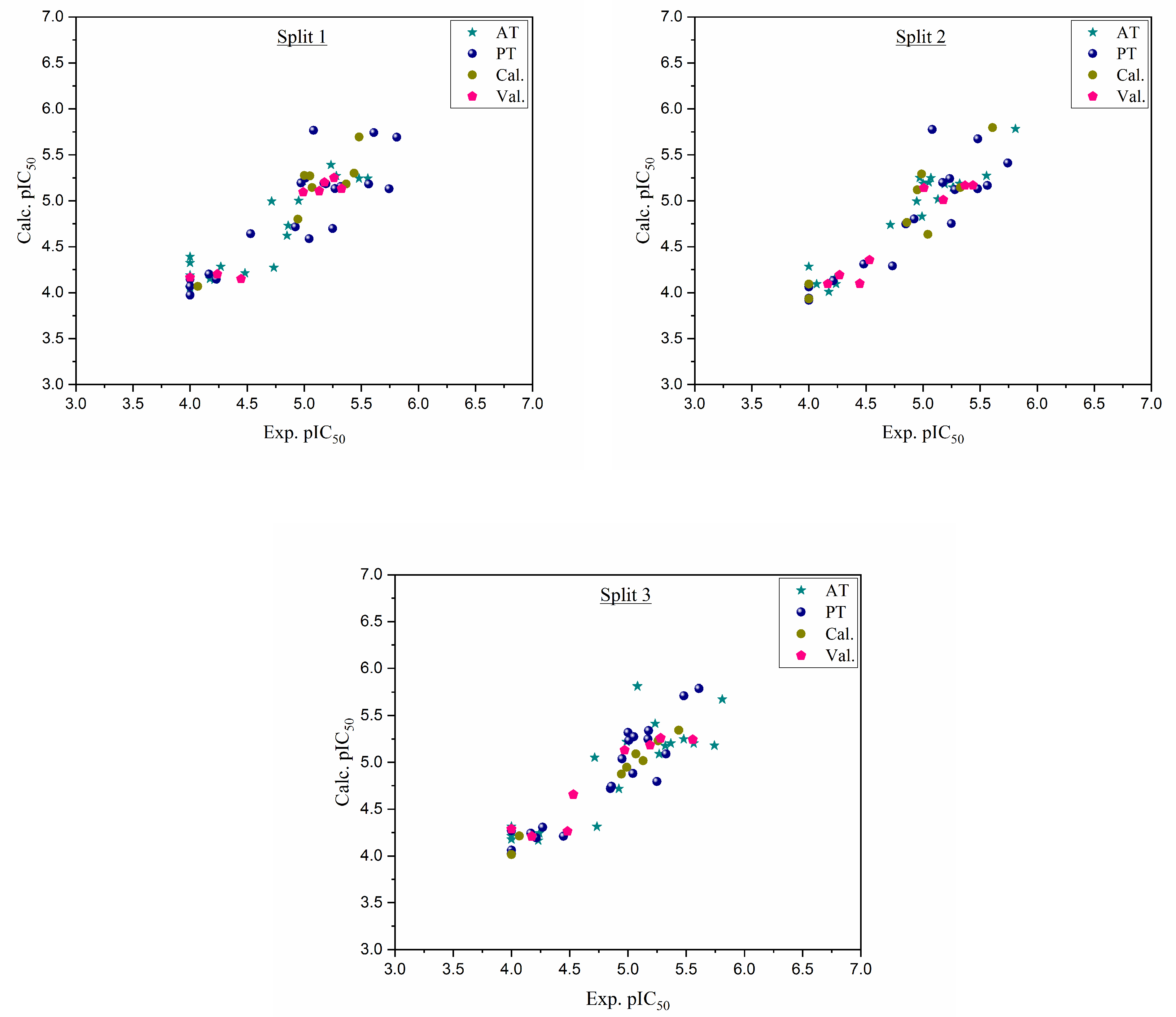
Funding

This research received no external funding.

Institutional Review Board Statement

Not applicable.

Informed Consent Statement

Not applicable.

Data Availability Statement

Data is contained within the article and Supplementary Material.

Acknowledgments

The authors would like to thank Paola Gramatica for providing a copy of the QSARINS Software.

Conflicts of Interest

The authors declare no conflict of interest.

References

  1. Oubahmane, M.; Hdoufane, I.; Bjij, I.; Lahcen, N.A.; Villemin, D.; Daoud, R.; Allali, A.E.; Cherqaoui, D. Host Cell Proteases Mediating SARS-CoV-2 Entry: An Overview. Curr. Top. Med. Chem. 2022, 22, 1776–1792. [Google Scholar] [CrossRef]
  2. Wang, P.; Nair, M.S.; Liu, L.; Iketani, S.; Luo, Y.; Guo, Y.; Wang, M.; Yu, J.; Zhang, B.; Kwong, P.D.; et al. Antibody resistance of SARS-CoV-2 variants B.1.351 and B.1.1.7. Nature 2021, 593, 130–135. [Google Scholar] [CrossRef] [PubMed]
  3. Bian, L.; Gao, F.; Zhang, J.; He, Q.; Mao, Q.; Xu, M.; Liang, Z. Effects of SARS-CoV-2 variants on vaccine efficacy and response strategies. Expert Rev. Vaccines 2021, 20, 365–373. [Google Scholar] [CrossRef] [PubMed]
  4. Subbarao, K. The success of SARS-CoV-2 vaccines and challenges ahead. Cell Host Microbe 2021, 29, 1111–1123. [Google Scholar] [CrossRef]
  5. Tao, K.; Tzou, P.L.; Nouhin, J.; Gupta, R.K.; de Oliveira, T.; Kosakovsky Pond, S.L.; Fera, D.; Shafer, R.W. The biological and clinical significance of emerging SARS-CoV-2 variants. Nat. Rev. Genet. 2021, 22, 757–773. [Google Scholar] [CrossRef] [PubMed]
  6. Citarella, A.; Scala, A.; Piperno, A.; Micale, N. SARS-CoV-2 Mpro: A Potential Target for Peptidomimetics and Small-Molecule Inhibitors. Biomolecules 2021, 11, 607. [Google Scholar] [CrossRef]
  7. Zhao, Y.; Zhu, Y.; Liu, X.; Jin, Z.; Duan, Y.; Zhang, Q.; Wu, C.; Feng, L.; Du, X.; Zhao, J.; et al. Structural basis for replicase polyprotein cleavage and substrate specificity of main protease from SARS-CoV-2. Proc. Natl. Acad. Sci. USA 2022, 119, e2117142119. [Google Scholar] [CrossRef]
  8. Tan, B.; Joyce, R.; Tan, H.; Hu, Y.; Wang, J. SARS-CoV-2 Main Protease Drug Design, Assay Development, and Drug Resistance Studies. Acc. Chem. Res. 2023, 56, 157–168. [Google Scholar] [CrossRef]
  9. Ullrich, S.; Ekanayake, K.B.; Otting, G.; Nitsche, C. Main protease mutants of SARS-CoV-2 variants remain susceptible to nirmatrelvir. Bioorg. Med. Chem. Lett. 2022, 62, 128629. [Google Scholar] [CrossRef]
  10. Zhang, L.; Lin, D.; Kusov, Y.; Nian, Y.; Ma, Q.; Wang, J.; von Brunn, A.; Leyssen, P.; Lanko, K.; Neyts, J.; et al. α-Ketoamides as Broad-Spectrum Inhibitors of Coronavirus and Enterovirus Replication: Structure-Based Design, Synthesis, and Activity Assessment. J. Med. Chem. 2020, 63, 4562–4578. [Google Scholar] [CrossRef]
  11. Zhang, L.; Lin, D.; Sun, X.; Curth, U.; Drosten, C.; Sauerhering, L.; Becker, S.; Rox, K.; Hilgenfeld, R. Crystal structure of SARS-CoV-2 main protease provides a basis for design of improved α-ketoamide inhibitors. Science 2020, 368, 409–412. [Google Scholar] [CrossRef] [PubMed]
  12. Silvestrini, L.; Belhaj, N.; Comez, L.; Gerelli, Y.; Lauria, A.; Libera, V.; Mariani, P.; Marzullo, P.; Ortore, M.G.; Palumbo Piccionello, A.; et al. The dimer-monomer equilibrium of SARS-CoV-2 main protease is affected by small molecule inhibitors. Sci. Rep. 2021, 11, 9283. [Google Scholar] [CrossRef] [PubMed]
  13. Goyal, B.; Goyal, D. Targeting the Dimerization of the Main Protease of Coronaviruses: A Potential Broad-Spectrum Therapeutic Strategy. ACS Comb. Sci. 2020, 22, 297–305. [Google Scholar] [CrossRef]
  14. Oubahmane, M.; Hdoufane, I.; Bjij, I.; Jerves, C.; Villemin, D.; Cherqaoui, D. COVID-19: In silico identification of potent α-ketoamide inhibitors targeting the main protease of the SARS-CoV-2. J. Mol. Struct. 2021, 1244, 130897. [Google Scholar] [CrossRef]
  15. Golbraikh, A.; Tropsha, A. Beware of q2! J. Mol. Graph. Model. 2002, 20, 269–276. [Google Scholar] [CrossRef]
  16. Ojha, P.K.; Mitra, I.; Das, R.N.; Roy, K. Further exploring rm2 metrics for validation of QSPR models. Chemom. Intell. Lab. Syst. 2011, 107, 194–205. [Google Scholar] [CrossRef]
  17. Zhang, J.-W.; Xiong, Y.; Wang, F.; Zhang, F.-M.; Yang, X.; Lin, G.-Q.; Tian, P.; Ge, G.; Gao, D. Discovery of 9,10-dihydrophenanthrene derivatives as SARS-CoV-2 3CLpro inhibitors for treating COVID-19. Eur. J. Med. Chem. 2022, 228, 114030. [Google Scholar] [CrossRef] [PubMed]
  18. Frisch, M.J.; Trucks, G.W.; Schlegel, H.B.; Scuseria, G.E.; Robb, M.A.; Cheeseman, J.R.; Scalmani, G.; Barone, V.; Mennucci, B.; Petersson, G.A.; et al. Gaussian 09. Wallingford C.T. 2009. Available online: http://gaussian.com/ (accessed on 10 March 2023).
  19. Mauri, A.; Bertola, M. Alvascience: A New Software Suite for the QSAR Workflow Applied to the Blood–Brain Barrier Permeability. Int. J. Mol. Sci. 2022, 23, 12882. [Google Scholar] [CrossRef] [PubMed]
  20. CORAL/Free Software for QSAR and NanoQSAR. Available online: http://www.insilico.eu/coral/ (accessed on 31 January 2023).
  21. Toropova, A.P.; Toropov, A.A. QSPR and nano-QSPR: What is the difference? J. Mol. Struct. 2019, 1182, 141–149. [Google Scholar] [CrossRef]
  22. Kumar, P.; Kumar, A. CORAL: QSAR models of CB1 cannabinoid receptor inhibitors based on local and global SMILES attributes with the index of ideality of correlation and the correlation contradiction index. Chemom. Intell. Lab. Syst. 2020, 200, 103982. [Google Scholar] [CrossRef]
  23. Liman, W.; Oubahmane, M.; Hdoufane, I.; Bjij, I.; Villemin, D.; Daoud, R.; Cherqaoui, D.; El Allali, A. Monte Carlo Method and GA-MLR-Based QSAR Modeling of NS5A Inhibitors against the Hepatitis C Virus. Molecules 2022, 27, 2729. [Google Scholar] [CrossRef] [PubMed]
  24. Duhan, M.; Sindhu, J.; Kumar, P.; Devi, M.; Singh, R.; Kumar, R.; Lal, S.; Kumar, A.; Kumar, S.; Hussain, K. Quantitative structure activity relationship studies of novel hydrazone derivatives as α-amylase inhibitors with index of ideality of correlation. J. Biomol. Struct. Dyn. 2022, 40, 4933–4953. [Google Scholar] [CrossRef] [PubMed]
  25. Toropova, A.P.; Toropov, A.A. The index of ideality of correlation: Improvement of models for toxicity to algae. Nat. Prod. Res. 2019, 33, 2200–2207. [Google Scholar] [CrossRef]
  26. IBM Corp. IBM SPSS Statistics for Windows; Version 28.0; Released 2021; IBM Corp: Armonk, NY, USA, 2021. [Google Scholar]
  27. Gramatica, P.; Chirico, N.; Papa, E.; Cassani, S.; Kovarich, S. QSARINS: A new software for the development, analysis, and validation of QSAR MLR models. J. Comput. Chem. 2013, 34, 2121–2132. [Google Scholar] [CrossRef]
  28. Gramatica, P.; Cassani, S.; Chirico, N. QSARINS-chem: Insubria datasets and new QSAR/QSPR models for environmental pollutants in QSARINS. J. Comput. Chem. 2014, 35, 1036–1044. [Google Scholar] [CrossRef] [PubMed]
  29. Gramatica, P. Principles of QSAR models validation: Internal and external. QSAR Comb. Sci. 2007, 26, 694–701. [Google Scholar] [CrossRef]
  30. Hdoufane, I.; Bjij, I.; Oubahmane, M.; Soliman, M.E.S.; Villemin, D.; Cherqaoui, D. In silico design and analysis of NS4B inhibitors against hepatitis C virus. J. Biomol. Struct. Dyn. 2022, 40, 1915–1929. [Google Scholar] [CrossRef]
  31. Hdoufane, I.; Ounaissi, D.; Dermoune, A.; Cherqaoui, D. Development of QSAR Models Using Singular Value Decomposition Method: A Case Study for Predicting Anti-HIV-1 and Anti-HCV Biological Activities. Biointerface Res. Appl. Chem. 2021, 12, 3090–3105. [Google Scholar] [CrossRef]
  32. OECD. Guidance Document on the Validation of (Quantitative) Structure—Activity Relationship [(Q)SAR] Models; OECD Series on Testing and Assessment; OECD: Berlin, Mexico, 2014; ISBN 978-92-64-08544-2. [Google Scholar]
  33. Toropov, A.A.; Toropova, A.P.; Lombardo, A.; Roncaglioni, A.; Benfenati, E.; Gini, G. CORAL: Building up the model for bioconcentration factor and defining it’s applicability domain. Eur. J. Med. Chem. 2011, 46, 1400–1403. [Google Scholar] [CrossRef]
  34. Dimitrov, S.; Dimitrova, G.; Pavlov, T.; Dimitrova, N.; Patlewicz, G.; Niemela, J.; Mekenyan, O. A Stepwise Approach for Defining the Applicability Domain of SAR and QSAR Models. J. Chem. Inf. Model. 2005, 45, 839–849. [Google Scholar] [CrossRef]
  35. Su, H.; Yao, S.; Zhao, W.; Li, M.; Liu, J.; Shang, W.; Xie, H.; Ke, C.; Hu, H.; Gao, M.; et al. Anti-SARS-CoV-2 activities in vitro of Shuanghuanglian preparations and bioactive ingredients. Acta Pharmacol. Sin. 2020, 41, 1167–1177. [Google Scholar] [CrossRef] [PubMed]
  36. Ferreira, J.C.; Fadl, S.; Rabeh, W.M. Key dimer interface residues impact the catalytic activity of 3CLpro, the main protease of SARS-CoV-2. J. Biol. Chem. 2022, 298, 102023. [Google Scholar] [CrossRef]
  37. Jiménez-Avalos, G.; Vargas-Ruiz, A.P.; Delgado-Pease, N.E.; Olivos-Ramirez, G.E.; Sheen, P.; Fernández-Díaz, M.; Quiliano, M.; Zimic, M.; COVID-19 Working Group in Perú; Agurto-Arteaga, A.; et al. Comprehensive virtual screening of 4.8 k flavonoids reveals novel insights into allosteric inhibition of SARS-CoV-2 MPRO. Sci. Rep. 2021, 11, 15452. [Google Scholar] [CrossRef] [PubMed]
  38. Discovery Studio Visualizer 3.0. Available online: https://discover.3ds.com/discovery-studio-visualizer-download (accessed on 20 September 2022).
  39. The PyMOL Molecular Graphics System; Version 1.8; Shrodinger LLC: New York, NY, USA, 2015.
  40. Van Der Spoel, D.; Lindahl, E.; Hess, B.; Groenhof, G.; Mark, A.E.; Berendsen, H.J.C. GROMACS: Fast, flexible, and free. J. Comput. Chem. 2005, 26, 1701–1718. [Google Scholar] [CrossRef]
  41. Abraham, M.J.; Murtola, T.; Schulz, R.; Páll, S.; Smith, J.C.; Hess, B.; Lindahl, E. GROMACS: High performance molecular simulations through multi-level parallelism from laptops to supercomputers. SoftwareX 2015, 1–2, 19–25. [Google Scholar] [CrossRef]
  42. Jo, S.; Kim, T.; Iyer, V.G.; Im, W. CHARMM-GUI: A web-based graphical user interface for CHARMM. J. Comput. Chem. 2008, 29, 1859–1865. [Google Scholar] [CrossRef] [PubMed]
  43. Lee, J.; Cheng, X.; Swails, J.M.; Yeom, M.S.; Eastman, P.K.; Lemkul, J.A.; Wei, S.; Buckner, J.; Jeong, J.C.; Qi, Y.; et al. CHARMM-GUI Input Generator for NAMD, GROMACS, AMBER, OpenMM, and CHARMM/OpenMM Simulations Using the CHARMM36 Additive Force Field. J. Chem. Theory Comput. 2016, 12, 405–413. [Google Scholar] [CrossRef]
  44. Grace. Available online: https://plasma-gate.weizmann.ac.il/Grace/ (accessed on 5 September 2022).
  45. Valdés-Tresanco, M.S.; Valdés-Tresanco, M.E.; Valiente, P.A.; Moreno, E. gmx_MMPBSA: A New Tool to Perform End-State Free Energy Calculations with GROMACS. J. Chem. Theory Comput. 2021, 17, 6281–6291. [Google Scholar] [CrossRef]
  46. Pires, D.E.V.; Blundell, T.L.; Ascher, D.B. pkCSM: Predicting Small-Molecule Pharmacokinetic and Toxicity Properties Using Graph-Based Signatures. J. Med. Chem. 2015, 58, 4066–4072. [Google Scholar] [CrossRef]
  47. Molecular Properties Prediction-Osiris Property Explorer. Available online: https://www.organic-chemistry.org/prog/peo/ (accessed on 3 January 2023).
Figure 1. Graphical representation of experimental pIC50 versus calculated pIC50 for three splits.
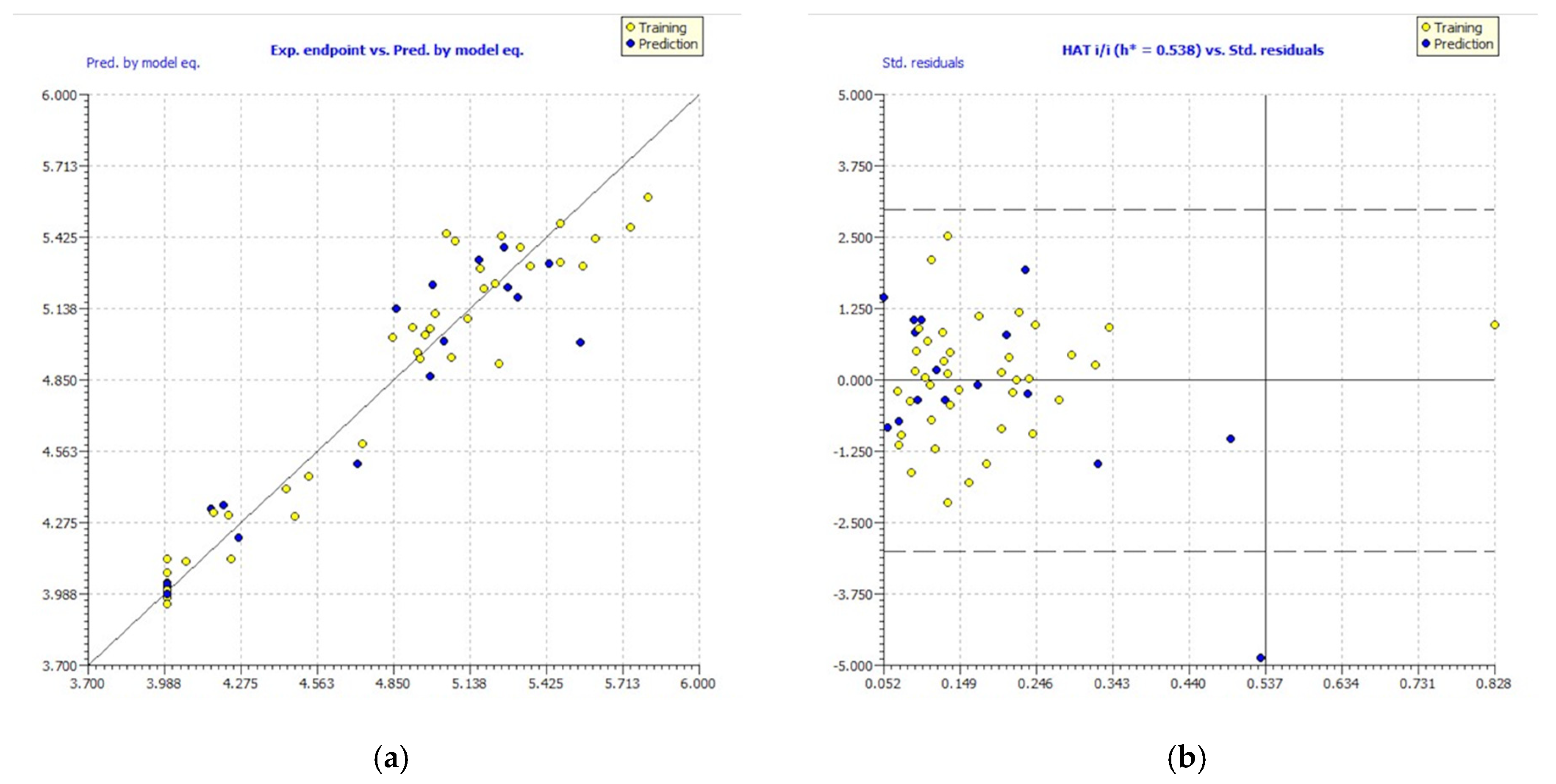
Pharmaceuticals 16 00608 g001
Figure 2. Experimental vs. predicted pIC50 values computed by GA-MLR (a). William’s plot (b).
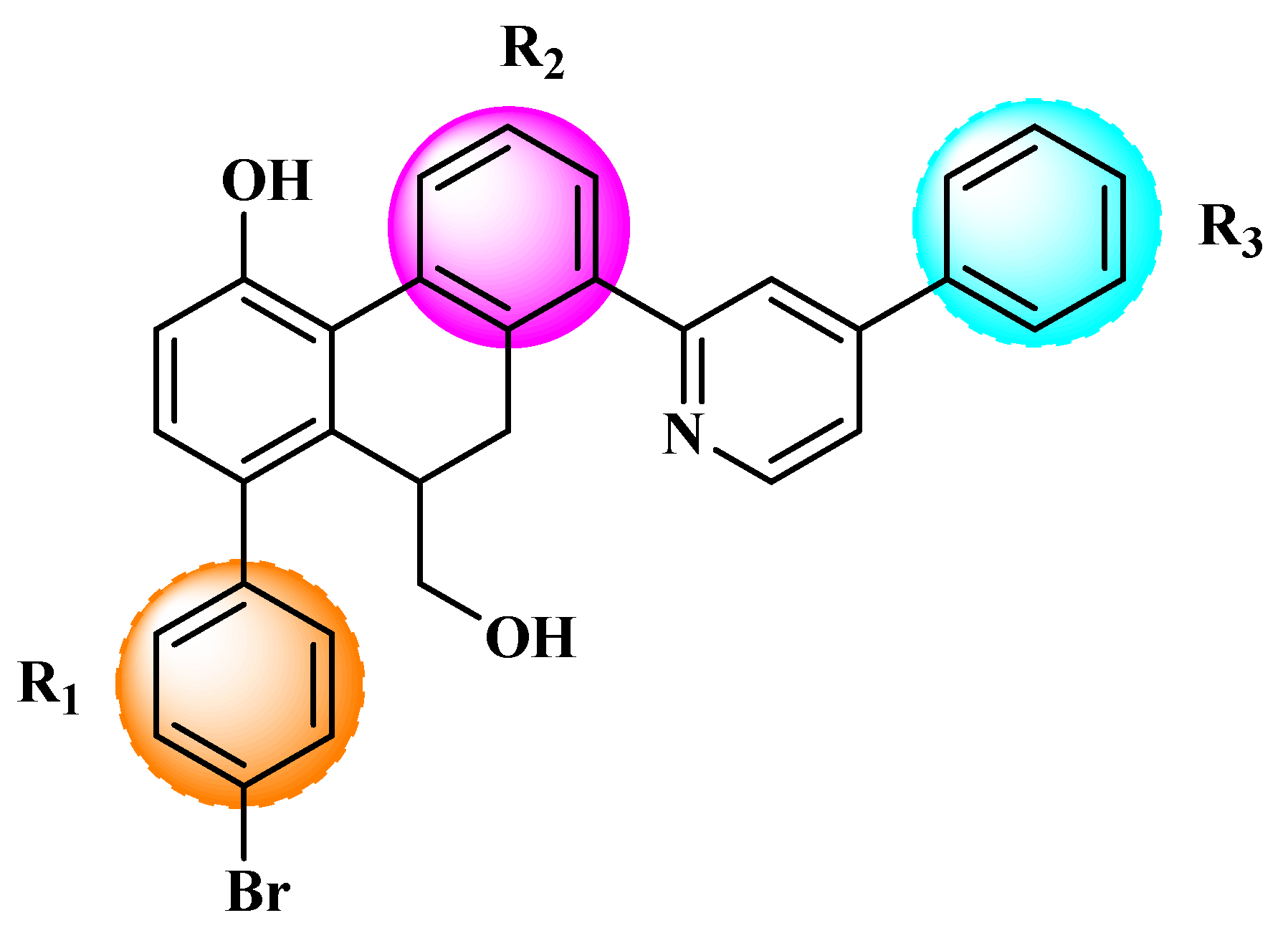
Pharmaceuticals 16 00608 g002
Figure 3. Chemical structures of the newly designed compounds.
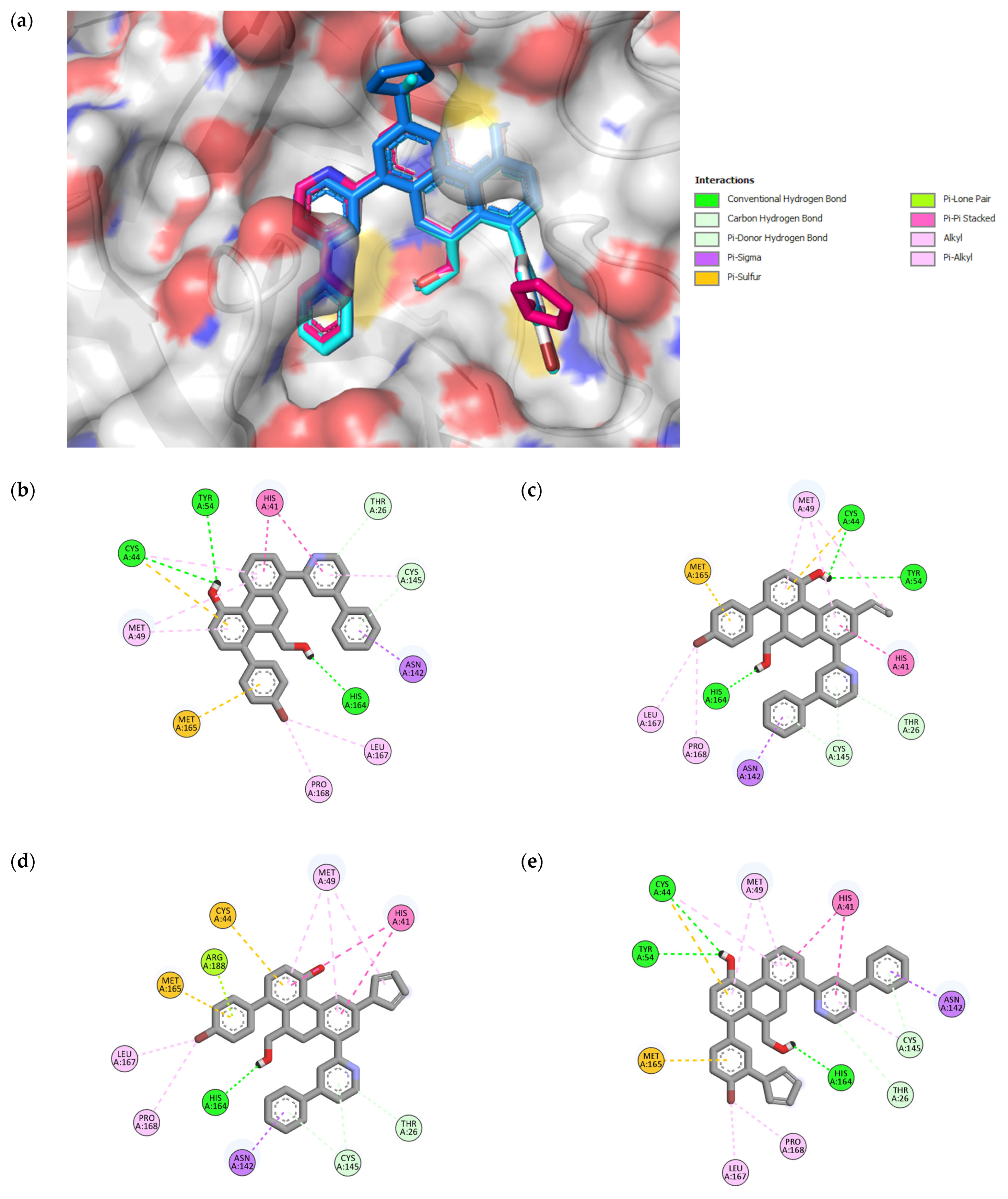
Pharmaceuticals 16 00608 g003
Figure 4. 3D representation of superimposition of the binding poses within the CS of SARS-CoV-2 Mpro of 49, 49n, 49p, and 49x molecules in white, cyan, magenta and blue color respectively (a); 2D representation of interactions within the CS of SARS-CoV-2 Mpro of 49 (b), 49n (c), 49p (d), and 49x (e) molecules.
Pharmaceuticals 16 00608 g004
Figure 5. 3D representation of superimposition of the binding poses within the DIS of SARS-CoV-2 of 49, 49n, 49p, and 49x molecules in white, cyan, magenta and blue color respectively (a); 2D representation of interactions within the DIS of SARS-CoV-2 Mpro of 49 (b), 49n (c), 49p (d), and 49x (e) molecules.
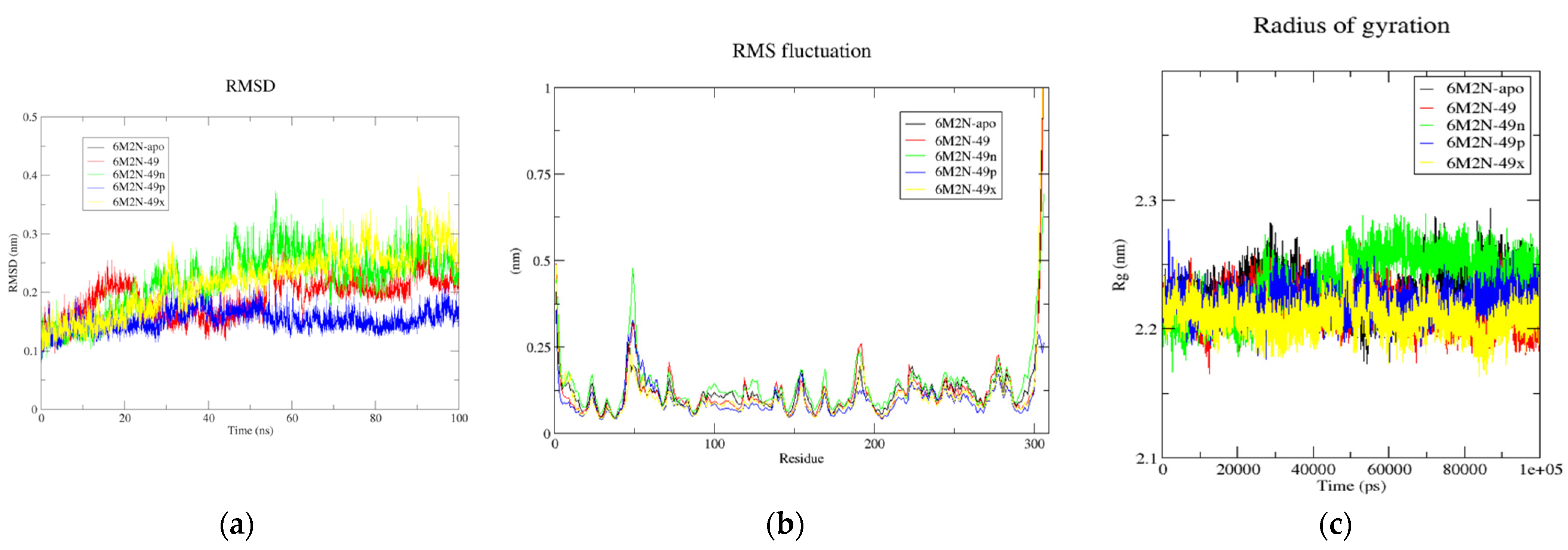
Pharmaceuticals 16 00608 g005
Figure 6. (a) Time-dependent RMSD of c-α backbone of the Mpro-apo, 6M2N-49, 6M2N-49n, 6M2N-49p, and 6M2N-49x. (b) The RMSF for c-α atoms of Mpro-apo, 6M2N-49, 6M2N-49n, 6M2N-49p, and 6M2N-49x. (c) Plot of Rg vs. time for Mpro-apo, 6M2N-49, 6M2N-49n, 6M2N-49p, and 6M2N-49x.
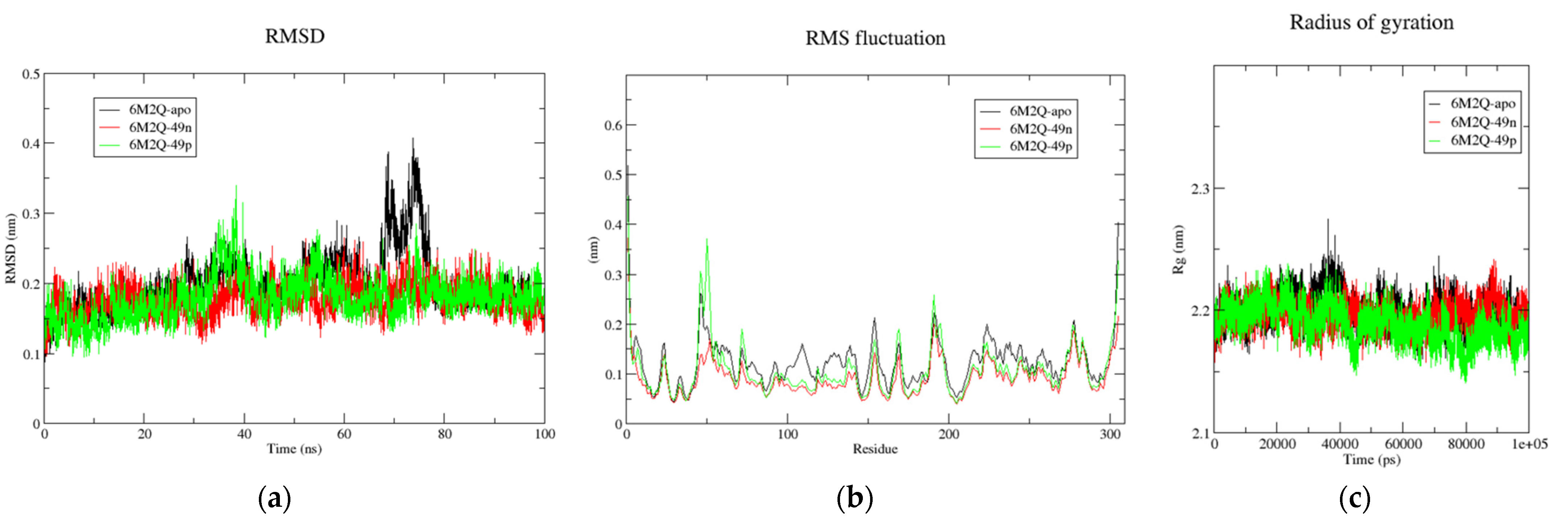
Pharmaceuticals 16 00608 g006
Figure 7. (a) Time-dependent RMSD of c-α backbone of the Mpro-apo, 6M2N-49n, and 6M2N-49p. (b) The RMSF for c-α atoms of Mpro-apo, 6M2N-49n, and 6M2N-49p. (c) Plot of Rg vs. time for Mpro-apo, 6M2N-49n, and 6M2N-49p.
Pharmaceuticals 16 00608 g007
Table 1. Statistical parameters of built QSAR models and their corresponding equations.
SplitTFSetnR2CCCIICQ2Q2F1Q2F2Q2F3Rm2avΔRm2Crp2Equation
1TF1AT190.80310.89080.65180.7605 0.7855pIC50 = 1.8172593 (+− 0.0736101) + 0.0553060 (+− 0.0014479) × DCW(1,1)
PT200.72370.81520.41760.6364 0.6964
Cal80.80850.89650.74680.52380.84680.78540.88540.72700.04380.7259
Val80.75790.84900.63720.5803 0.65450.1869
TF2AT190.81450.89780.81230.7734 0.7868pIC50 = 2.1090187 (+− 0.0660490) + 0.0635121 (+− 0.0016442) × DCW(5,14)
PT200.75100.86190.64010.6889 0.7309
Cal80.85360.91820.92390.66570.87430.82390.90600.78740.10080.7687
Val80.91610.95490.84330.8274 0.87710.0040
2TF1AT200.93140.96450.64340.9187 0.8879pIC50 = 2.0227798 (+− 0.0329913) + 0.0786046 (+− 0.0009506) × DCW(7,5)
PT190.88210.92450.42170.8428 0.8595
Cal80.80390.88570.61910.67880.73310.73290.75940.68300.18300.6787
Val80.85060.88260.47030.7229 0.78270.1187
TF2AT200.91910.95790.78440.9023 0.9029pIC50 = 1.7915330 (+− 0.0454500) + 0.0672532 (+− 0.0010114) × DCW(3,17)
PT190.82830.90010.75110.7652 0.8001
Cal80.86120.92510.92770.78450.83740.83730.85350.79320.12850.8266
Val80.92030.91570.67680.8508 0.88250.0647
3TF1AT190.74240.85210.77540.6545 0.7102pIC50 = 1.9879653 (+− 0.1287947) + 0.0650533 (+− 0.0030713) × DCW(3,1)
PT200.81290.89830.54420.7805 0.8008
Cal90.97360.97120.48880.96150.94920.94830.96220.86470.03790.9167
Val70.85890.90680.76340.7030 0.67790.1627
TF2AT190.74730.85540.77800.6645 0.6957pIC50 = 2.0784826 (+− 0.1186544) + 0.0690012 (+− 0.0031186) × DCW(10,7)
PT200.82100.90390.54960.7899 0.7929
Cal90.98600.98640.99250.97000.97580.97540.98200.88490.02410.8731
Val70.87280.91970.77400.7444 0.71690.1417
Table 2. Molecular descriptors and their description.
Molecular DescriptorDescription
Eig09_AEA(dm)Eigenvalue n. 9 from augmented edge adjacency matrix weighted by dipole moment
P_VSA_MR_5P_VSA-like on Molar Refractivity, bin 5
s3_numSharedNeighborsNumber of shared neighbours in substituent 3 with other substituents
s3_relPathLength_2Maximum path length of the substituent 3 normed by s3_size
SpMin2_Bh(m)Smallest eigenvalue n. 2 of Burden matrix weighted by mass
GATS5mGeary autocorrelation of lag 5 weighted by mass
Table 3. Promoters of increase and decrease of pIC50 endpoint value from split 2 and their description.
CWs Probe 1CWs Probe 2CWs Probe 3NAT aNPT bNCal cDefect [SAk] dComment
Promoters of increase
(...........0.212840.245910.24281201980.0000Branching
(...O...(...1.238891.327191.06767201980.0000Two-sided branching of oxygen
++++N---O===0.928381.332021.79720201980.0000Presence of nitrogen with oxygen
1...........0.302430.030650.22419201980.0000Presence of one ring
C...........0.017680.106100.24270201980.0000Presence of sp3 carbon
c...(.......0.101230.121920.30233201980.0000Sp2 carbon with branching
c...(...c...0.141090.278610.30707201980.0000Branching between two sp2 carbons
c...........0.577560.619850.68283201980.0000Presence of a sp2 carbon
c...2.......0.031990.017940.13095201980.0000Presence of at least two aromatic rings/Presence of sp2 carbon with two rings
c...2...c...0.640830.330250.27204201980.0000Aromatic ring surrounded by two sp2 carbons
c...c...(...0.457610.468210.64020201980.0000Presence of two sp2 carbons with branching
c...c.......0.094290.445190.11101201980.0000Presence of two sp2 carbons
c...c...c...0.289560.776330.66046201980.0000Presence of three sp2carbons
C...C...(...0.404710.849991.11520191980.0019Presence of two sp3 carbons with branching
Promoters of decrease
O...........−0.96058−1.30101−1.49847201980.0000Presence of oxygen
n........…−1.27893−1.65511−1.62009201980.0000Presence of sp2 nitrogen
n...c.......−0.11779−0.15247−0.22729201970.0046Presence of sp2 nitrogen with sp2 carbon
=……….−0.52134−0.04031−0.07066151970.0057Presence of double covalent bond
c...C.......−0.28402−0.70453−0.4430291240.0038Combination of sp2 carbon and sp3 carbon
c...(...C...−0.24438−0.23144−0.6365481240.0083Branching between sp2 carbon and sp3 carbon
C...O...C...−0.19900−0.49944−0.588117730.0025Sp3 oxygen surrounded by two sp3 carbons
NAT a, NPT b, and NCal c represent the number of SMILES (samples) in AT, PT, and Cal sets, respectively, that comprise a particular attribute (SAk). Defect [SAk] d is calculated as the difference between the probability of SAk in the training and calibration sets divided by the total number of SAk in the training and calibration sets.
Table 4. The newly designed compounds and their predicted pIC50 using the Monte Carlo optimization and the GA-MLR models.
Binding Affinity (Kcal/mol)
CompoundsChemical StructureCatalytic SiteDimer Interface Site
49 (ref)Pharmaceuticals 16 00608 i001−11.47−8.65
49nPharmaceuticals 16 00608 i002−12.63−9.18
49pPharmaceuticals 16 00608 i003−12.98−9.95
49xPharmaceuticals 16 00608 i004−12.85−9.06
Table 5. The calculated average parameters for all the systems throughout 100 ns MD simulation run.
Systems6M2N-Apo6M2N-496M2N-49n6M2N-49p6M2N-49x
RMSD (nm)0.2200.1910.2210.1520.241
RMSF (nm)0.1150.1130.1310.0920.103
Rg (nm)2.2232.2092.2312.2132.203
Table 6. Detailed binding free energy calculated by MM/GBSA for all complexes. All the values are given in kcal/mol.
Systems6M2N-496M2N-49n6M2N-49p6M2N-49x
ΔEvdw−31.98−33.54−40.95−51.68
ΔEele−11.93−8.38−16.3−18.1
ΔEGB31.126.4842.7645.97
ΔEsurf−4.26−4.19−5.28−6.5
ΔGgas−43.91−41.92−57.25−69.78
ΔGsolv26.8422.2937.4839.48
Δtotal−17.07−19.63−19.77−30.3
Table 7. The calculated average parameters for all the systems after 100 ns MD simulation run.
Systems6M2Q-Apo6M2Q-49n6M2Q-49p
RMSD (nm)0.1980.1760.178
RMSF (nm)0.1160.0870.102
Rg (nm)2.1942.1902.183
Table 8. ADMET properties for the designed compounds and the reference compound.
Compounds4949n49p49x
Pharmacokinetic and ADME properties
HIA (%)97.57597.49497.53497.873
BBB (Log BB)−0.428−0.249−0.214−0.218
P-glycoprotein substrateYesNoNoNo
CYP2C19 inhibitorNoNoNoNo
CYP2C9 inhibitorNoNoNoNo
CYP2D6 inhibitorNoNoNoNo
CYP3A4 inhibitorNoNoNoNo
Toxicological properties
MutagenicNo riskNo riskNo riskNo risk
TumorigenicNo riskNo riskNo riskNo risk
IrritantNo riskNo riskNo riskNo risk
Reproductive effectNo riskNo riskNo riskNo risk
Table 9. Percentage of the identity of the three splits.
Split 1 (%)Split 2 (%)Split 3 (%)
SetTotalATPTCalValTotalATPTCalValTotalATPTCalVal
Split 1 (%)10010010010010025.525.635.90.025.032.736.835.050.00.0
Split 2 (%) 10010010010010030.935.941.012.512.5
Split 3 (%) 100100100100100
Table 10. The detailed description of SMILES attributes.
SMILES AttributesDescription
SkOne symbol or two symbols that cannot be examined separately
SSkCombination of two SMILES-atomes
SSSkCombination of three SMILES-atomes
PAIRAlliance of two descriptors NOSP a and BOND b
HARDExistence of some chemical element
CmaxNumber of rings
OmaxNumber of oxygen atoms
NmaxNumber of nitrogen atoms
NOSP a descriptors are the structural features showing the presence or absence of nitrogen, oxygen, sulfur, phosphorus, while the BOND b descriptors respond to the presence or absence of double, triple, or stereochemical covalent bonds (=, #, @ or @@).
Table 11. List of key residues of SARS-CoV-2 Mpro.
Role in the SARS-CoV-2 MproResidues
Substrate bindingHIS41, MET49, GLY143, SER144, HIS163, HIS164, MET165, GLU166, LEU167, ASN187, ARG188, GLN189, THR190, ALA191, GLN192
DimerizationARG4, SER10, GLY11, GLU14, ASN28, SER139, PHE140, SER147, GLU290, ARG298
Catalytic dyadHIS41, CYS145
Disclaimer/Publisher’s Note: The statements, opinions and data contained in all publications are solely those of the individual author(s) and contributor(s) and not of MDPI and/or the editor(s). MDPI and/or the editor(s) disclaim responsibility for any injury to people or property resulting from any ideas, methods, instructions or products referred to in the content.

