

Neustrelitz Total Electron Content Model for Galileo Performance: A Position Domain Analysis


Abstract
:1. Introduction
2. Absolute Positioning Computation and Ionospheric Models
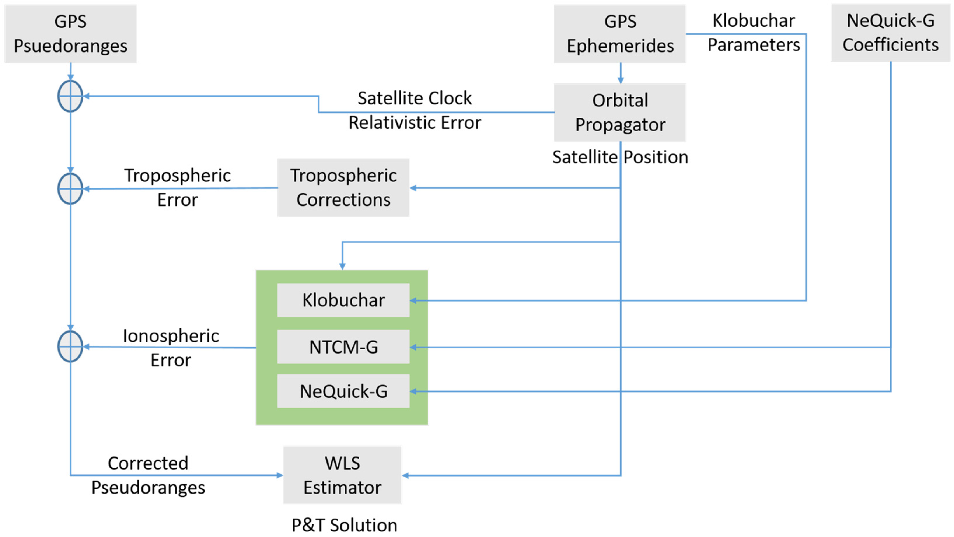
2.1. Absolute Positioning
2.2. Ionosperic Models
2.2.1. Klobuchar
2.2.2. NeQuick-G
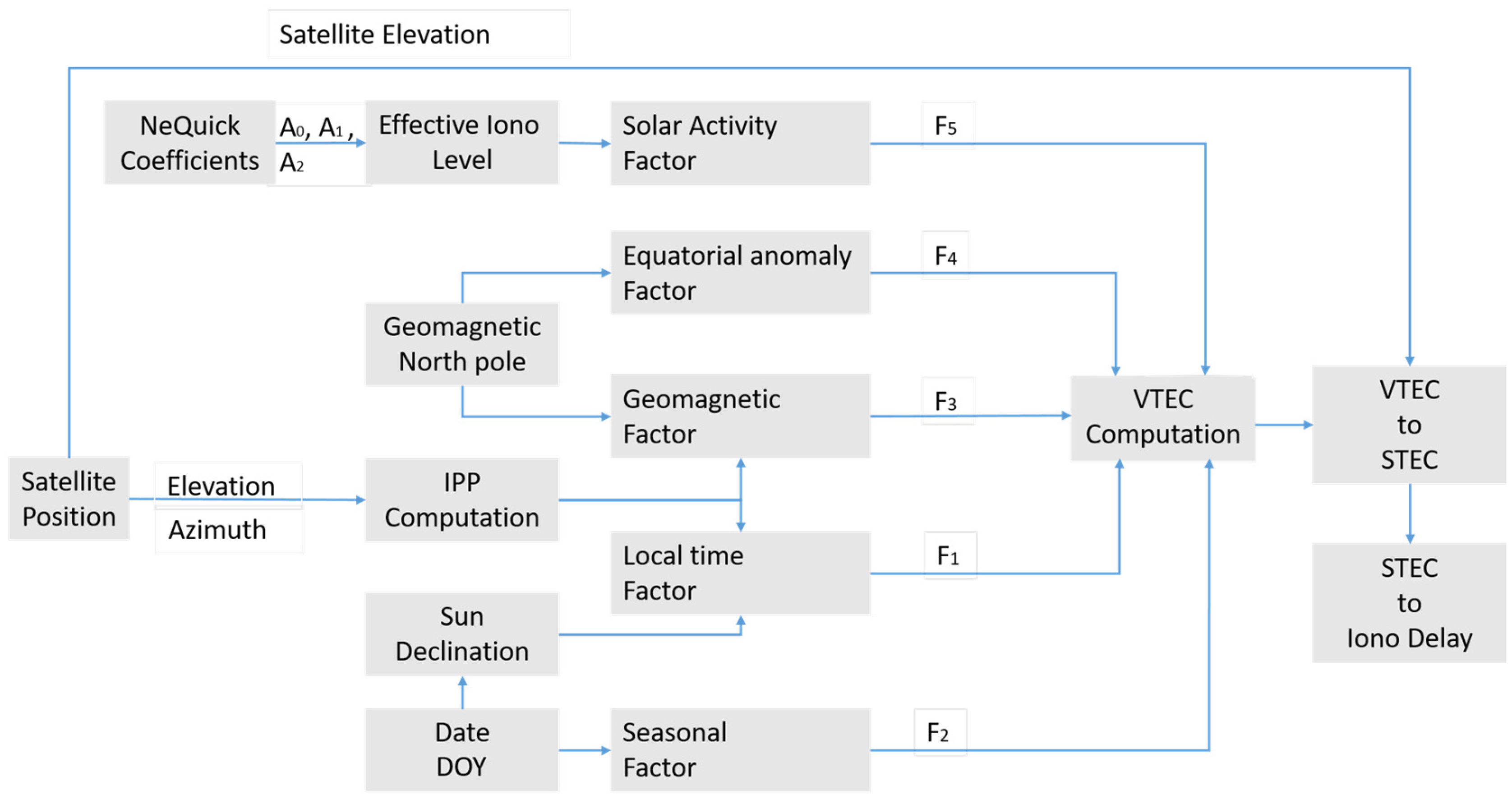
2.2.3. NTCM-G
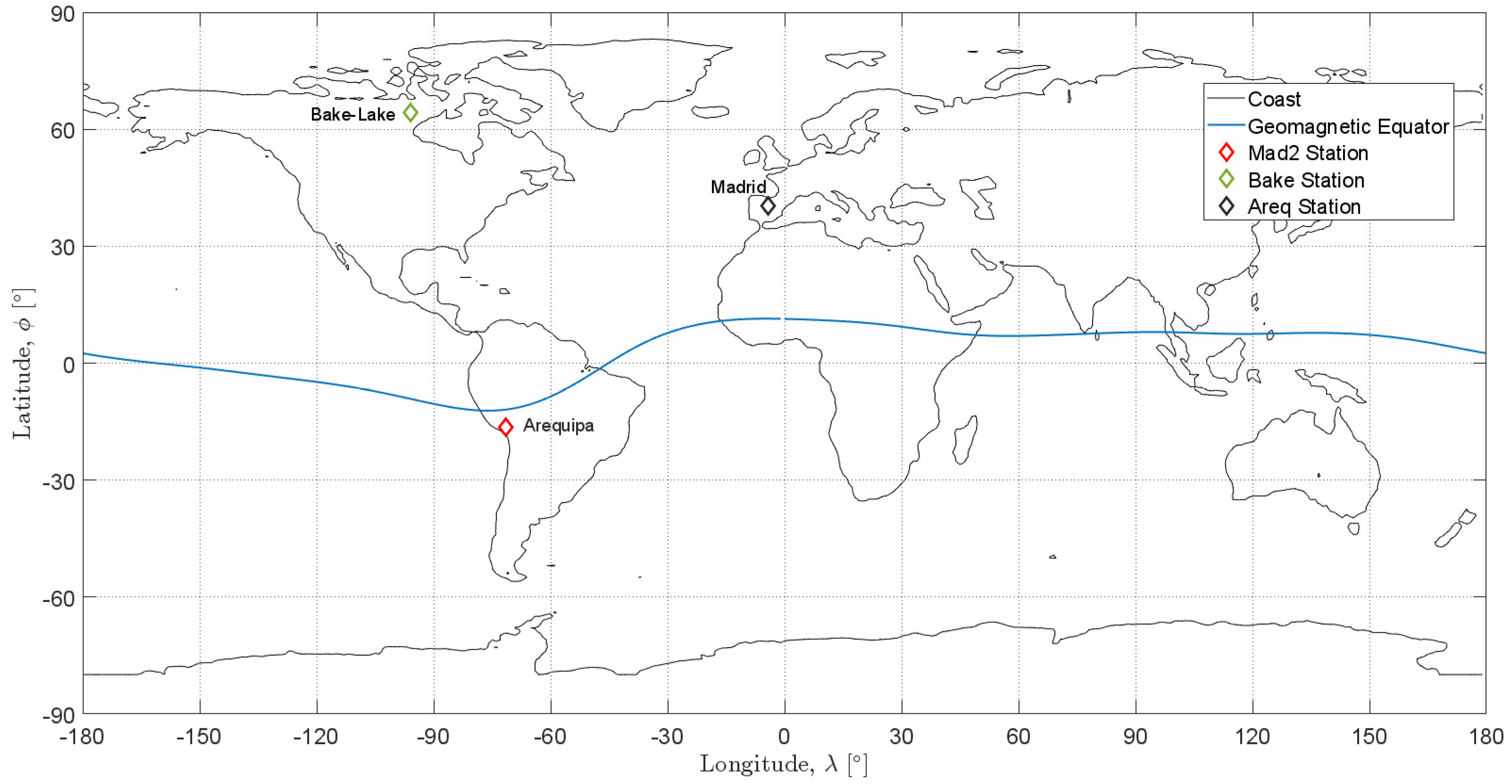
3. Experimental Setup
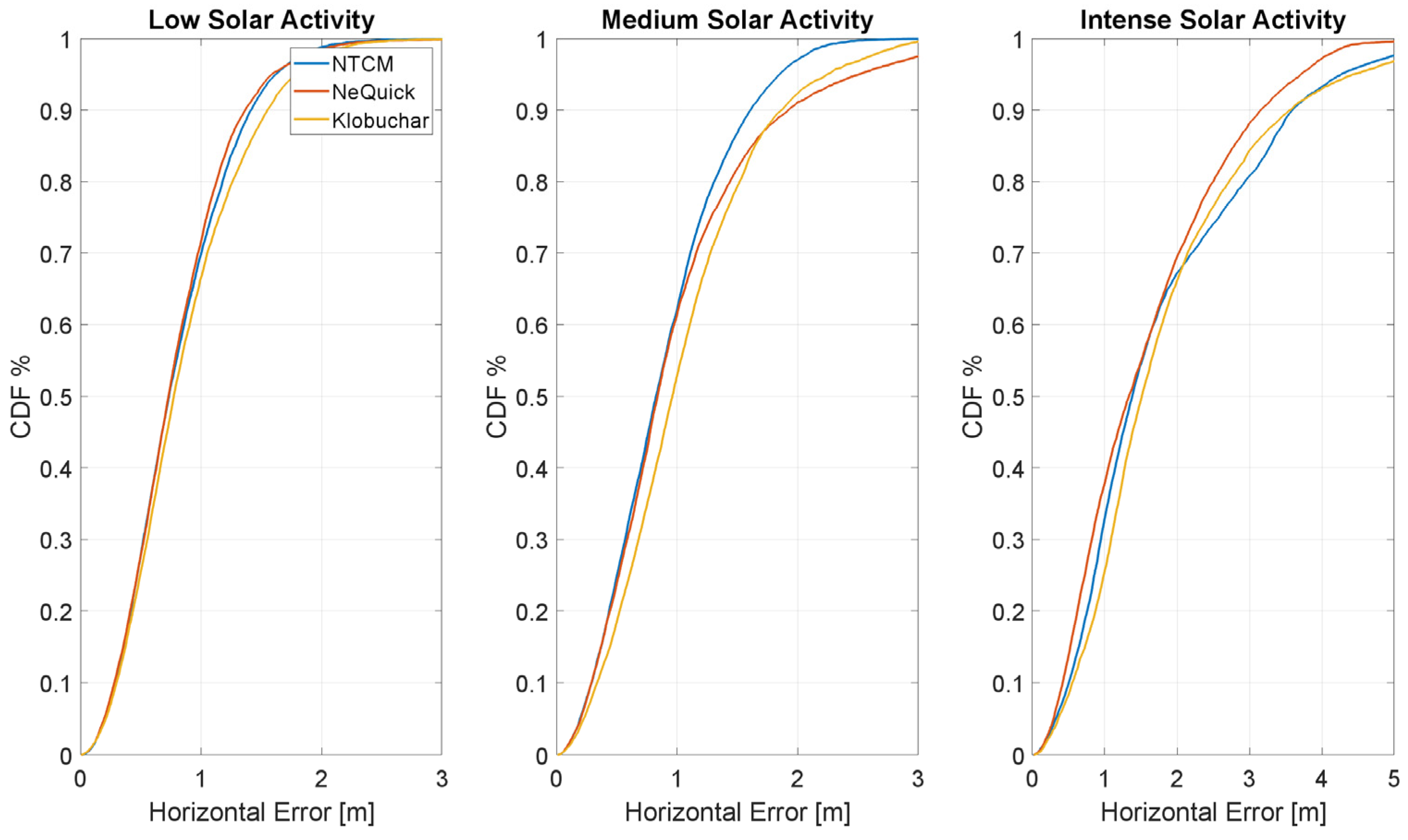
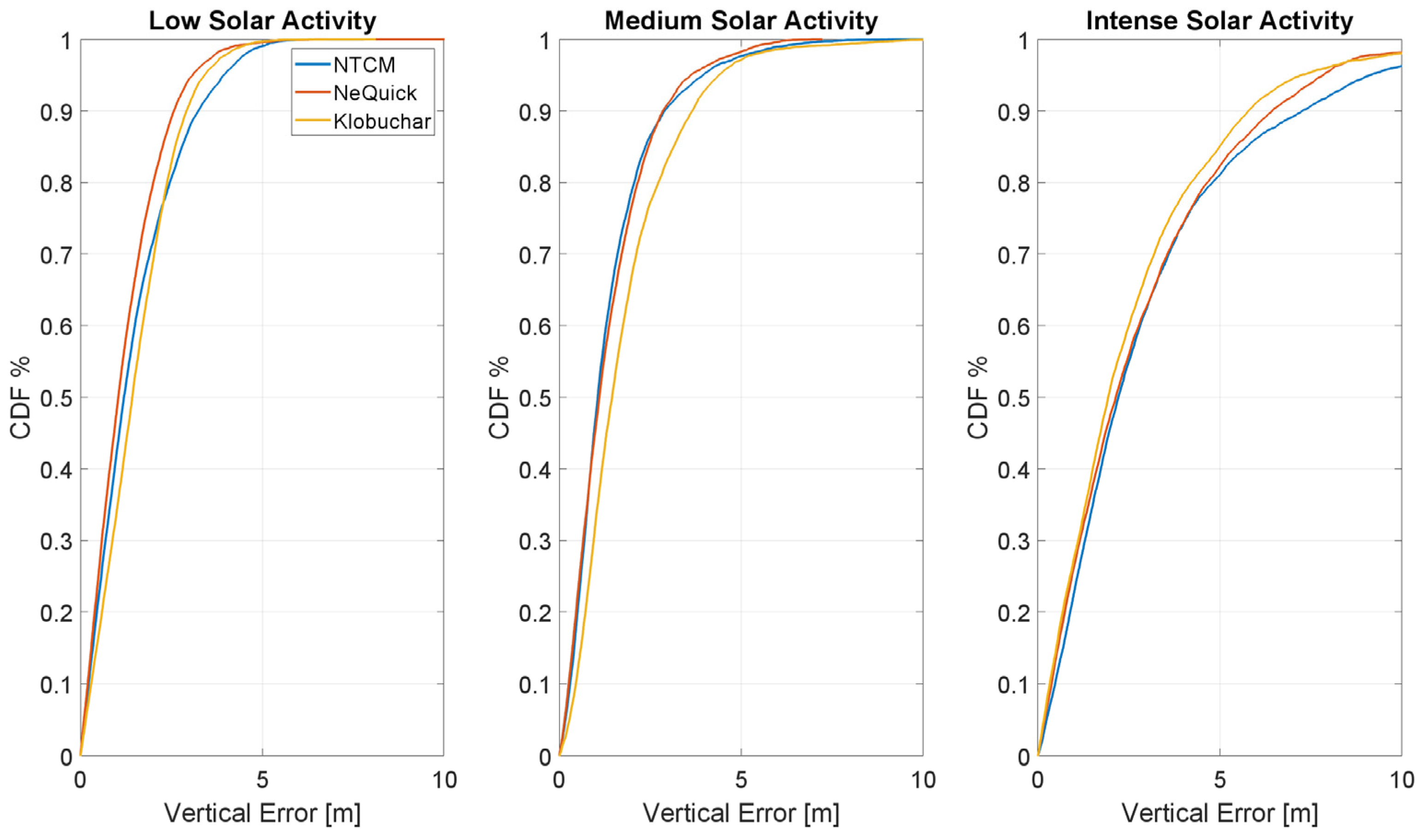
4. Results
- -
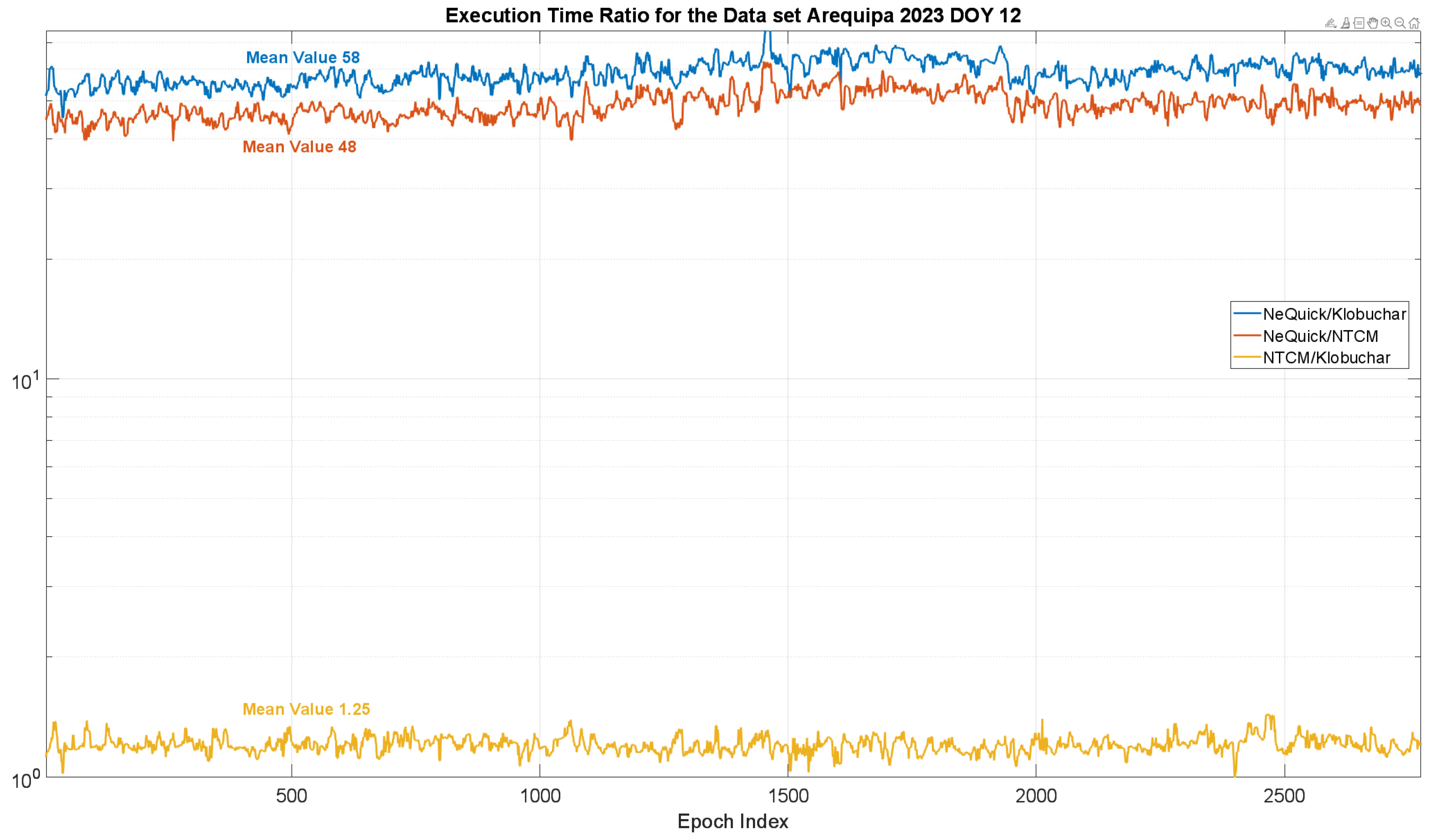
- Execution time, defined as the time needed to compute the ionospheric corrections;
- -
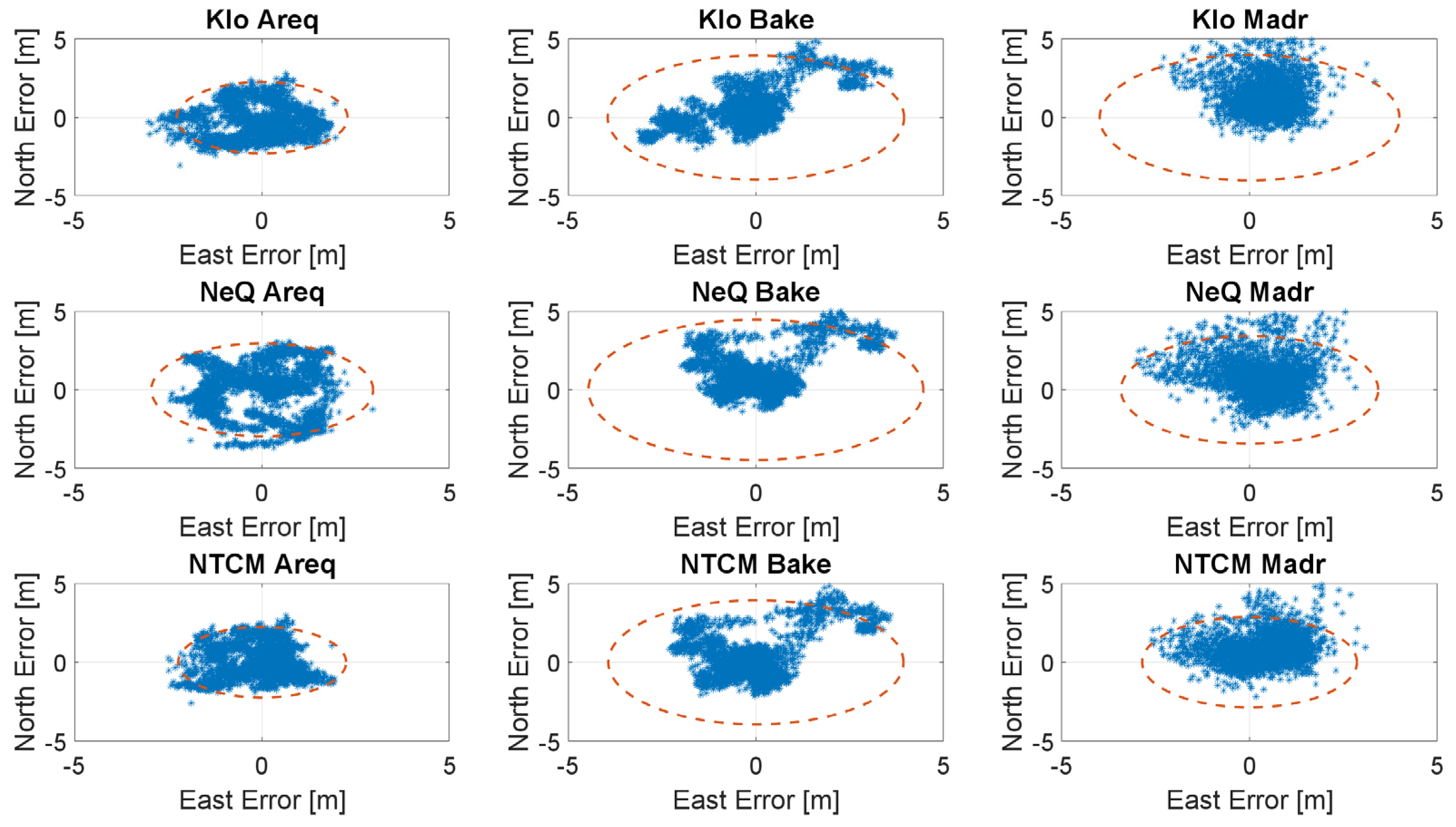
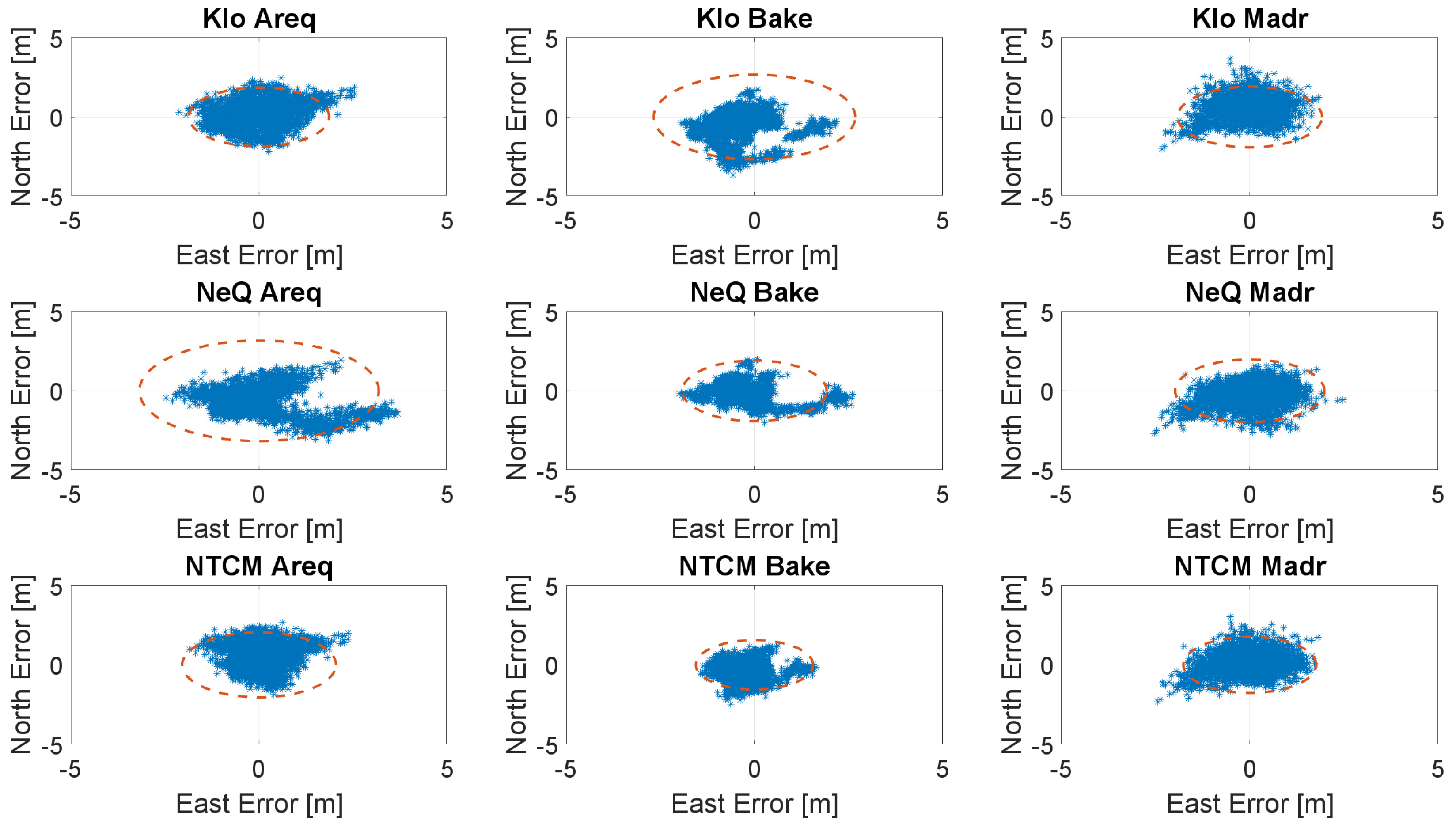
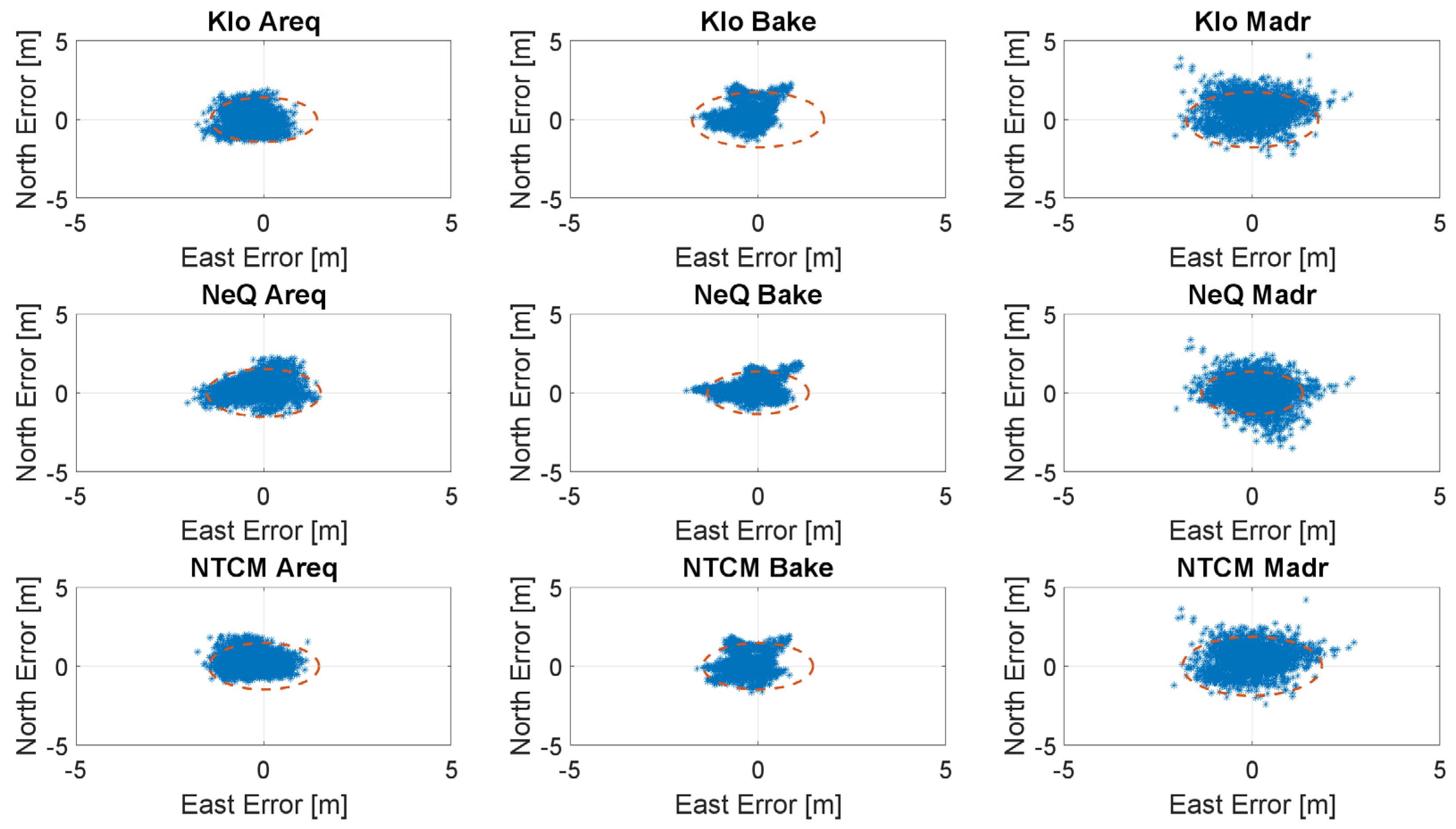
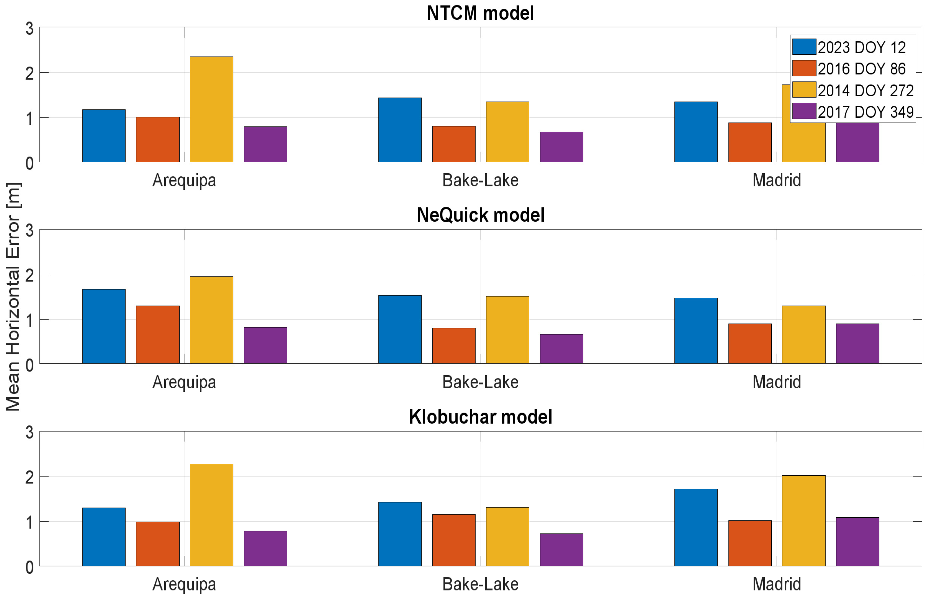
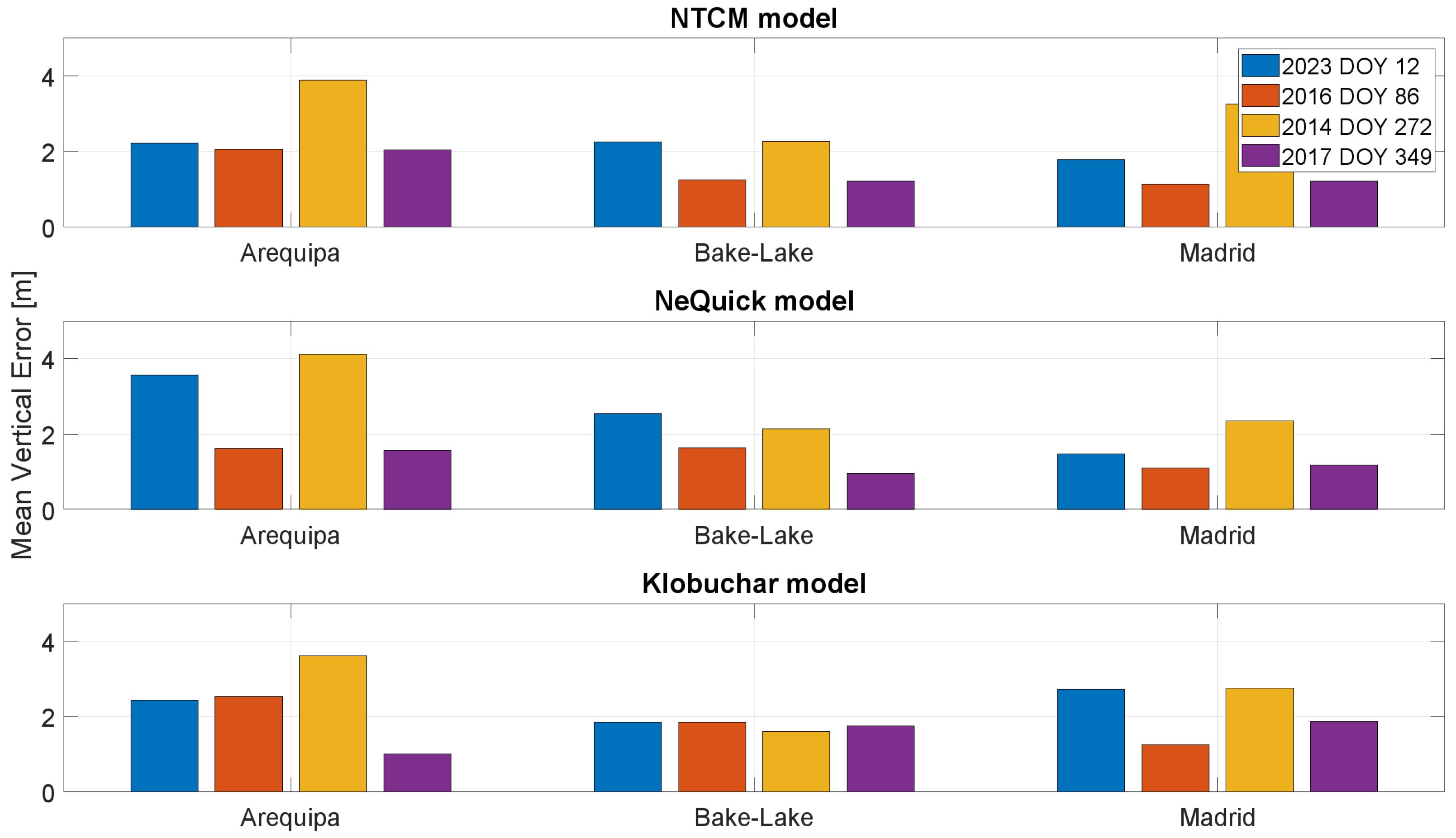
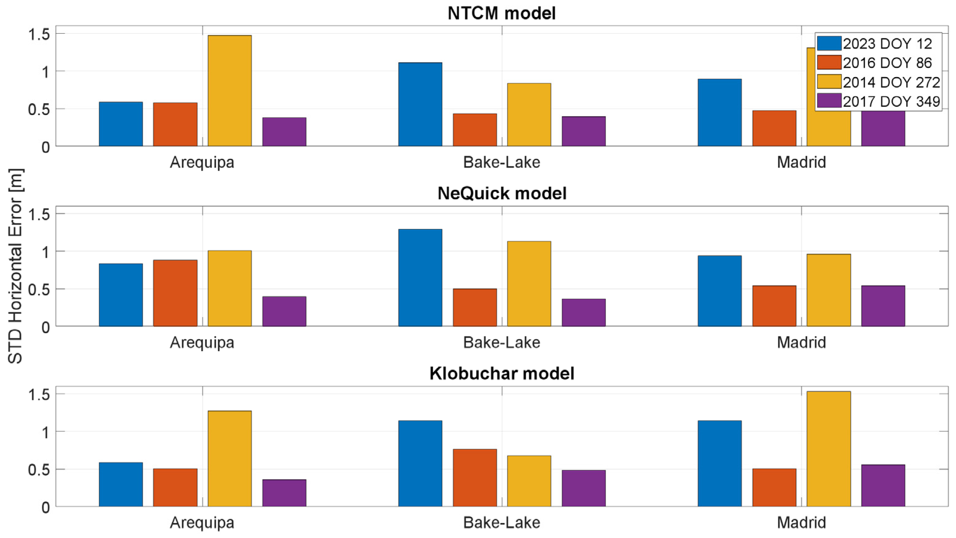
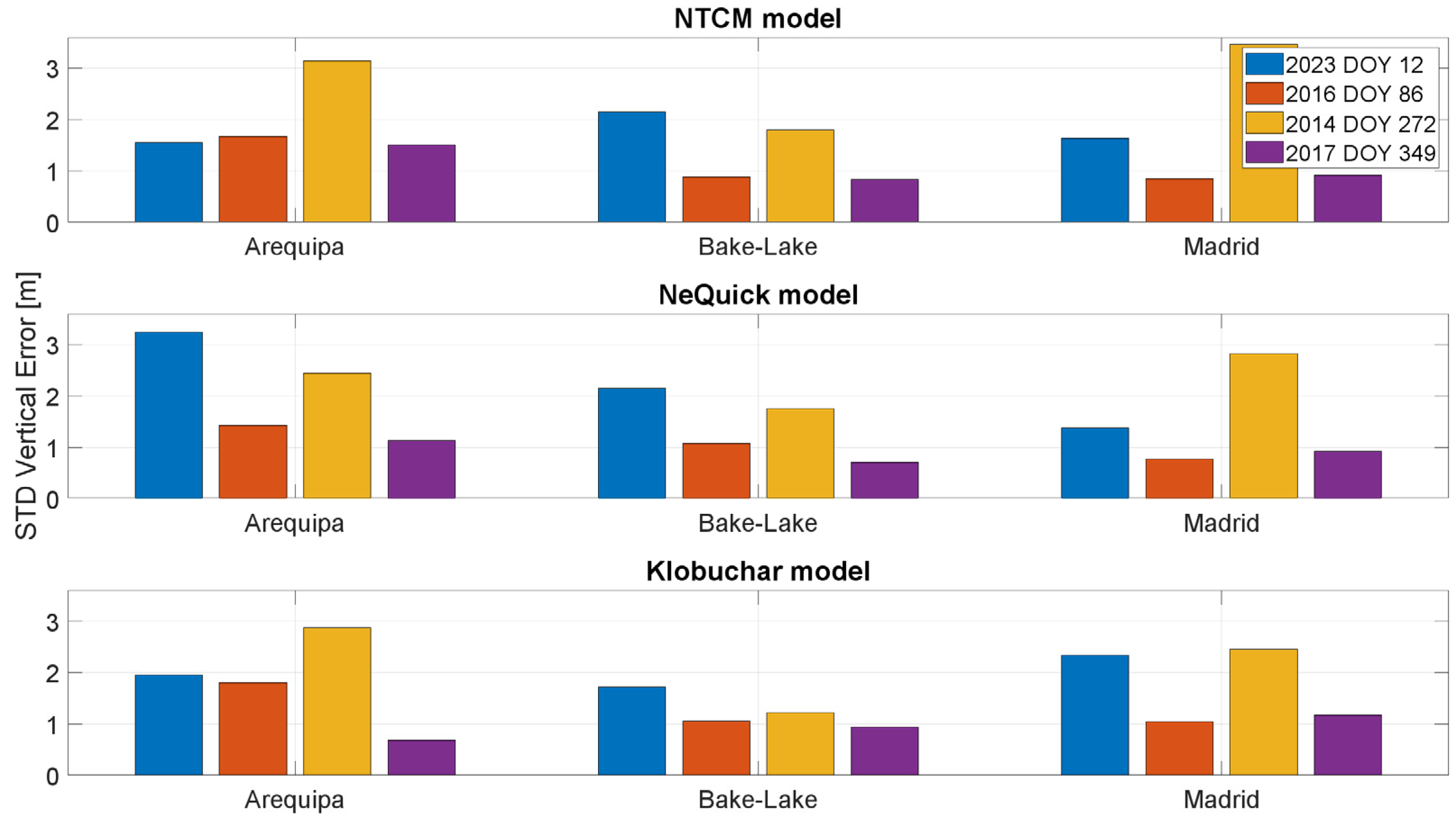
- Position error, computed as the difference between the estimated position solution and the reference coordinates of the station. The parameters used to evaluate the performance are the mean, standard deviation and 95th percentile of horizontal and vertical errors.
- -
- the upper boxes concern the results obtained using the Klobuchar model;
- -
- the central boxes concern results obtained using NeQuick-G;
- -
- the lower boxes concern results obtained using the NTCM-G model.
5. Conclusions
Author Contributions
Funding
Institutional Review Board Statement
Informed Consent Statement
Data Availability Statement
Acknowledgments
Conflicts of Interest
References
- Bassiri, J.; Hajj, G. Modeling the GPS Signal Propagation Through the Ionosphere; National Aeronautics and Space Administration: Washington, DC, USA, 1992.
- Hoffmann-Wellenhof, B.; Lichtenegger, H.; Collins, J. Global Positioning System: Theory and Practice, 5th ed.; Springer: Berlin, Germany, 2012. [Google Scholar]
- Kaplan, E.; Hegarty, C. Understanding GPS/GNSS: Principles and Applications; Artech House: New York, NY, USA, 2017. [Google Scholar]
- Demyanov, V.; Sergeeva, M.; Fedorov, M.; Ishina, T.; Gatica-Acevedo, V.J.; Cabral-Cano, E. Comparison of TEC Calculations Based on Trimble, Javad, Leica, and Septentrio GNSS Receiver Data. Remote Sens. 2020, 12, 3268. [Google Scholar] [CrossRef]
- Teunissen, P.J.; Montenbruck, O. Springer Handbook of Global Navigation Satellite Systems; Springer: Cham, Switzerland, 2017. [Google Scholar]
- European GNSS Agency. EGNOS Open Service (OS) Service Definition Document; European Commission: Brussels, Belgium, 2017. [Google Scholar]
- Radio Technical Commission for Aeronautics (RTCA). Minimum Operational Performance Standards for Global Positioning System/Wide Area Augmentation System Airborne Equipment RTCA DO-229D; RTCA: Washington, DC, USA, 2006. [Google Scholar]
- Nie, Z.; Zhou, P.; Liu, F.; Wang, Z.; Gao, Y. Evaluation of Orbit, Clock and Ionospheric Corrections from Five Currently Available SBAS L1 Services: Methodology and Analysis. Remote Sens. 2019, 11, 411. [Google Scholar] [CrossRef] [Green Version]
- Choy, S.; Kuckartz, J.; Dempster, A.G.; Rizos, C.; Higgins, M. GNSS satellite-based augmentation systems for Australia. GPS Solut. 2017, 21, 835–848. [Google Scholar] [CrossRef]
- European Union Agency for the Space (EUSPA). EGNOS Data Access Service Definition Document; Publications Office of the European Union: Luxembourg, 2022. [Google Scholar]
- Zhang, W.; Wang, J.; El-Mowafy, A.; Rizos, C. Integrity Monitoring Scheme for Undifferenced and Uncombined Multi-Frequency Multi-Constellation PPP-RTK. GPS Solut. 2023, 27, 68. [Google Scholar] [CrossRef]
- Charoenkalunyuta, T.; Satirapod, C. Thailand, Effect of Thai Ionospheric Maps (THIM) modelon the performance of network based RTK GPSin. Surv. Rev. 2014, 46, 1–4. [Google Scholar] [CrossRef]
- European Union. NTCM-G Ionospheric Model Description. 2022. Available online: http://www.gsc-europa.eu (accessed on 1 September 2022).
- Klobuchar, J.A. Ionospheric time-delay algorithm for single frequency GPS users. IEEE Trans. Aerosp. Electron. Syst. 1987, 23, 325–331. [Google Scholar] [CrossRef]
- European Union. European GNSS (Galileo) Open Service Ionospheric Correction Algorithm for Galileo Single Frequency Users; European Commission: Brussels, Belgium, 2016. [Google Scholar]
- Bidaine, B. Ionosphere Modelling for Galileo Single Frequency Users. Ph.D. Thesis, Université de Liège, Liège, Belgique, 2012. [Google Scholar]
- Angrisano, A.; Gaglione, S.; Gioia, C.; Massaro, M.; Troisi, S. Benefit of the NeQuick Galileo Version in GNSS Single-Point Positioning. Int. J. Navig. Obs. 2013, 2013, 302947. [Google Scholar] [CrossRef]
- Gioia, C.; Aragon-Angel, A.; Fortuny, J. GNSS ionospheric model performance under non-nominal conditions: CMEs and Solar Eclipse. In Proceedings of the International Association of Institutes of Navigation World Congress, Prague, Czech Republic, 23 October 2015. [Google Scholar]
- Milanowska, B.; Wielgosz, P.; Hoque, M.; Tomaszewski, D.; Jarmołowski, W.; Krypiak-Gregorczyk, A.; Krzykowska-Piotrowska, K.; Rapiński, J. Evaluation of NTCM-G ionospheric delay correction model for singlefrequency. In Proceedings of the EGU General Assembly, Vienna, Austria, 23–27 May 2022. [Google Scholar]
- Cahuasquí, J.A.; Hoque, M.M.; Jakowski, N. Positioning performance of the Neustrelitz total electron content model driven by Galileo Az coefficients. In GPS Solutions; Springer: Cham, Switzerland, 2022. [Google Scholar]
- Anthony, T. NAVSTAR GPS Space Segment/Navigation User Segment Interfaces (IS-GPS-200N); SAIC (GPS SE&I) 200 N. Pacific Coast Highway: El Segundo, CA, USA, 2022. [Google Scholar]
- Saastamoinen, J. Atmospheric correction for the troposphere and stratosphere in radio ranging satellites. In The Use of Artificial Satellites for Geodesy; Mancini, A., Henriksen, S., Chovitz, B.H., Eds.; Wiley: Hoboken, NJ, USA, 1972. [Google Scholar]
- Bent, R.B.; Llewllyn, S.K. Documentation and Description of the Bent Ionospheric Model; Atlantic Science Corporation: Melbourne, FL, USA, 1973. [Google Scholar]
- Hochegger, G.; Nava, B.; Radicella, S.M.; Leitinger, R. A family of ionosphericmodels for different uses. Phys. Chem. Earth Part C 2000, 25, 307–310. [Google Scholar]
- Di Giovanni, G.; Radicella, S.M. An analytical model of the electron density profile in the ionosphere. Adv. Space Res. 1990, 10, 27–30. [Google Scholar] [CrossRef]
- European Union. European GNSS (Galileo) Open Service Signal in Space Interface Contro Document; European Union: Brussels, Belgium, 2021. [Google Scholar]
- Nava, B.; Coısson, P.; Radicella, S.M. A new version of the NeQuick ionosphere electron density model. J. Atmos. Sol. Terr. Phys. 2008, 70, 1856–1862. [Google Scholar] [CrossRef]
- Coisson, P.; Radicella, S.M.; Leitinger, R.; Nava, B. Topside electron density in IRI and NeQuick: Features and limitations. Adv. Space Res. 2006, 37, 937–942. [Google Scholar] [CrossRef]
- Aragon-Angel, A.; Rovira-Garcia, A.; Arcediano-Garrido, E.; Ibáñez-Segura, D. Galileo Ionospheric Correction Algorithm Integration into the Open-Source GNSS Laboratory Tool Suite (gLAB). Remote Sens. 2021, 12, 191. [Google Scholar] [CrossRef]
- Jakowski, N.; Hoque, M.M.; Mayer, C.A. New global TEC model for estimating transionospheric radio wave propagation errors. J. Geod. 2011, 85, 965–974. [Google Scholar] [CrossRef]
- Hoque, M.M.; Jakowski, N.; Berdermann, J. Positioning performance of the NTCM model driven by GPS Klobuchar model parameters. J. Space Weather Space Clim. 2018, 8, A20. [Google Scholar] [CrossRef] [Green Version]
- Getahun, B.; Nigussie, M. Performance of GPS-TEC assisted NTCM-model to describe the East-African equatorial ionosphere. Adv. Space Res. 2021, 68, 4665–4677. [Google Scholar] [CrossRef]
- Jakowski, N.; Wilken, V.; Mayer, C. Space weather monitoring by GPS measurements on board CHAMP. Space Weather-Int. J. Res. Appl. 2007, 5, 8. [Google Scholar] [CrossRef]
- Rishbeth, H.; Lyon, A.J.; Peart, M. Diffusion in the equatorial F layer. J. Geophys. Res. 1963, 68, 2559–2569. [Google Scholar] [CrossRef]
- European Union. European GNSS (Galileo) Open Service Definition Document. 2021. Available online: http://www.gsc-europa.eu (accessed on 22 December 2022).
- Yang, C.; Guo, J.; Geng, T.; Zhao, Q.; Jiang, K.; Xie, X.; Lv, Y. Assessment and Comparison of Broadcast Ionospheric Models: NTCM-BC, BDGIM, and Klobuchar. Remote Sens. 2020, 12, 1215. [Google Scholar] [CrossRef] [Green Version]
- European Union Space Programme Agency. EUSPA EO and GNSS Market Report; Publications Office of the European Union: Luxembourg, 2022. [Google Scholar]


| Station ID | Location | Latitude [Deg] | Longitude [Deg] | Altitude [m] | Geomagnetic Lat [Deg] |
|---|---|---|---|---|---|
| AREQ | Arequipa (Peru) | 16.4655157 S | 71.4927960 W | 2488.926 | 6.21 S |
| BAKE | Baker Lake (Canada) | 64.317820 N | 96.0023435 W | 4.409 | 73.18 N |
| MAD2 | Madrid (Spain) | 40.429161 N | 04.2496593 W | 829.456 | 43.63 N |
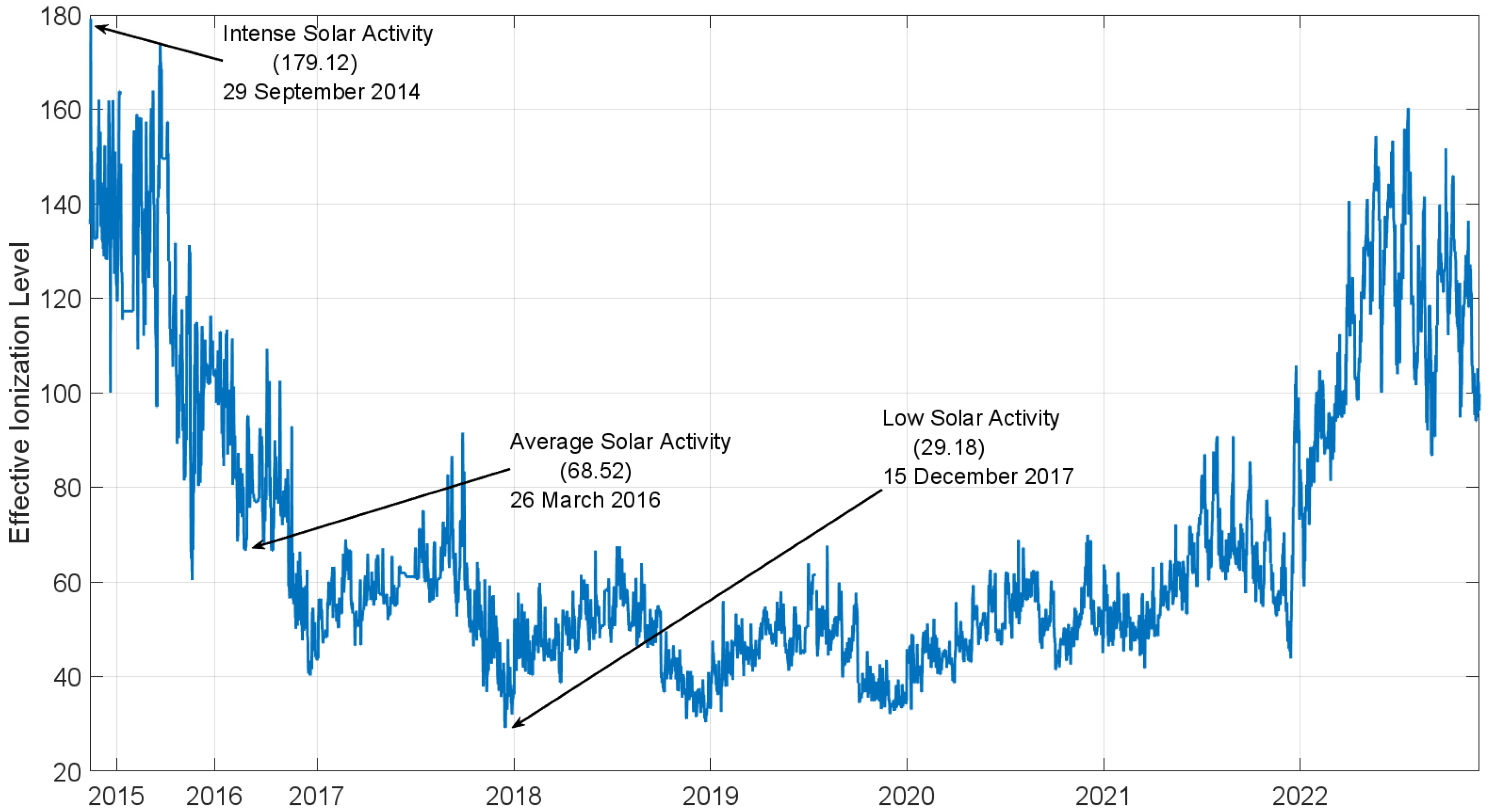
| DOY | Year | Ionization Level | Solar Activity |
|---|---|---|---|
| 272 | 2014 | 179.12 | High |
| 086 | 2016 | 68.52 | Medium |
| 349 | 2017 | 29.18 | Low |
| 012 | 2023 | 141.70 | High |
Disclaimer/Publisher’s Note: The statements, opinions and data contained in all publications are solely those of the individual author(s) and contributor(s) and not of MDPI and/or the editor(s). MDPI and/or the editor(s) disclaim responsibility for any injury to people or property resulting from any ideas, methods, instructions or products referred to in the content. |
© 2023 by the authors. Licensee MDPI, Basel, Switzerland. This article is an open access article distributed under the terms and conditions of the Creative Commons Attribution (CC BY) license (https://creativecommons.org/licenses/by/4.0/).
Share and Cite
Gioia, C.; Angrisano, A.; Gaglione, S. Neustrelitz Total Electron Content Model for Galileo Performance: A Position Domain Analysis. Sensors 2023, 23, 3766. https://doi.org/10.3390/s23073766
Gioia C, Angrisano A, Gaglione S. Neustrelitz Total Electron Content Model for Galileo Performance: A Position Domain Analysis. Sensors. 2023; 23(7):3766. https://doi.org/10.3390/s23073766
Chicago/Turabian StyleGioia, Ciro, Antonio Angrisano, and Salvatore Gaglione. 2023. "Neustrelitz Total Electron Content Model for Galileo Performance: A Position Domain Analysis" Sensors 23, no. 7: 3766. https://doi.org/10.3390/s23073766