

Invertible Privacy-Preserving Adversarial Reconstruction for Image Compressed Sensing


College of Computer Science, Chongqing University, Chongqing 400044, China
*
Author to whom correspondence should be addressed.
Sensors 2023, 23(7), 3575; https://doi.org/10.3390/s23073575
Submission received: 3 February 2023
/
Revised: 20 March 2023
/
Accepted: 27 March 2023
/
Published: 29 March 2023
(This article belongs to the Special Issue Cyber Security and AI)
Abstract
:Since the advent of compressed sensing (CS), many reconstruction algorithms have been proposed, most of which are devoted to reconstructing images with better visual quality. However, higher-quality images tend to reveal more sensitive information in machine recognition tasks. In this paper, we propose a novel invertible privacy-preserving adversarial reconstruction method for image CS. While optimizing the quality, the reconstructed images are made to be adversarial samples at the moment of generation. For semi-authorized users, they can only obtain the adversarial reconstructed images, which provide little information for machine recognition or training deep models. For authorized users, they can reverse adversarial reconstructed images to clean samples with an additional restoration network. Experimental results show that while keeping good visual quality for both types of reconstructed images, the proposed scheme can provide semi-authorized users with adversarial reconstructed images with a very low recognizable rate, and allow authorized users to further recover sanitized reconstructed images with recognition performance approximating that of the traditional CS.
1. Introduction
With the rapid development of the Internet of Things, the scale of the network becomes larger and larger, and the network environment becomes more and more complex. In the Internet of Things, the number of smart wireless sensors has increased significantly, which has brought great challenges to network communication. Problems such as energy saving, transmission efficiency, and security have gradually attracted attention. Compressed sensing (CS) [1] can help to solve the three problems of intelligent network communication simultaneously. CS is an advanced signal sampling and reconstruction method, which breaks the Nyquist sampling theorem. It can approximately restore the original signal through a few measurements, and its speed of sampling is much faster than similar traditional frameworks. It is usually used as a data encryption and compression scheme for energy-constrained wireless sensor networks.
Over the past decades, many classic traditional CS reconstruction algorithms have been proposed [2,3,4], such as the orthogonal matching pursuit algorithm (OMP) [2] and the gradient projection for sparse reconstruction algorithm (GPSR) [3]. However, such traditional reconstruction algorithms often have high computational costs, and when the sampling rate is low, it is usually difficult to obtain a reconstructed image with good quality.
Fortunately, the emergence of deep learning provides new possibilities for the reconstruction of CS. In recent years, deep learning, as a hot technology in the era of big data, has been successfully applied to the field of computer vision and has made a series of breakthroughs in tasks such as image recognition, super-resolution, and image restoration. The problem that the sparse hypothesis model in traditional CS cannot fully meet the application requirements can be solved by introducing deep learning. The CS methods based on deep learning [5,6,7] not only improve the reconstruction performance but also complete image reconstruction in a very short time, meeting the real-time requirements in real-world applications.
Most of the existing CS-related works based on deep learning are dedicated to improving the visual quality of reconstructed images, and the security they are concerned about is usually reflected in whether illegal users can restore the image content with the measurements. In fact, after the receiver has recovered high-quality reconstructed images, the privacy threat still is living. In the past, if the image content could not be recognized by human eyes, we said the image’s privacy was protected. However, in the era of big data, reconstructed images may be collected by unauthorized third parties, and then intelligent algorithms may be maliciously used for data analysis or model training, which poses a great threat to the privacy of image owners. Therefore, we propose a privacy-preserving requirement for practical applications: we hope that the reconstructed image can only meet the observation needs of the receiver’s eyes, but it cannot be used for machine tasks successfully.
From the perspective of an individual, Kashmir from the New York Times reported on Clearview.AI, a company that has collected more than 3 billion online photos and trained a large model to identify millions of citizens. However, the company finished the collection without the knowledge or explicit consent of the photo owners [8], which poses a huge threat to personal privacy. In response to this threat, Ref. [9] suggests that users add an imperceptible “cloak” perturbation before uploading their photos to social networks. As a result, the facial recognition model would make wrong judgments. From the perspective of the companies, they also want to prevent valuable internal data from being stolen by malicious employees for analyzing data or training pirated models because both of these behaviors may cause huge economic or reputational losses to the company.
Taking the above scenarios as examples, therefore, we hope that the defensive version of the reconstructed image can be viewed normally by human users. However, if receivers try to collect a large number of reconstructed images without authorization to train the pirate model, it is impossible for them to obtain a model with good performance. Of course, the receivers cannot obtain accurate and reliable privacy information by analyzing the defensive version of the reconstructed images. That is, although reconstructed images have good visual quality, they cannot be used for effective training or accuracy recognition.
This motivation reminds us of adversarial examples [10]. Nowadays, adversarial examples are a research hotspot in the security field of artificial intelligence, which aim to deceive deep neural network (DNN) models by adding imperceptible perturbations to the original samples. We use this double-edged sword in a defensive way to preserve the privacy of CS reconstructed images.
Destroying the availability of reconstructed images for machine tasks is very costly, as huge amounts of data are essential to building a well-performing deep learning model. However, both collecting data and labeling it are costly tasks, which are time-consuming and labor-consuming. Therefore, datasets are often viewed as digital property, and some companies offer them to users as paid content. If reconstructed images are simply transformed into images that cannot be trained or recognized, authorized users will lose the right to use the data properly, which causes unnecessary waste of resources. Thus, it is imperative for authorized users to restore the privacy-preserving reconstructed images to clean samples that can be used for training and recognition effectively. In other words, the adversarial reconstructed images should be reversible [11]. A reversible privacy-preserving framework for face recognition is also proposed in [12].
Inspired by [13], we pay more attention to the performance of reconstructed images in machine tasks. However, our goal is not to improve the recognition performance of reconstructed images but to achieve privacy protection by reducing their recognition accuracy. Therefore, we propose a novel invertible privacy-preserving adversarial reconstruction method for image CS based on adversarial examples (IPPARNet). We divide the users into two categories: semi-authorized users and authorized users. The adversarial reconstruction network takes the measurements as input and then outputs the reconstructed image, which is an adversarial sample. Such reconstructed images could be obtained by a semi-authorized user. Although they can be recognized normally by human eyes, the DNN models will be misled by them and make incorrect inferences, so as to achieve the purpose of privacy protection. At the same time, we also consider the invertibility of machine task availability. For authorized users, they can employ an additional restoration network to restore the adversarial sample to a sanitized sample which is helpful for machine tasks, avoiding the secondary transmission of available data. The authors of [13] point out that machine users pay more attention to machine metrics such as image recognition accuracy, rather than visual quality. Inspired by this, we also regard recognition accuracy as an extra optimization goal of the authenticated restoration network to improve the recognizability of recovered clean samples.
The main contributions of this paper are summarized below:
- We consider both the visual quality of reconstructed images and their ability to confuse DNN models during the reconstruction process of CS so that the reconstructed images have the ability to fool the DNN models at the time of generation.
- We propose a privacy-preserving reconstruction method for image CS based on adversarial examples for users with two levels. While guaranteeing the visual quality of the reconstructed images, we take the machine recognition metric as the starting point and focus on the privacy needs of different users. We not only follow the original adversarial samples but also consider the invertibility of task availability of reconstructed images. Specifically, semi-authorized users can only obtain adversarial reconstructed images, which protects user privacy by reducing the accuracy rate of the recognition models. In contrast, authorized users can restore sanitized reconstructed images from the adversarial reconstructed images for more efficient model training or more accurate data analysis, enabling invertibility for machine task availability.
- The good performance of the IPPARNet is demonstrated with extensive experiments. Keeping good visual quality, the recognizability of adversarial reconstructed images is low enough to avoid being used illegally by malicious users, while the sanitized reconstructed images can reach an approximate or even slightly higher recognition rate compared with that of the original CS reconstructed images.
The rest of this paper is organized as follows. In Section 2, we review the related work of CS and adversarial examples. In Section 3, we introduce the proposed scheme in detail. Section 4 provides the experimental setting and presents the experimental results. Finally, our work is concluded in Section 5.
2. Related Works
2.1. Compressed Sensing
2.1.1. Traditional Compressed Sensing
The proposal of CS breaks the Nyquist–Shannon theorem and provides a concise and efficient signal acquisition paradigm. The theory of CS points out that as long as the original signal x is sparse in a certain transform domain, it is possible to project the transformed high-dimensional signal onto a low-dimensional space with a measurement matrix that is uncorrelated with the orthogonal transform basis . Then, by solving an optimization problem, the original signal can be reconstructed with high probability from the measurements .
The formulation of the CS measurement process can be expressed as:
where s is the sparse coefficient of the original signal x with respect to the basis Ψ. In addition, m << n and is called the sampling rate. The commonly used measurement matrices include structured random matrix, random Gaussian matrix, random Bernoulli matrix, etc. From Equation (1), it can be seen that the computational complexity of the measurement process of CS is fairly low, which is one of its significant advantages.
The reconstruction of CS can be viewed as the inverse process of measuring, and the original image can be reconstructed by seeking the sparsest solution of Equation (1). Although it is an under-determined problem, it can be converted into a problem of minimizing norm due to satisfying the sparsity of the signal, i.e., solving
However, solving Equation (2) is an NP-Hard problem, so it is usually solved iteratively using an approximation algorithm. The commonly used traditional reconstruction algorithms can be divided into two main categories, one is based on convex optimization class algorithms, such as basis pursuit algorithm (BP), GPSR [3], and ISTA-Net [7]. The second is based on greedy algorithms, such as the matching pursuit (MP) algorithm and OMP [2].
Although traditional CS greatly reduces the computational complexity in the measurement process, its reconstruction cost is very expensive. In practical applications, the computationally complex reconstruction work is usually outsourced to cloud servers with abundant computing resources. However, the heavy computation of traditional reconstruction algorithms has not been improved from the root cause.
2.1.2. Compressed Sensing Based on Deep Learning
With the rapid development of deep learning, DNNs are applied to implement CS, which not only further improves the reconstruction quality, but also significantly increases the reconstruction speed. In 2015, Mousavi et al. [14] introduced deep learning into CS with fully connected networks for the first time and proposed a stacked denoising autoencoder (SDA) to capture the statistical correlation between different elements of the signal, thereby improving the quality of the reconstructed signal. Compared with the fully connected network, the convolutional neural network (CNN) reduces the number of parameters and enhances the model expression ability with mechanisms such as parameter sharing and local connectivity. In [15], Kuldeep Kulkarni et al. combined CS with CNN for the first time, and proposed a non-iterative block CS (BCS) [16] reconstruction network named ReconNet. In [17], after the reconstructed linear map from the measurement, a residual network was introduced to narrow the gap between the initial reconstructed image and the original image, leading to a higher reconstruction quality.
However, the above schemes only consider the reconstruction process and do not involve the measurement process, and they use the same measurement matrices as the traditional CS algorithms. In [18], based on ReconNet, a fully connected layer is used to simulate the measurement process, and an efficient measurement matrix could be adaptively learned. In this way, the measurements retain more image structure information, and complex manual design is avoided at the same time. By jointly training the new network consisting of a fully connected layer and ReconNet, visually better-quality images can be reconstructed. Based on BCS, [19] employs deep CNN to achieve sampling and reconstruction, and also trains the sampling network and the reconstruction network in an end-to-end way to quickly restore the reconstructed image with better quality. The authors of [20] further optimize the learned measurement matrices, and propose a {0, 1}-binary matrix and a {−1, +1}-bipolar matrix, which are more convenient for storage and hardware implementation in practical applications. In addition, residual learning is also introduced for better reconstruction.
As mentioned above, most deep learning-based CS schemes focus on two issues: the first is how to learn an effective measurement matrix; the second is how to reconstruct images with better quality and higher speed. However, Ref. [13] points out that in some scenarios, reconstructed images are not used for human viewing but for tasks conducted by machine users. Therefore, we should pay attention to what metrics the machine users are concerned about, such as recognition accuracy. Different from [13], it takes recognition accuracy as an extra optimization goal for CS reconstruction networks, aiming to further improve the recognition rate while reconstructing. In this paper, although we also focus on recognition accuracy, we hope that the reconstructed image is an adversarial sample as it is generated, which has the innate ability to fool DNN models. Thus, the adversarial reconstructed images can avoid being abused by unauthorized users for data analysis or model training, and play an important role in privacy protection.
2.2. Adversarial Examples
In 2013, Szegedy et al. [21] first proposed the concept of adversarial samples. That is, after applying an imperceptible perturbation to the original image, the DNN models will wrongly classify the image with high confidence. Such perturbation is called adversarial perturbation, and the image to which the adversarial perturbation is added is called an adversarial sample.
In terms of the model prediction errors, the adversarial sample attack can be divided into two categories: untargeted adversarial samples and targeted adversarial samples. The former means that the adversarial sample can be misclassified by the model as any class other than its real class, while the latter refers to the adversarial sample that can be misclassified as the wrong class specified by the attacker. In this paper, we focus on untargeted adversarial samples.
In terms of the generation manner, adversarial samples can be divided into the following three categories: gradient-based, optimization-based, and generation-based.
In [22], Goodfellow et al. proposed a fast method for generating adversarial samples based on gradients called the fast gradient sign method (FGSM). The method adds a small perturbation whose elements are equal to the sign of the elements of the gradient of the loss function with respect to the input, and rapidly increases the loss in a single step, so as to deceive the DNN models. Subsequently, the gradient direction-based adversarial sample generation methods have been widely studied, such as the basic iterative method (BIM) [23] and the projected gradient descent (PGD) [24]. The BIM provides more robust adversarial examples by modifying the one-step update of FGSM to a multi-step iteration. While the PGD, using gradient projection, is considered the strongest first-order adversarial attack method available.
In [10], Carlini et al. considered generating adversarial samples as an optimization problem and proposed the Carlini and Wagner attack (C&W) which continuously optimizes the perturbations according to the set optimization decline, thus achieving a more efficient adversarial sample with smaller perturbations.
However, the above algorithms based on iterative optimization generally suffer from high computational cost and slow running speed. In recent years, with the development of generative adversarial networks (GAN) [25], the generation of adversarial samples has become more diverse. Based on GAN, Xiao et al. [26] proposed a fast adversarial perturbation generation method called AdvGAN. The generator G takes the original image x as the input and outputs the adversarial perturbation G(x). Then, the perturbation is superimposed on the original image to obtain the adversarial sample x + G(x). The mutual game between the discriminator and the generator drives the visual similarity of the adversarial samples and the original images. Since this scheme does not require iterative optimization and generates the adversarial sample in a single forward pass at the inference stage, it significantly improves the generation speed of the adversarial sample while guaranteeing the success rate of the attack and the image quality. AdvGAN++ [27], based on AdvGAN, proposes to make full use of the potential features of the original image to generate adversarial samples. In this paper, the adversarial reconstructed image is an adversarial sample generated by the generation-based method.
3. Proposed Method
3.1. Overview
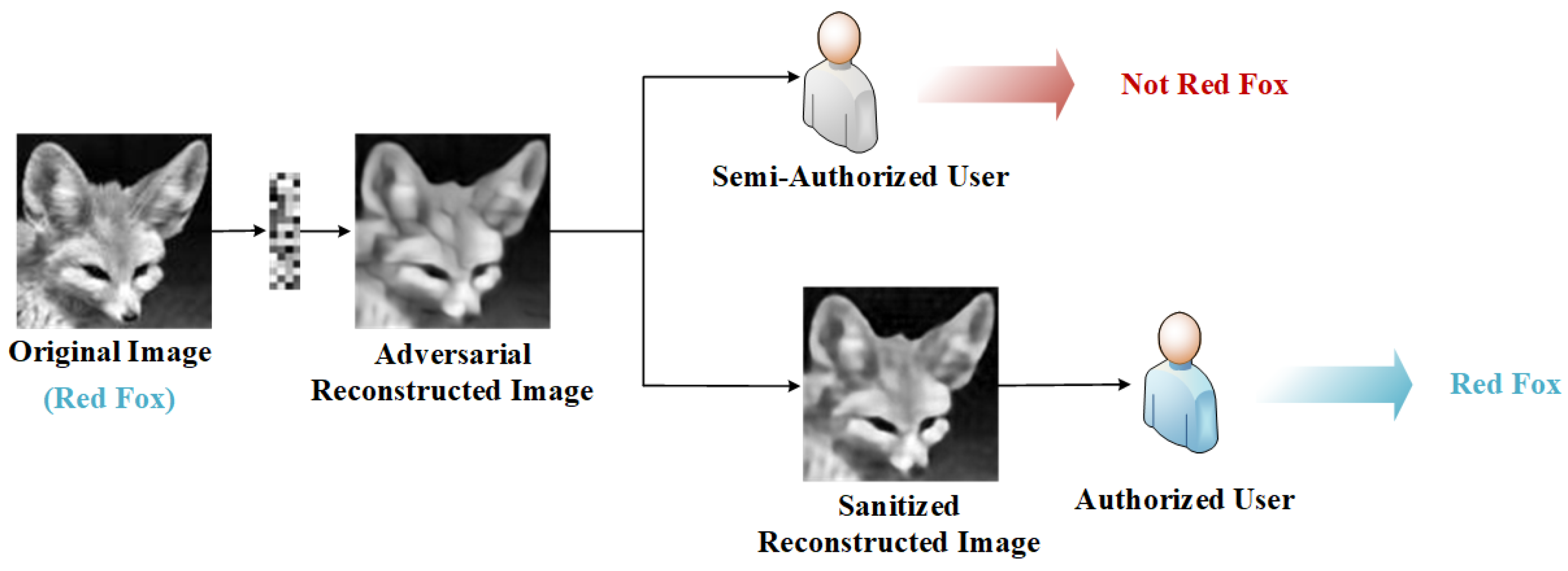
Suppose is the original dataset with N images, where represents the original image with the serial number of i, and represents the classification label corresponding to . The is sampled to obtain a measurement vector , then receivers can reconstruct the approximate image of the original image with . Similarly, the reconstructed image dataset can be expressed as . In most cases, we hope the reconstructed image to be visually similar to as much as possible, pursuing higher visual quality. However, images with high visual quality often bring privacy leakage problems. For example, when =, these reconstructed images can be analyzed by unauthorized models, or a large number of them can be collected by illegal users for model training.
Therefore, we propose a novel privacy-preserving adversarial reconstruction framework for CS, as shown in Figure 1. We designed it for semi-authorized users and authorized users. Specifically, the adversarial reconstructed images , which are reconstructed from the measurement vector and could protect the privacy of the original image , can be obtained by all users.
Our goal is to make visually similar to as much as possible; however, for the recognition models based on deep neural networks, the corresponding label of is different from . That is, the image is an adversarial example at the beginning of the reconstruction. In this way, although semi-authorized users obtain visually useful images, they cannot use such images to perform data analysis tasks well, nor can they train effective models. That is to say, while ensuring the practicability of the reconstructed images, we also protect their privacy. When authorized users have task needs, they can restore the adversarial reconstructed image to the sanitized image with the restoration network R. Similarly, for human eyes, the visual difference between and the reconstructed image of CSNet should be indistinguishable. However, the classification labels of and should be the same, that is,. In this way, the sanitized image can not only be recognized by human beings, but also be beneficial to machine users for downstream tasks. In this paper, we take the task of recognizing categories as an example. It is worth noting that, inspired by [13], we also pay more attention to the machine users, that is, is more helpful to improve recognition performance than the reconstructed image of traditional CS.
3.2. Network Architecture
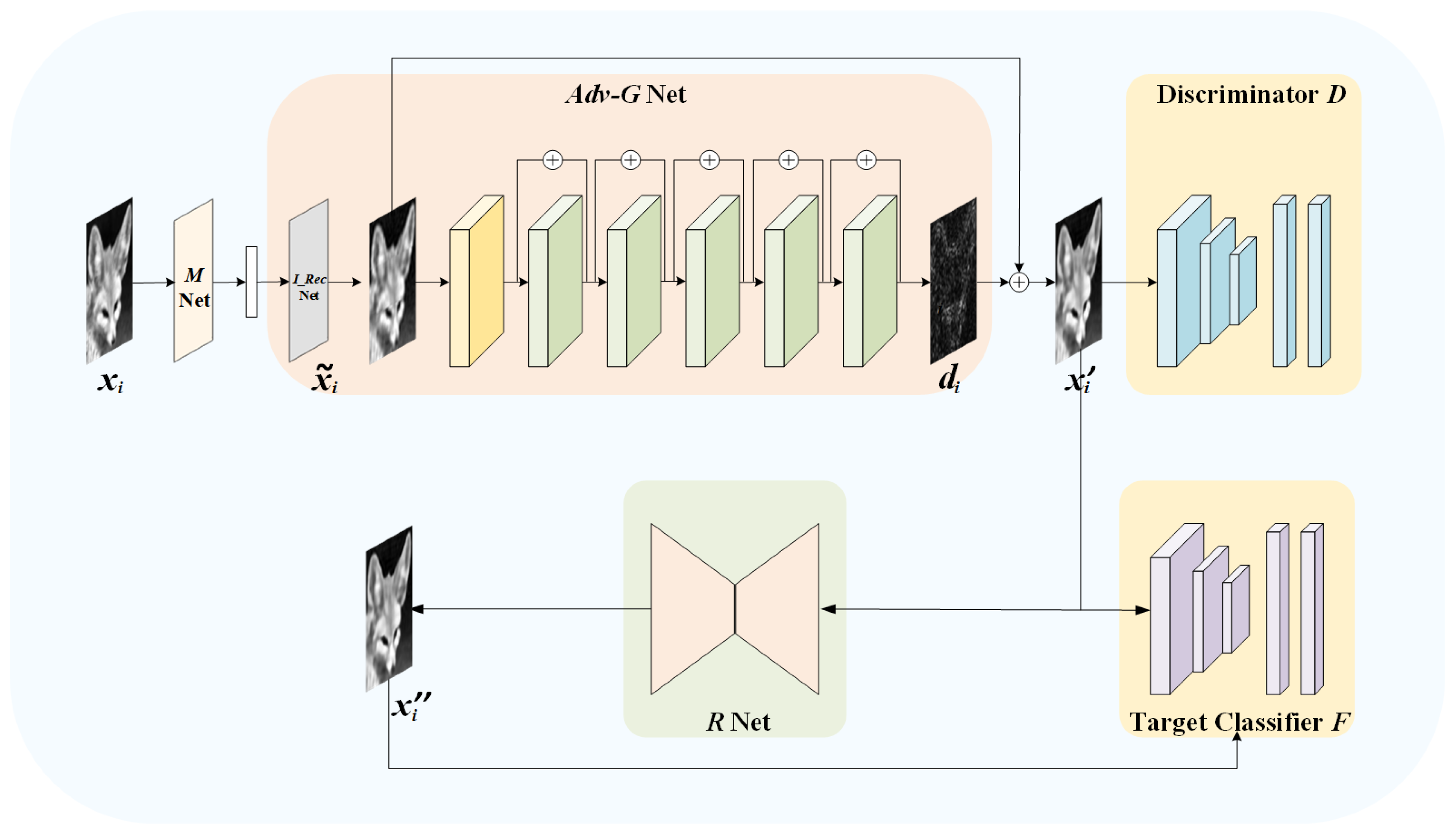
Our model framework consists of a measurement network , an adversarial reconstruction network -, a discriminator network , a restoration network , and several pre-trained target classifiers, where the subscripts , , , and are the trained parameters. For simplicity, if there is no ambiguity, we omit the subscripts. Figure 2 shows the overall architecture of our proposed model.
Formally, the measurement process can be expressed as:
After the original image is measured by the measurement network , the measurement vector is the output.
As for reconstruction, our proposed IPPARNet includes two stages. The first reconstruction stage can be defined as:
With the input , the − network outputs the adversarial reconstructed image . Both networks and − are derived from CSNet [20].
We employ several pre-trained classifiers as a joint target network F. should have the ability to induce the ensemble target network F to make wrong inferences while ensuring good image quality. At the same time, we introduce a discriminator D to encourage the adversarial reconstructed image to achieve a high visual quality.
The second reconstruction stage can be described as:
With the additional restoration network , authorized users can take the adversarial reconstructed image as the input, and further restore the sanitized image . For the target network , can achieve a high recognition accuracy, which is more conducive to subsequent recognition tasks.
3.2.1. Measurement Network:
Based on BCS, we firstly divide the original image into non-overlapping blocks of size B × B × c, where c represents the number of channels. As shown in Equation (1), the measurement process of traditional CS can be expressed as . Regarding each row of the measurement matrix as a filter, the measurement process can be done by a convolutional layer without biases.
For the non-overlapping measurement process, the convolutional layer measures the original image with filters of size B × B × c and a stride of B. When the sampling rate is , the convolutional layer contains n = filters. An image block of size B × B × c is fed into the measurement network to obtain the output measurement vector of size 1 × 1 × n. Furthermore, there is no bias in each filter. The measurement network can learn an efficient measurement matrix adaptively, thereby avoiding complicated and possibly inefficient manual design of the measurement matrix.
3.2.2. Adversarial Reconstruction Network: -
This network can be divided into two components: the initial reconstruction network (referred as ) and the deep reconstruction network (referred as ).
In the traditional BCS, the pseudo-inverse matrix is usually used to reconstruct the primary reconstructed image from the measurement value. The implementation of the corresponding network is similar to that of the measurement network. We can also obtain a rough reconstruction of the image with the network , which includes a convolutional layer with filters ignoring the bias.
In the network, c filters of size 1 × 1 × n and a stride of 1 can be used to obtain reconstructed image blocks. However, the output of each image block is still a vector at this time, so we need a combination layer to reshape it to a block of size B × B × c and then concatenate these blocks together to obtain the reconstructed image. Since the network does not employ any activation layer, the initial reconstruction is a linear operation. The linear mapping produces a relatively good initial reconstructed image with fast speed and low computational cost, but its visual quality is poor and has obvious block artifacts.
Therefore, we hope to further narrow the gap between and with the network . The network learns the residual , and the final output of the adversarial reconstruction network - is . For the so-called “adversarial reconstruction”, we hope that the learned perturbation , on the one hand, can further improve the visual quality of the output image of network . On the other hand, when it is added to , can induce the target network to make wrong predictions, that is to say, has the ability to mislead the target model at the moment of generation. For the architecture of , we replace residual blocks with those in [28].
3.2.3. Restoration Network: R
U-Net [29] is widely used in image processing tasks with DNNs. It uses skip connections to combine the high-level semantic feature maps from the decoder with the corresponding low-level detailed feature maps from the encoder, which is helpful to generate high-quality images. Since the goal of the restoration network is to obtain the sanitized image with the best possible recognition performance while receiving the adversarial reconstructed image , the network employs U-net as the backbone. Specifically, its encoder includes four encoding segments, and each segment consists of two convolutions, each of which is followed by a rectified linear unit (ReLU) and a 2 × 2 max pooling operation with stride 2 for down sampling. In addition, each encoding segment doubles the number of feature channels. Correspondingly, the decoder also consists of four decoding segments. Each decoding segment contains a deconvolution layer with stride 2, a connection with the corresponding feature maps from the encoding segment, and 2 convolution layers, each followed by a ReLU. Moreover, each decoding segment reduces the number of channels by half. Finally, the output image of the decoder has the same size as the original image.
3.2.4. Discriminator:
Our discriminator is designed as a common 4-layer CNN which outputs a value from 0 to 1 by the sigmoid function. It is used to distinguish between the original image and the adversarial reconstructed image generated by the network -. After the continuous game between the network - and , could have the better visual quality.
3.2.5. Ensemble Target Networks:
3.3. Loss Functions
As mentioned before, we represent the original dataset as , where represents the original images with the serial number of i, and represents the classification label corresponding to .
: The loss function of network - mainly includes four components: the reconstruction loss , the adversarial loss , the perception loss , and the classification loss .
In order to make the output image of the network - similar to the original image on the pixel level, following most deep learning-based image restoration methods, we use the norm between and to constrain the difference of them. For the reconstruction loss, we have
To further narrow the difference between and , we employ the idea of generative adversarial network and introduce the discriminator . With the help of the discriminator D, the network - is trained in an adversarial way. The adversarial loss can be described as:
Furthermore, we introduce the perceptual loss [32], which is based on feature extractors of VGG16, to optimize the similarity of and in the feature space. The perception loss can be express as:
Specifically, we calculate the Euclidean distance between feature maps of and from the second max-pooling layer. That is, j of in Equation (8) is 2.
We take the visual quality and recognition metrics into account at the same time. However, unlike the goal of [13], while they try to improve the recognition performance of the reconstructed images, we attempt to make the adversarial reconstructed images mislead the target network. Therefore, we use the negative cross-entropy to encourage to be classified wrongly by the ensemble target networks . We take the average loss of the three target classifiers as the final classification loss ,
where is the cross-entropy loss function, , which is used to calculate the cross entropy between the predicted label and the ground truth .
In summary, the total loss of the adversarial reconstruction network - is defined as follows:
where , , and are hyper-parameters that play a very significant role in the training process.
: The same as in [25], the discriminator is used to distinguish whether the image is the original one or the reconstructed one, and its loss is:
: The goal of the restoration network is to output the restoration image that is not only visually similar to the original image , but also beneficial for machine recognition tasks. We still use the norm to optimize ,
To facilitate the correct recognition of the sanitized image by the ensemble target networks, we introduce the positive cross-entropy loss ,
Similarly, we take the average loss of the three target classifiers as the final classification loss. The loss function of the restoration network R can be expressed as:
where is a hyper-parameter.
In summary, the total loss of the proposed IPPARNet is defined as follows:
where is a hyper-parameter.
3.4. Training and Inference
In the training process of the proposed IPPARNet, we alternately train the discriminator , the adversarial reconstruction network -, and the restoration network . Specifically, we optimize the discriminator by minimizing Equation (11) and then optimize the total loss . In this way, both the adversarial reconstruction network - and the restoration network can generate images with good visual quality, but the former hinders the prediction of the recognizer while the latter can increase the recognition accuracy.
In the inference process, there is no need to use the discriminator . Feeding the measurement vector into the adversarial reconstruction network -, the adversarial reconstructed image is obtained, which can be comprehended by semi-authorized users with human eyes. However, for machine users, cannot be recognized accurately, nor can it be used for meaningful training. Therefore, even if malicious users collocate a mass of adversarial reconstructed images, they cannot analyze them effectively or use them to train a model with good performance. However, when the authorized user has task needs, can be fed into the recovery network to output the sanitized image that can improve the performance of the machine users in the recognition tasks.
It can be seen that the proposed method mainly introduces a discriminator and a restoration network to the original CSNet, achieving our goal by designing loss functions carefully. That is to say, there is no need to change the related hardware for the measuring and reconstructing of the original CS.
4. Experiment and Results
4.1. Experimental Setting
In the experiments, we use a personal computer configured with an Intel i7-10700 CPU, a NVIDIA RTX 2080 graphics card, and 32 GB of memory. PyTorch1.11.0 is used to implement all methods.
Following [13], we select 30 classes of images from the original ImageNet database and scale them to the size of 96 × 96 to obtain the Tiny-ImageNet as the dataset for our experiment. Specifically, the training set contains 38,766 images and the test set includes 1500 images, while each class has 50 images. Since [20] used a grayscale dataset, all images in this experiment received grayscale processing to facilitate performance comparison.
For a fair performance evaluation, firstly, we train the CSNet [20] network in this environment with images divided into 32 × 32 blocks. Then, three classic classification networks, VGG16, ResNet50, and DenseNet121, are trained with the Tiny-ImageNet dataset.
Finally, we train the proposed IPPARNet model with the pre-trained CSNet network and the three classification networks. While training, we fix the parameters of the classifiers and alternately train the discriminator network and the adversarial network -. Playing the two-player minimax game, the discriminator can prompt the adversarial reconstruction network - to generate adversarial reconstructed images that are more similar to the original images. At the same time, the adversarial reconstruction network - and the restoration network are jointly trained to obtain better restoration of the sanitized images.
The optimization algorithm Adam is employed and the batch size is 32. The learning rate of adversarial network -, recovery network , and discriminator is set to 0.0001, which is reduced to 0.1 times every 50 rounds. When the sampling rate is 0.1, the hyperparameters are set as follows: = 0.001, = 0.001, = 0.0005, = 0.001, and = 2.
4.2. Results and Analysis
4.2.1. Benchmark
We not only take account of the quality of the CS reconstructed images and the ability to fool the DNN models, but also have thought to reverse the adversarial reconstructed images to sanitized samples. However, to the best of our knowledge, there is no previous study dealing with the above tasks. Therefore, we use the reconstructed images from the CSNet as the benchmark, then evaluate the performance of the adversarial reconstructed images and the restored sanitized images . Specifically, , , , and that appear in the following paper represent the set of all , , , and on the test set, respectively.
For evaluation, we use 1500 grayscale images of size 96 × 96 from the Tiny-ImageNet test set and employ peak signal-to-noise ratios (PSNRs) and recognition accuracy as evaluation metrics.
At first, we test the performance of the pre-trained VGG16, ResNet50, and DenseNet121 classifiers for 1500 Tiny-ImageNet test images. Table 1 shows the recognition accuracy of the original test set on the three classification networks. The row of “Average” means the average recognition rate of the three classifiers. Compared with the trained one on all ImageNet database, the recognition rate of the three recognition networks we trained is much lower. This is because our training set is much less than the ImageNet database, accounting for less than 1/30. Therefore, getting relatively low recognition rate is a reasonable phenomenon.
Then, setting the sampling rate as 0.1, 0.2, 0.3 and 0.5, we employ the CSNet to implement reconstruction for the test set of the Tiny-ImageNet. Table 2 shows the image quality of the CSNet reconstructed images under different sampling rates with the metric PSNR. Table 3 shows the recognition rates of VGG16, ResNet50, and DenseNet121 for
One can see from Table 2 and Table 3 that with the increase in sampling rate, the PSNR values and recognition accuracy of CSNet reconstructed images were improved. Compared with the original image, at different sampling rates, the recognition accuracy of the reconstructed image on the three classifiers decreased to varying degrees. However, even when the sampling rate is 0.1, the reconstructed images can achieve a recognition accuracy of 41–61% on the three classifiers. While the sampling rate is 0.5, their recognition accuracy is almost equal to that achieved on the original images. This means that malicious users can acquire a lot of sensitive information from CSNet reconstructed images, , which poses a great privacy threat.
4.2.2. Performance Evaluation
The goal of the proposed IPPARNet is to take the machine recognition metric into account while retaining good visual quality. On the one hand, the adversarial reconstructed images can mislead the target classifiers, making it difficult for semi-authorized users to abuse them effectively, so as to achieve the goal of privacy protection. On the other hand, authorized users can restore sanitized images from , and the recognition accuracy can be improved as high as possible, which is helpful for the machine’s subsequent recognition tasks. That is to say, while keeping a reasonable PSNR, for the adversarial reconstructed images , the lower the recognition rate, the better the performance. However, for the sanitized images , the higher the recognition rate, the better the performance.
- Analysis of Recognition Accuracy
At different sampling rates, the recognition rates of VGG16, ResNet50, and DenseNet121 classifiers for adversarial reconstructed images and sanitized images are shown in Table 4. It can be observed that for each sampling rate, the recognition rates of the adversarial reconstructed images are significantly lower than that of the CSNet reconstructed images . Take the sampling rate of 0.1 as an example. The recognition rates of , which is generated by our adversarial reconstruction network, on the three classifiers VGG16, ResNet50, and DenseNet121 are not more than 1/10, which are 6.0%, 10.0%, and 7.6%, respectively. Compared with , the recognition rates of are relatively reduced by 85.3%, 83.6%, and 86.2%. When setting the sampling rate as 0.2, 0.3, and 0.5, the average recognition rate of adversarial reconstructed images on the three classifiers drops from 71.5%, 74.0%, and 78.6% to 8.8%, 12.8%, and 13.5%, respectively. It can be seen that the relative declines are all greater than 82.0%, which results in semi-authorized machine users being unable to recognize these adversarial reconstructed images precisely. In other words, semi-authorized machine users are prevented from performing effective data analysis and model training tasks, and the privacy of images is protected.
However, authorized users can obtain sanitized reconstructed images with the additional restoration network. When the sampling rate is 0.1, the corresponding recognition rates on the three classifiers are 49.2%, 62.0%, and 55.6%, respectively, which are slightly higher than the recognition rates of reconstructed by the CSNet. At other sampling rates, the average recognition rates of the sanitized reconstructed images on the three classifiers can reach 69.6%, 70.3%, and 74.7%, which are approximate to that achieved by . Obviously, contributes to the machine recognition tasks.
- 2.
- Analysis of Image Visual Quality
Table 5 shows the PSNR values of the CSNet reconstructed images , the adversarial reconstructed images , and the sanitized images . Take the sampling rate of 0.1 as an example. Compared with , the PSNR value of our adversarial reconstructed images is only reduced by 0.39 dB. At different sampling rates, the PSNR values drops by 0.2–6.1%. When the sampling rate is 0.5, the PSNR value remains at 27.82 dB, which still provides a good visual effect for human eyes. In comparison, the PSNR values of the sanitized images have a smaller decrease. In the case of sampling rate 0.1, it is only 0.06 dB lower than . Since the PSNR value of is greater than that of at the same sampling rate, we infer that has better visual quality than .
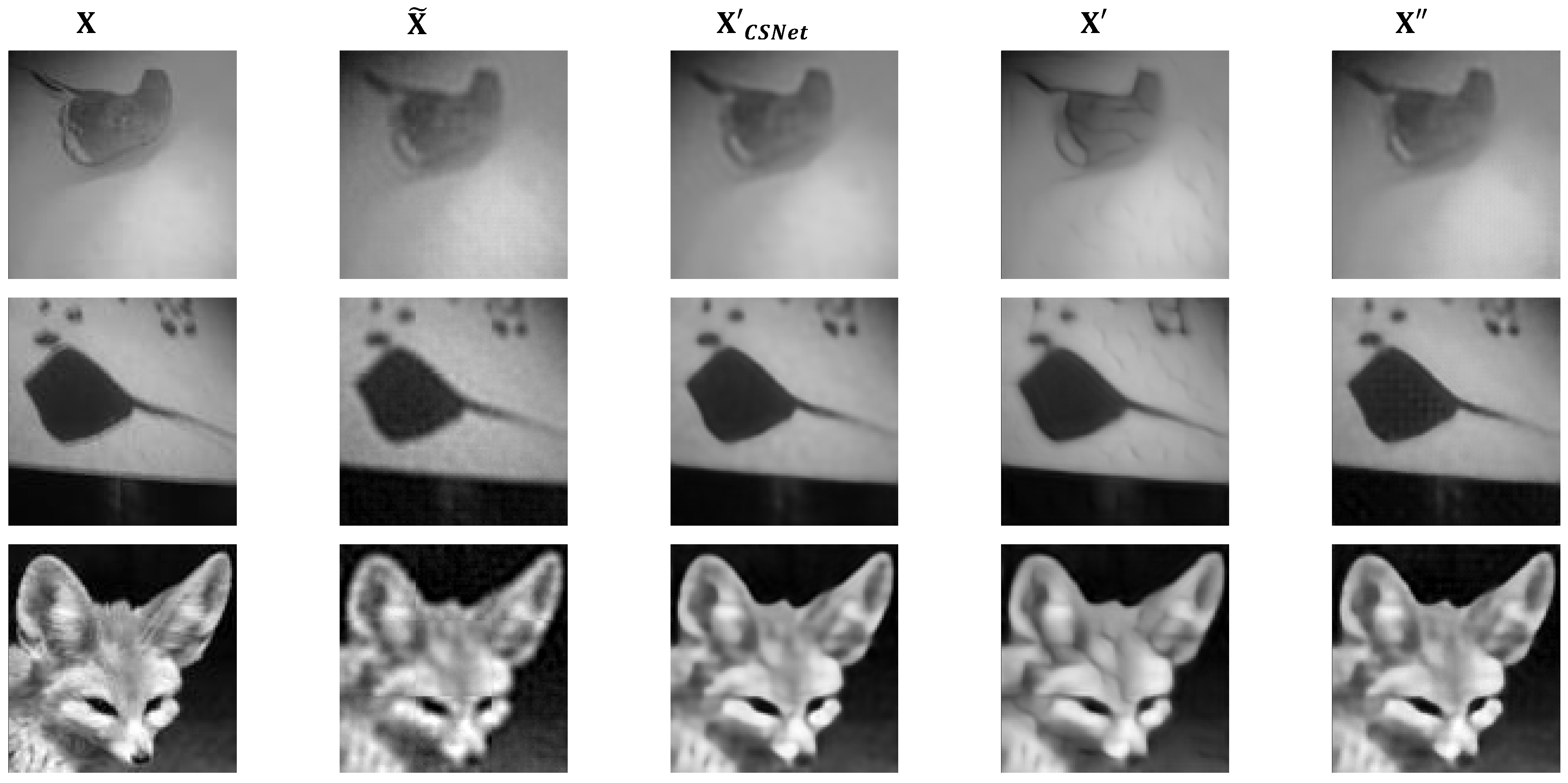
To perceive the visual quality of the image intuitively, three images from the Tiny-ImageNet test set were randomly selected as representatives. Figure 3 illustrates the original images , the corresponding initial reconstructed images , the reconstructed images of CSNet, our adversarial reconstructed images , and the restored sanitized images of the three images.
It can be observed that our adversarial reconstructed images are not disturbed significantly compared with CSNet reconstructed images and the sanitized images restored by authorized users are visually indistinguishable from . Both and have good visual quality for human beings and is better.
During the reconstruction, the network of the CSNet learns a linear mapping to obtain relatively good initial reconstructed images, . Then, with a nonlinear network , the residual between the initial reconstructed images and the original images is learnt, which can eliminate the block artifacts of and further improve the visual quality simultaneously. However, the adversarial reconstruction network - aims to learn a perturbation that makes the final reconstructed images have the ability to deceive DNN models with this nonlinear network. That is, by adding the perturbation, the final reconstructed images can induce the recognizer to make wrong judgments while ensuring it has good visual quality.
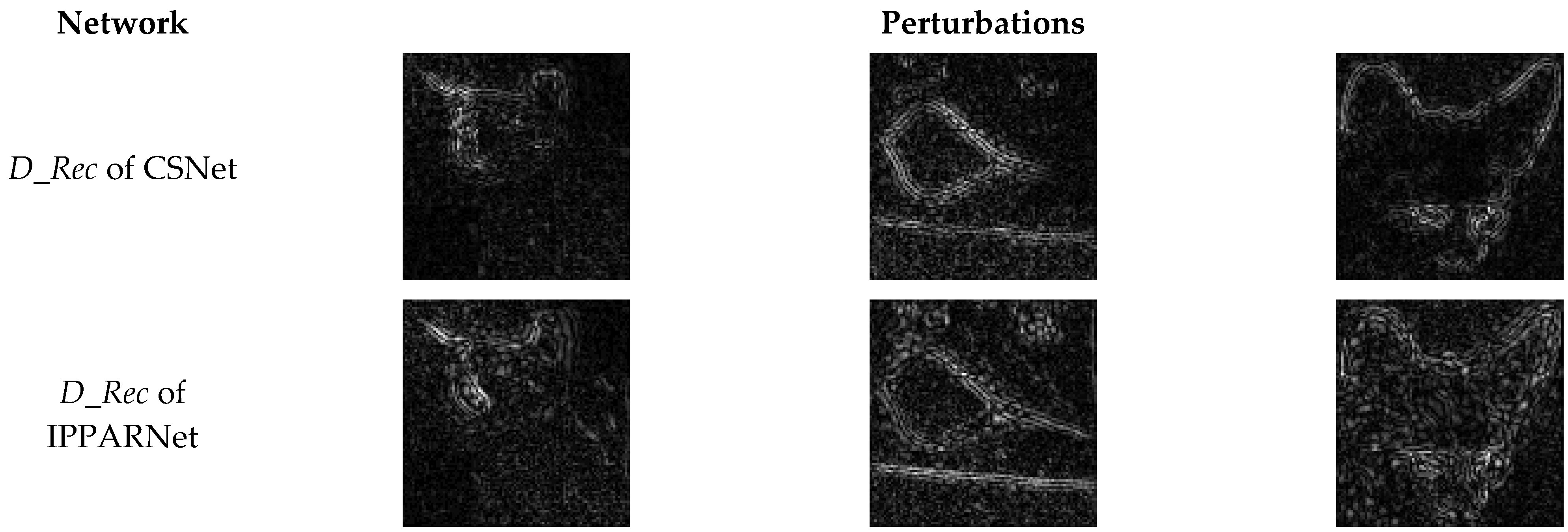
Figure 4 shows the perturbations learned by the network of CSNet and the proposed IPPARNet. It can be seen that in our method, the learned perturbations cannot only eliminate block artifacts and supplement the contour details, but also acquire additional adversarial perturbations.
In summary, with the proposed IPPARNet, under the premise of ensuring good visual quality, the recognition rate of the adversarial reconstructed images can be reduced by more than 82% compared with CSNet reconstructed images , while authorized users can restore sanitized images which achieve the approximate recognition accuracy of the .
5. Conclusions
In this paper, we propose a novel image CS reconstruction method that supports inversible privacy protection. On the one hand, we use adversarial samples as a weapon of privacy protection. In the process of image CS reconstruction, we simultaneously consider the visual quality of the reconstructed image and its ability to deceive the DNN models. On the other hand, we jointly train both the adversarial reconstruction network and the restoration network to ensure the invertibility of adversarial reconstructed images. Numerous experimental results show that our method can generate adversarial reconstructed images with a high attack success rate and sanitized reconstructed images with better recognition accuracy, while maintaining good visual quality. The adversarial reconstructed images can protect private data from malicious users, while the sanitized reconstructed images can safeguard the legitimate rights of authorized users and avoid unnecessary resource wastage. In future work, we will explore how to further improve the recognition accuracy of the sanitized reconstructed images.
Author Contributions
Conceptualization, D.X. and Y.L.; methodology, Y.L. and M.L.; software, Y.L.; validation, D.X., Y.L., and M.L.; formal analysis, Y.L. and M.L.; investigation, Y.L.; resources, Y.L.; data curation, Y.L.; writing—original draft preparation, Y.L.; writing—review and editing, D.X. and Y.L.; visualization, Y.L.; supervision, D.X.; project administration, D.X.; funding acquisition, D.X. All authors have read and agreed to the published version of the manuscript.
Funding
This research was funded by the National Natural Science Foundation of China (Grant No. 62072063) and the project supported by Graduate Student Research and Innovation Foundation of Chongqing, China (Grant No. CYB22063).
Institutional Review Board Statement
Not applicable.
Informed Consent Statement
Not applicable.
Data Availability Statement
All experiments from this paper are performed on public datasets.
Conflicts of Interest
The authors declare no conflict of interest.
Abbreviations
The following abbreviations are used in this manuscript:
| CS | Compressed sensing |
| OMP | Orthogonal matching pursuit |
| GPSR | Gradient projection for sparse reconstruction |
| DNN | Deep neural network |
| BP | Basis pursuit |
| MP | Matching pursuit |
| SDA | Stacked denoising autoencoder |
| CNN | Convolutional neural network |
| BCS | Block compressed sensing |
| FGSM | Fast gradient sign method |
| BIM | Basic iterative method |
| PGD | Projected gradient descent |
| GAN | Generative adversarial networks |
| ReLU | Rectified linear unit |
References
- Donoho, D.L. Compressed sensing. IEEE Trans. Inform. Theory 2006, 52, 1289–1306. [Google Scholar] [CrossRef]
- Tropp, J.A.; Gilbert, A.C. Signal Recovery from Random Measurements Via Orthogonal Matching Pursuit. IEEE Trans. Inform. Theory 2007, 53, 4655–4666. [Google Scholar] [CrossRef] [Green Version]
- Figueiredo, M.A.T.; Nowak, R.D.; Wright, S.J. Gradient Projection for Sparse Reconstruction: Application to Compressed Sensing and Other Inverse Problems. IEEE J. Sel. Top. Sign. Process. 2007, 1, 586–597. [Google Scholar] [CrossRef] [Green Version]
- Ji, S.; Xue, Y.; Carin, L. Bayesian compressive sensing. IEEE Trans. Signal Process. 2008, 56, 2346–2356. [Google Scholar] [CrossRef]
- Zhou, S.; He, Y.; Liu, Y.; Li, C.; Zhang, J. Multi-Channel Deep Networks for Block-Based Image Compressive Sensing. IEEE Trans. Multimed. 2021, 23, 2627–2640. [Google Scholar] [CrossRef]
- Lohit, S.; Kulkarni, K.; Kerviche, R.; Turaga, P.; Ashok, A. Convolutional Neural Networks for Noniterative Reconstruction of Compressively Sensed Images. IEEE Trans. Comput. Imaging 2018, 4, 326–340. [Google Scholar] [CrossRef] [Green Version]
- Zhang, J.; Ghanem, B. ISTA-Net: Interpretable Optimization-Inspired Deep Network for Image Compressive Sensing. In Proceedings of the IEEE Conference on Computer Vision and Pattern Recognition, Salt Lake City, UT, USA, 18–21 June 2018; pp. 1828–1837. [Google Scholar]
- Hill, K. The secretive company that might end privacy as we know it. The New York Times, 18 January 2020. [Google Scholar]
- Shan, S.; Wenger, E.; Zhang, J.; Li, H.; Zheng, H.; Zhao, B.Y. Fawkes: Protecting Privacy against Unauthorized Deep Learning Models. In Proceedings of the 29th USENIX Conference on Security Symposium, Boston, MA, USA, 12–14 August 2020; pp. 1589–1604. [Google Scholar]
- Carlini, N.; Wagner, D. Towards Evaluating the Robustness of Neural Networks. In Proceedings of the IEEE Symposium on Security and Privacy, San Jose, CA, USA, 22–26 May 2017; pp. 39–57. [Google Scholar]
- Chen, K.; Zeng, X.; Ying, Q.; Li, S.; Qian, Z.; Zhang, X. Invertible Image Dataset Protection. In Proceedings of the IEEE International Conference on Multimedia and Expo, Taipei, Taiwan, 18–22 July 2022; pp. 1–6. [Google Scholar]
- You, Z.; Li, S.; Qian, Z.; Zhang, X. Reversible Privacy-Preserving Recognition. In Proceedings of the IEEE International Conference on Multimedia and Expo, Shenzhen, China, 5–9 July 2021; pp. 1–6. [Google Scholar]
- Zhou, S.; Deng, X.; Li, C.; Liu, Y.; Jiang, H. Recognition-Oriented Image Compressive Sensing with Deep Learning. IEEE Trans. Multimed. 2022, in press. [Google Scholar] [CrossRef]
- Mousavi, A.; Patel, A.B.; Baraniuk, R.G. A deep learning approach to structured signal recovery. In Proceedings of the IEEE Annual Allerton Conference on Communication, Control, and Computing (Allerton), Monticello, IL, USA, 29 September–2 October 2015; pp. 1336–1343. [Google Scholar]
- Kulkarni, K.; Lohit, S.; Turaga, P.; Kerviche, R.; Ashok, A. ReconNet: Non-Iterative Reconstruction of Images from Compressively Sensed Measurements. In Proceedings of the IEEE Conference on Computer Vision and Pattern Recognition, Las Vegas, NV, USA, 27–30 June 2016; pp. 449–458. [Google Scholar]
- Gan, L. Block Compressed Sensing of Natural Images. In Proceedings of the IEEE International Conference on Digital Signal Processing, Cardiff, UK, 1–4 July 2007; pp. 403–406. [Google Scholar]
- Yao, H.; Dai, F.; Zhang, D.; Ma, Y.; Zhang, S.; Zhang, Y. DR2-Net: Deep Residual Reconstruction Network for Image Compressive Sensing. Neurocomputing 2017, 359, 483–493. [Google Scholar] [CrossRef] [Green Version]
- Xie, X.; Wang, Y.; Shi, G.; Wang, C.; Du, J.; Han, X. Adaptive Measurement Network for CS Image Reconstruction. In Proceedings of the Chinese Conference on Computer Vision, Tianjin, China, 11–14 October 2017; pp. 407–417. [Google Scholar]
- Shi, W.; Jiang, F.; Zhang, S.; Zhao, D. Deep networks for compressed image sensing. In Proceedings of the IEEE International Conference on Multimedia and Expo, Hong Kong, China, 10–14 July 2017; pp. 877–882. [Google Scholar]
- Shi, W.; Jiang, F.; Liu, S.; Zhao, D. Image Compressed Sensing Using Convolutional Neural Network. IEEE Trans. Image Process. 2020, 29, 375–388. [Google Scholar] [CrossRef] [PubMed]
- Szegedy, C.; Zaremba, W.; Sutskever, I.; Bruna, J.; Erhan, D.; Goodfellow, I.J.; Fergus, R. Intriguing properties of neural networks. arXiv 2013, arXiv:1312.6199. [Google Scholar]
- Goodfellow, I.J.; Shlens, J.; Szegedy, C. Explaining and harnessing adversarial examples. arXiv 2014, arXiv:1412.6572. [Google Scholar]
- Kurakin, A.; Goodfellow, I.J.; Bengio, S. Adversarial examples in the physical world. arXiv 2016, arXiv:1607.02533. [Google Scholar]
- Madry, A.; Makelov, A.; Schmidt, L.; Tsipras, D.; Vladu, A. Towards Deep Learning Models Resistant to Adversarial Attacks. arXiv 2017, arXiv:1706.060832. [Google Scholar]
- Goodfellow, I.J.; Pouget-Abadie, J.; Mirza, M.; Xu, B.; Warde-Farley, D.; Ozair, S.; Courville, A.; Bengio, Y. Generative adversarial nets. In Proceedings of the 27th International Conference on Neural Information Processing Systems, Montreal, QB, Canada, 8–13 December 2014; pp. 2672–2680. [Google Scholar]
- Xiao, C.; Li, B.; Zhu, J.; He, W.; Liu, M.; Song, D. Generating Adversarial Examples with Adversarial Networks. In Proceedings of the 27th International Joint Conference on Artificial Intelligence, Stockholm, Sweden, 13–19 July 2018; pp. 3905–3911. [Google Scholar]
- Jandial, S.; Mangla, P.; Varshney, S.; Balasubramanian, V. AdvGAN++: Harnessing Latent Layers for Adversary Generation. In Proceedings of the IEEE International Conference on Computer Vision Workshop, Seoul, Republic of Korea, 27–28 October 2019; pp. 2045–2048. [Google Scholar]
- He, K.; Zhang, X.; Ren, S.; Sun, J. Deep Residual Learning for Image Recognition. In Proceedings of the IEEE Conference on Computer Vision and Pattern Recognition, Las Vegas, NV, USA, 27–30 June 2016; pp. 770–778. [Google Scholar]
- Ronneberger, O.; Fischer, P.; Brox, T. U-net: Convolutional networks for biomedical image segmentation. In Proceedings of the International Conference on Medical Image Computing and Computer-Assisted Intervention, Munich, Germany, 5–9 October 2015; pp. 234–241. [Google Scholar]
- Simonyan, K.; Zisserman, A. Very deep convolutional networks for large-scale image recognition. In Proceedings of the International Conference on Learning Representations, San Diego, CA, USA, 7–9 May 2015. [Google Scholar]
- Huang, G.; Liu, Z.; Maaten, L.V.D.; Weinberger, K.Q. Densely connected convolutional networks. In Proceedings of the IEEE Conference on Computer Vision and Pattern Recognition, Honolulu, HI, USA, 21–26 July 2017; pp. 2261–2269. [Google Scholar]
- Johnson, J.; Alahi, A.; Li, F. Perceptual losses for real-time style transfer and super-resolution. In Proceedings of the European Conference on Computer Vision, Amsterdam, NL, USA, 8–16 October 2016; pp. 694–711. [Google Scholar]
Figure 1.
Framework of the proposed method.

Figure 2.
Architecture of the IPPARNet.

Figure 3.
Visual quality comparisons of three images from Tiny-ImageNet., , , and at the sampling rate 0.1 are indicated from the first to the fifth column, respectively.
Figure 3.
Visual quality comparisons of three images from Tiny-ImageNet., , , and at the sampling rate 0.1 are indicated from the first to the fifth column, respectively.

Figure 4.
Comparisons of perturbation generated by D_Rec networks.


Table 1.
Recognition rates of VGG16, ResNet50, and DenseNet121 for original images of Tiny-ImageNet dataset (%).
Table 1.
Recognition rates of VGG16, ResNet50, and DenseNet121 for original images of Tiny-ImageNet dataset (%).
| Testing Set | Tiny-ImageNet | |
|---|---|---|
| Recognizer | ||
| VGG16 | 81.4 | |
| ResNet50 | 80.2 | |
| DenseNet121 | 77.2 | |
| Average | 79.5 | |
Table 2.
Evaluating image quality of in terms of PSNR (dB).
| Sampling Rate | PSNR |
|---|---|
| 0.1 | 26.33 |
| 0.2 | 29.19 |
| 0.3 | 30.30 |
| 0.5 | 33.27 |
Table 3.
Recognition rates of VGG16, ResNet50, and DenseNet121 for (%).
| Sampling Rate | 0.1 | 0.2 | 0.3 | 0.5 | |
|---|---|---|---|---|---|
| Recognizer | |||||
| VGG16 | 40.8 | 69.8 | 70.8 | 79.6 | |
| ResNet50 | 61.0 | 73.4 | 74.4 | 79.4 | |
| DenseNet121 | 55.2 | 71.2 | 76.8 | 77.0 | |
| Average | 52.3 | 71.5 | 74.0 | 78.6 | |
Table 4.
Comparing recognition rates of three recognizers for , and at various sampling rates (%).
| Sampling Rate | 0.1 | 0.2 | 0.3 | 0.5 | |
|---|---|---|---|---|---|
| Images | |||||
| Average | 52.3 | 71.5 | 74.0 | 78.6 | |
| VGG16 | 6.0 | 7.2 | 11.6 | 10.4 | |
| ResNet50 | 10.0 | 12.8 | 15.2 | 19.0 | |
| DenseNet121 | 7.6 | 6.4 | 11.6 | 11.2 | |
| Average | 7.8 | 8.8 | 12.8 | 13.5 | |
| VGG16 | 49.2 | 68.8 | 69.8 | 74.8 | |
| ResNet50 | 62.0 | 72.0 | 72.8 | 76.8 | |
| DenseNet121 | 55.6 | 68.0 | 68.4 | 72.4 | |
| Average | 55.6 | 69.6 | 70.3 | 74.7 |
Table 5.
Comparing image quality of , and in terms of PSNR (dB).
| Sampling Rate | 0.1 | 0.2 | 0.3 | 0.5 | |
|---|---|---|---|---|---|
| Images | |||||
| 26.33 | 29.19 | 30.30 | 33.27 | ||
| 25.94 | 27.52 | 27.78 | 27.82 | ||
| 26.27 | 28.91 | 29.09 | 31.25 | ||
Disclaimer/Publisher’s Note: The statements, opinions and data contained in all publications are solely those of the individual author(s) and contributor(s) and not of MDPI and/or the editor(s). MDPI and/or the editor(s) disclaim responsibility for any injury to people or property resulting from any ideas, methods, instructions or products referred to in the content. |
© 2023 by the authors. Licensee MDPI, Basel, Switzerland. This article is an open access article distributed under the terms and conditions of the Creative Commons Attribution (CC BY) license (https://creativecommons.org/licenses/by/4.0/).
Share and Cite
MDPI and ACS Style
Xiao, D.; Li, Y.; Li, M. Invertible Privacy-Preserving Adversarial Reconstruction for Image Compressed Sensing. Sensors 2023, 23, 3575. https://doi.org/10.3390/s23073575
AMA Style
Xiao D, Li Y, Li M. Invertible Privacy-Preserving Adversarial Reconstruction for Image Compressed Sensing. Sensors. 2023; 23(7):3575. https://doi.org/10.3390/s23073575
Chicago/Turabian StyleXiao, Di, Yue Li, and Min Li. 2023. "Invertible Privacy-Preserving Adversarial Reconstruction for Image Compressed Sensing" Sensors 23, no. 7: 3575. https://doi.org/10.3390/s23073575
Note that from the first issue of 2016, this journal uses article numbers instead of page numbers. See further details here.