
Dynamic Obstacle Avoidance for USVs Using Cross-Domain Deep Reinforcement Learning and Neural Network Model Predictive Controller

Abstract
:1. Introduction
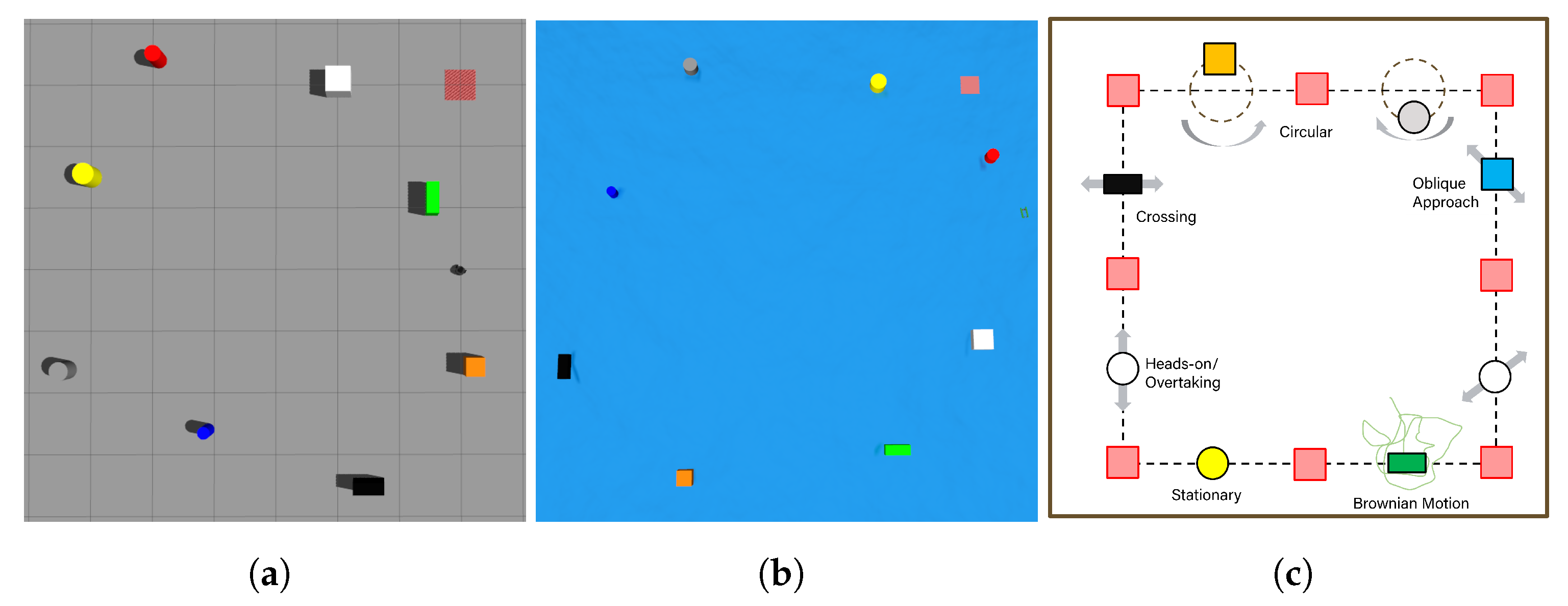
- Building training and testing simulation environments where the moving obstacles can be integrated in random order to better train the agent and better evaluate the effectiveness of the trained agent;
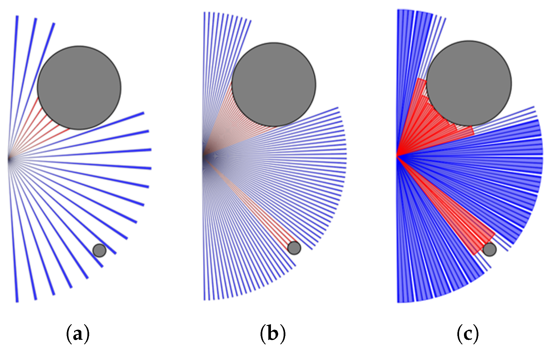
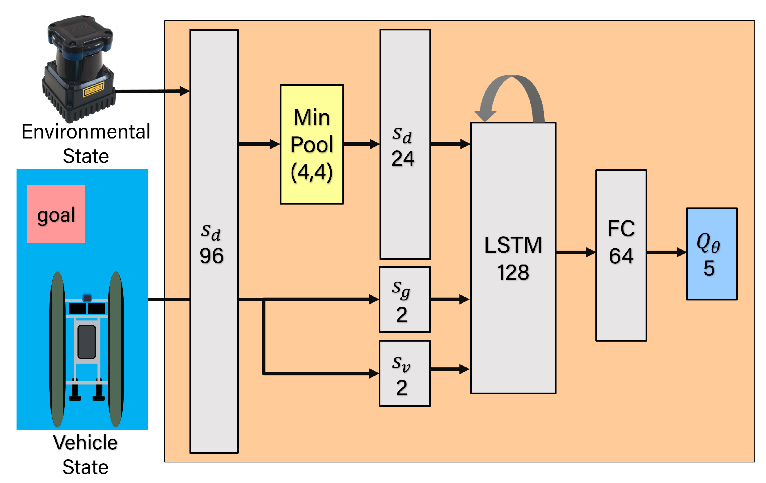
- Designing the DQN network architecture to enable the agent to avoid dynamic obstacles. Specifically, we perform min pooling on input Lidar ranges to keep high accuracy while low dimensionality. We use Long Short-Term Memory (LSTM) as a building block to process the entire sequence of data to help the agent better capture the motion of the obstacles;
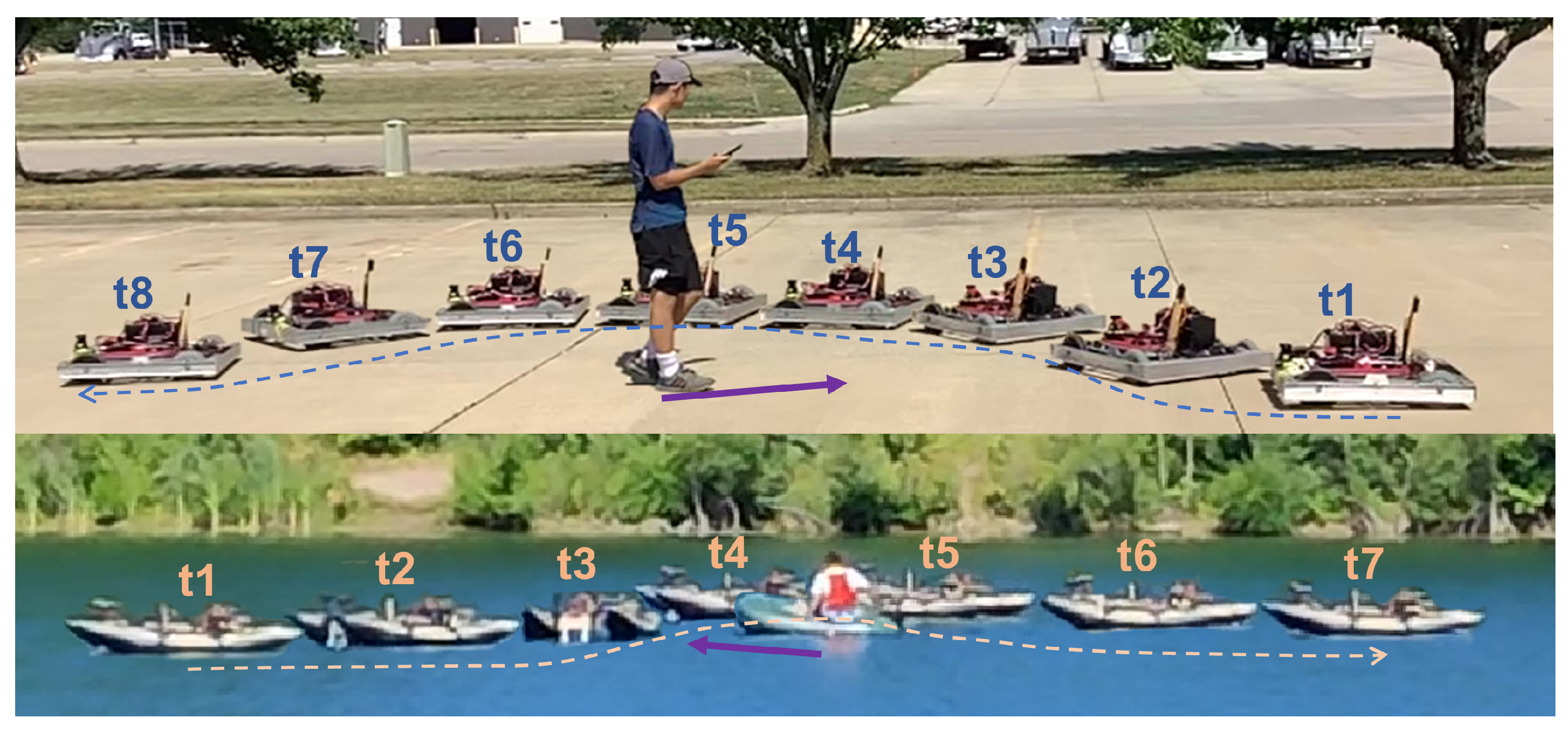
- Presenting a method that successfully enables cross-domain training and validation of a DQN across domains, moving from data-rich and accessible environments to data-poor and difficult to access environments;
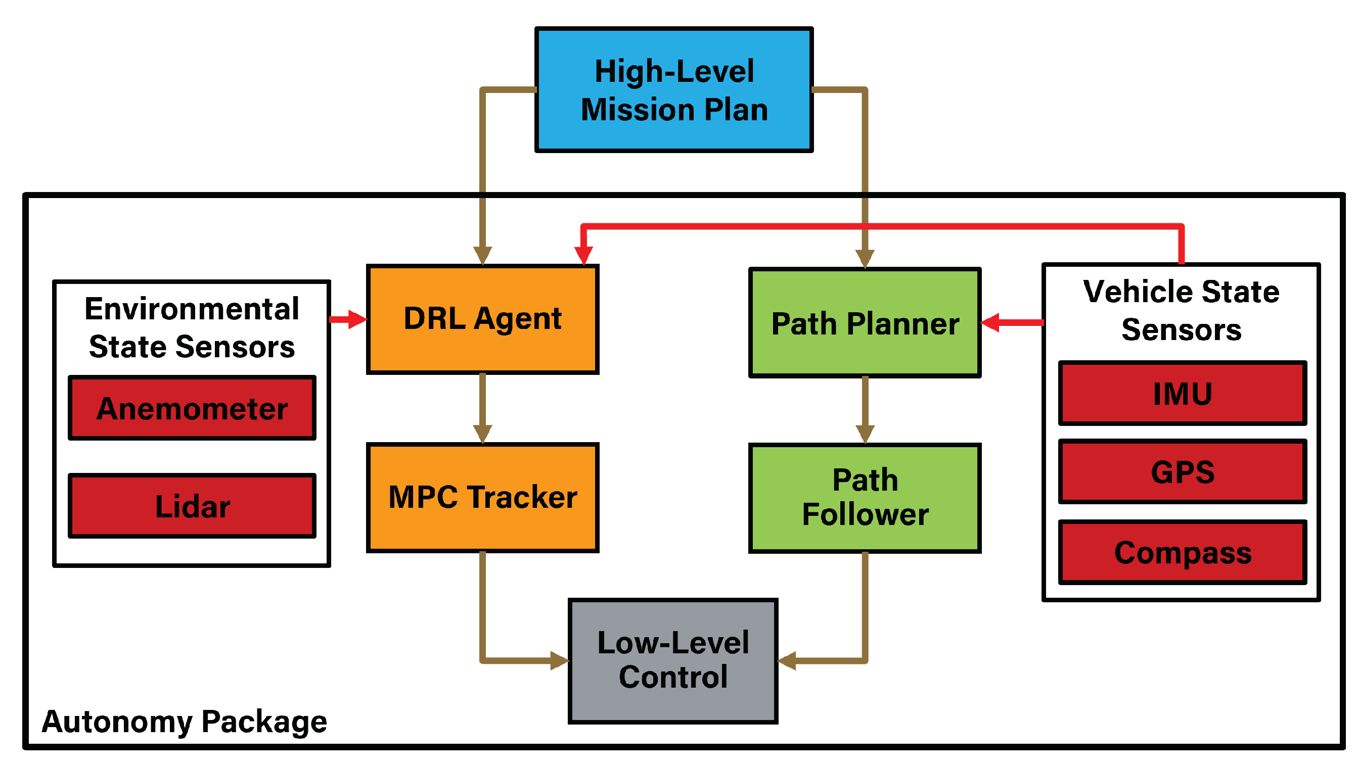
- Using a neural network to approximate the dynamics of USV system and implementing NN-MPC waypoint tracker as a low-level controller for the DRL agent to effectively avoid obstacles while rejecting disturbances that are not included during DQN training.
2. Methodology
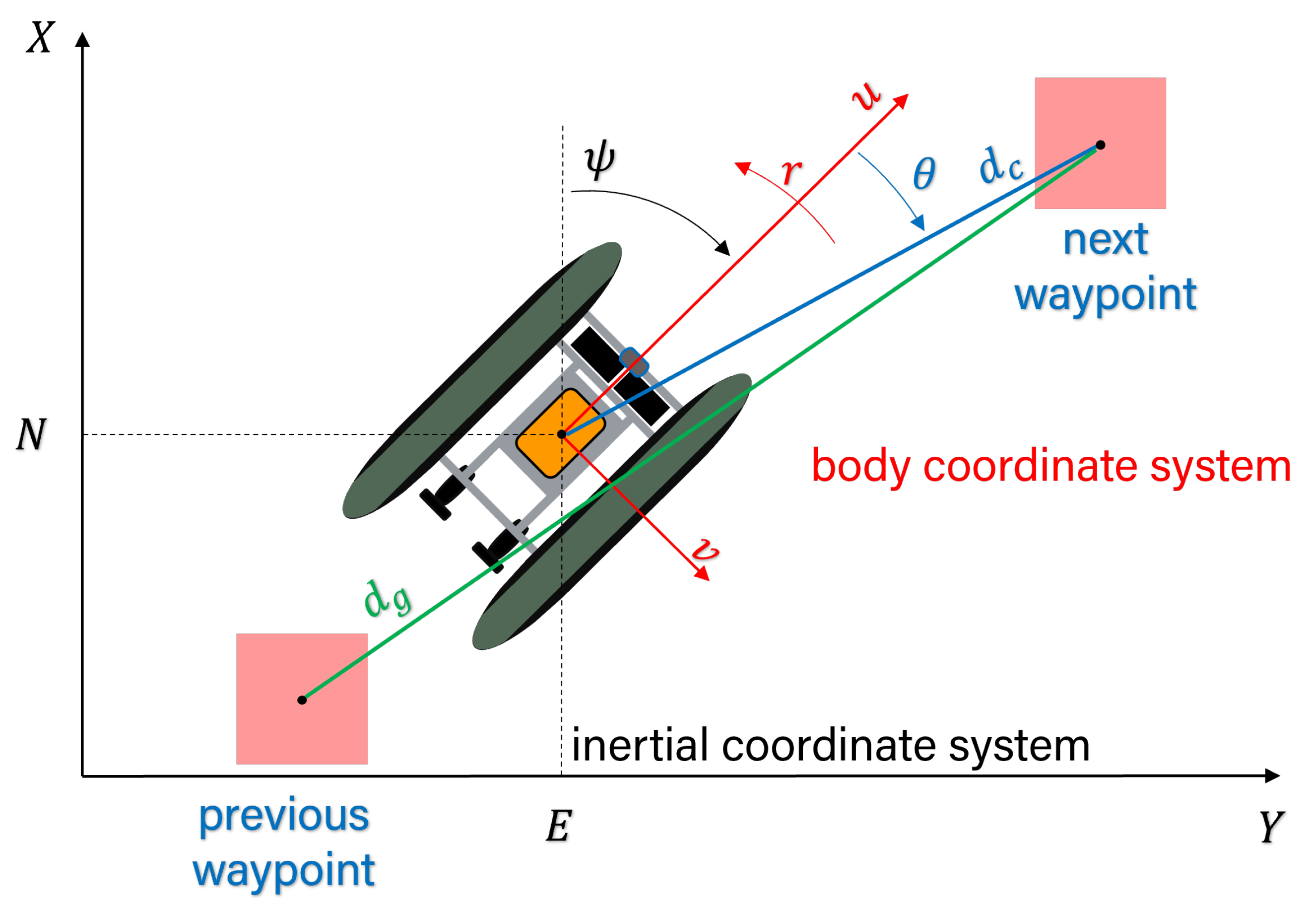
2.1. Path Planner
2.2. Path Follower
2.3. DRL Agent
2.4. NN-MPC Tracker
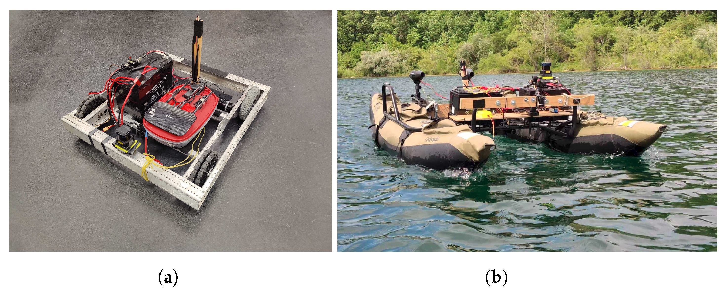
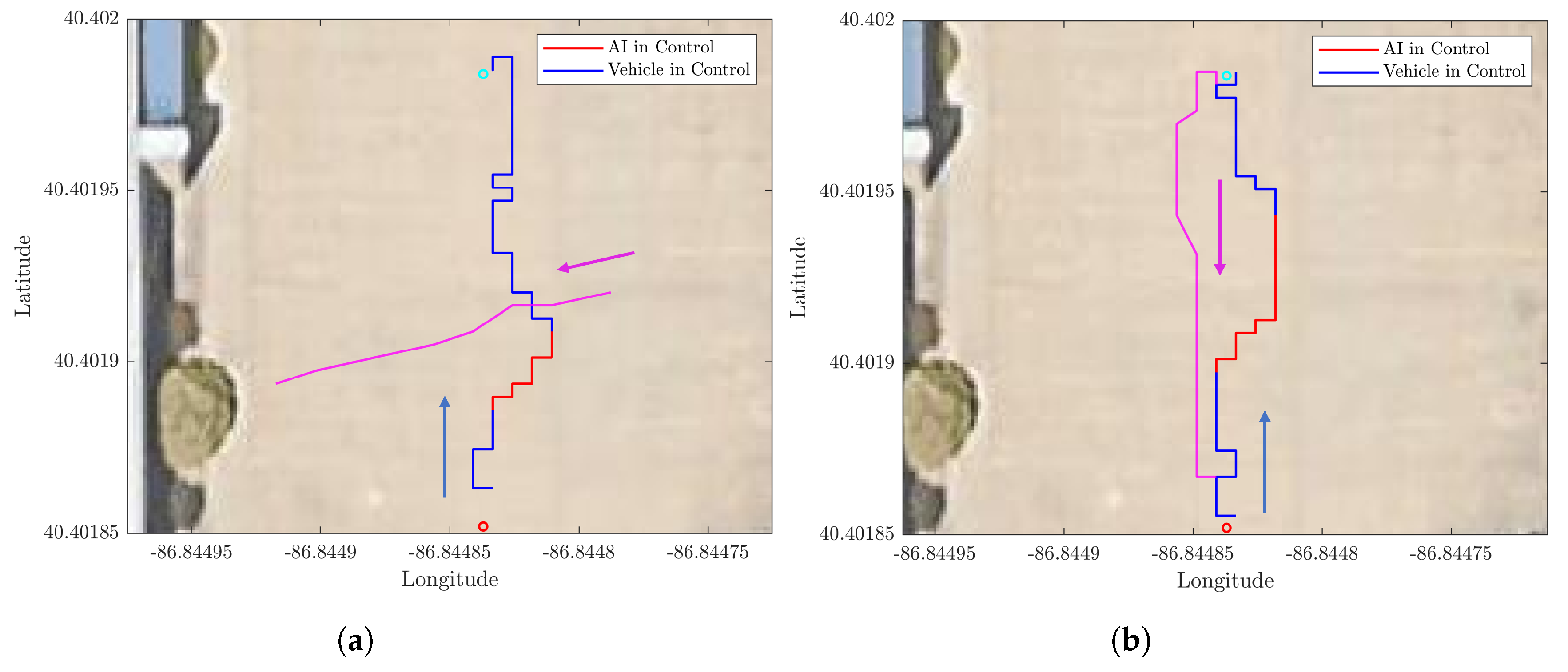
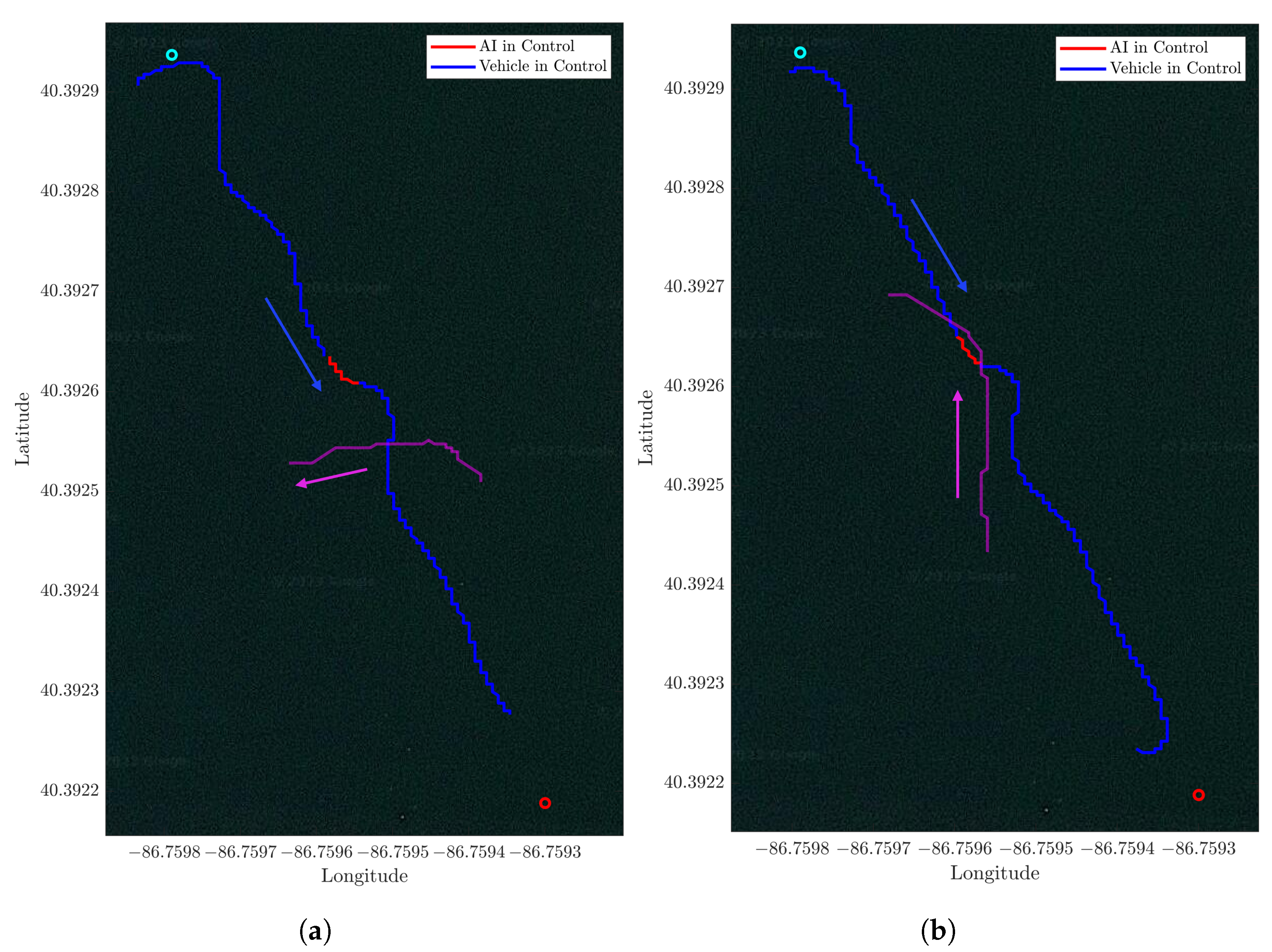
2.5. Field Test Implementation
| Algorithm 1: DRL Path Augmentation for Obstacle Avoidance |
| initialization; mission = [[initialization point], [n waypoints of type (N, E)]]; current_path = path between mission waypoints;  |
3. Results
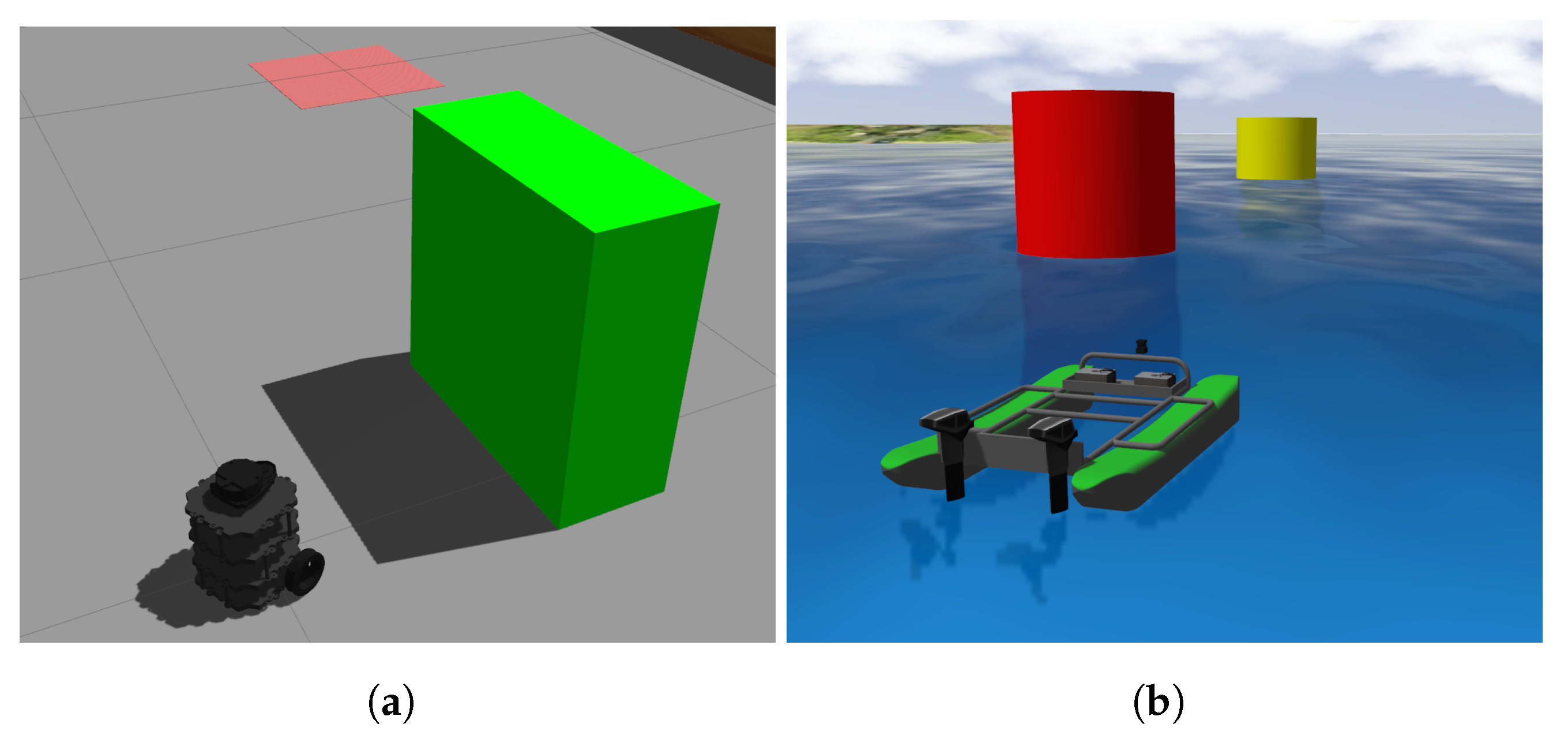
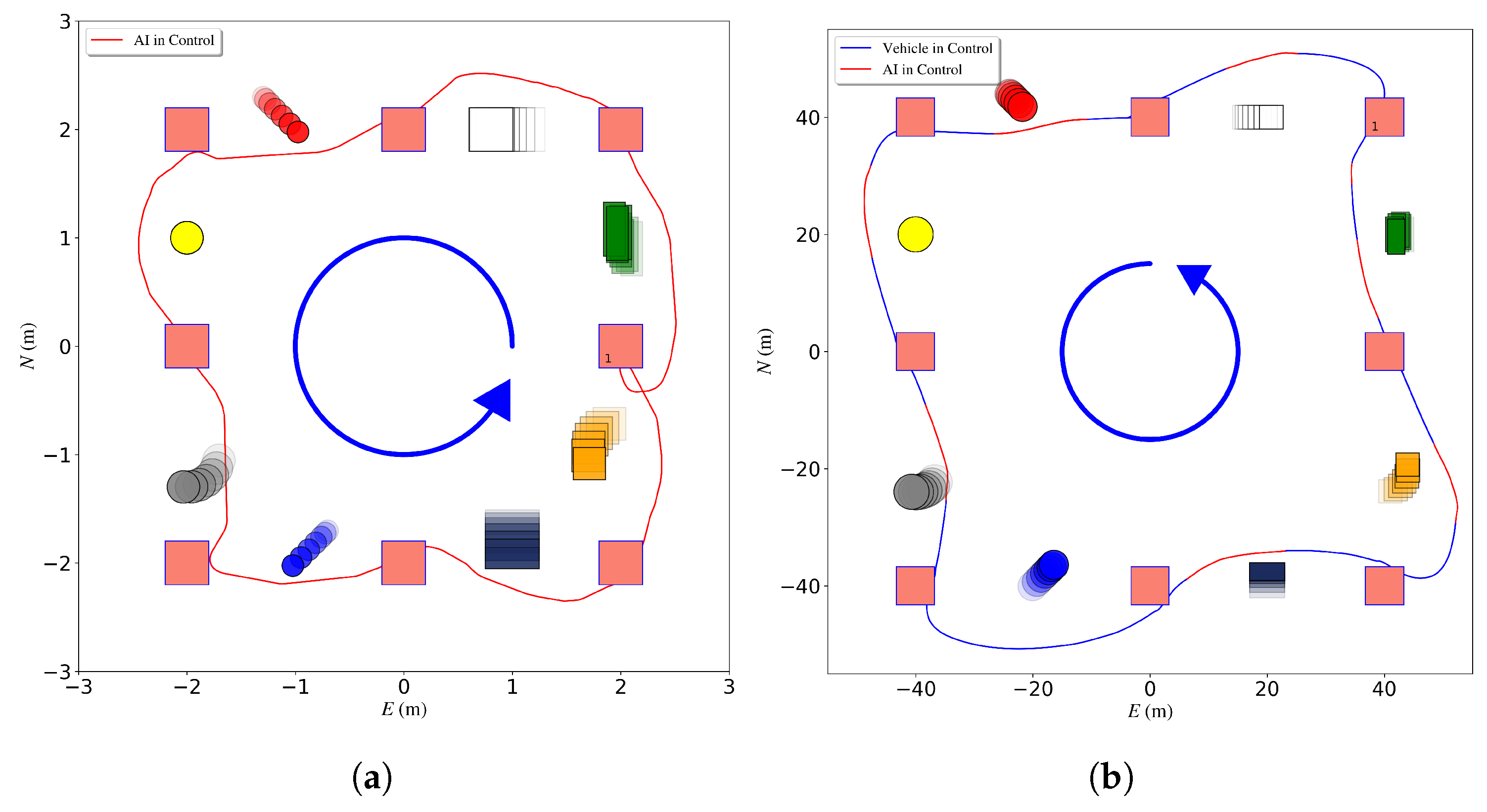
3.1. Simulation Environments
3.2. DQN Network Architecture
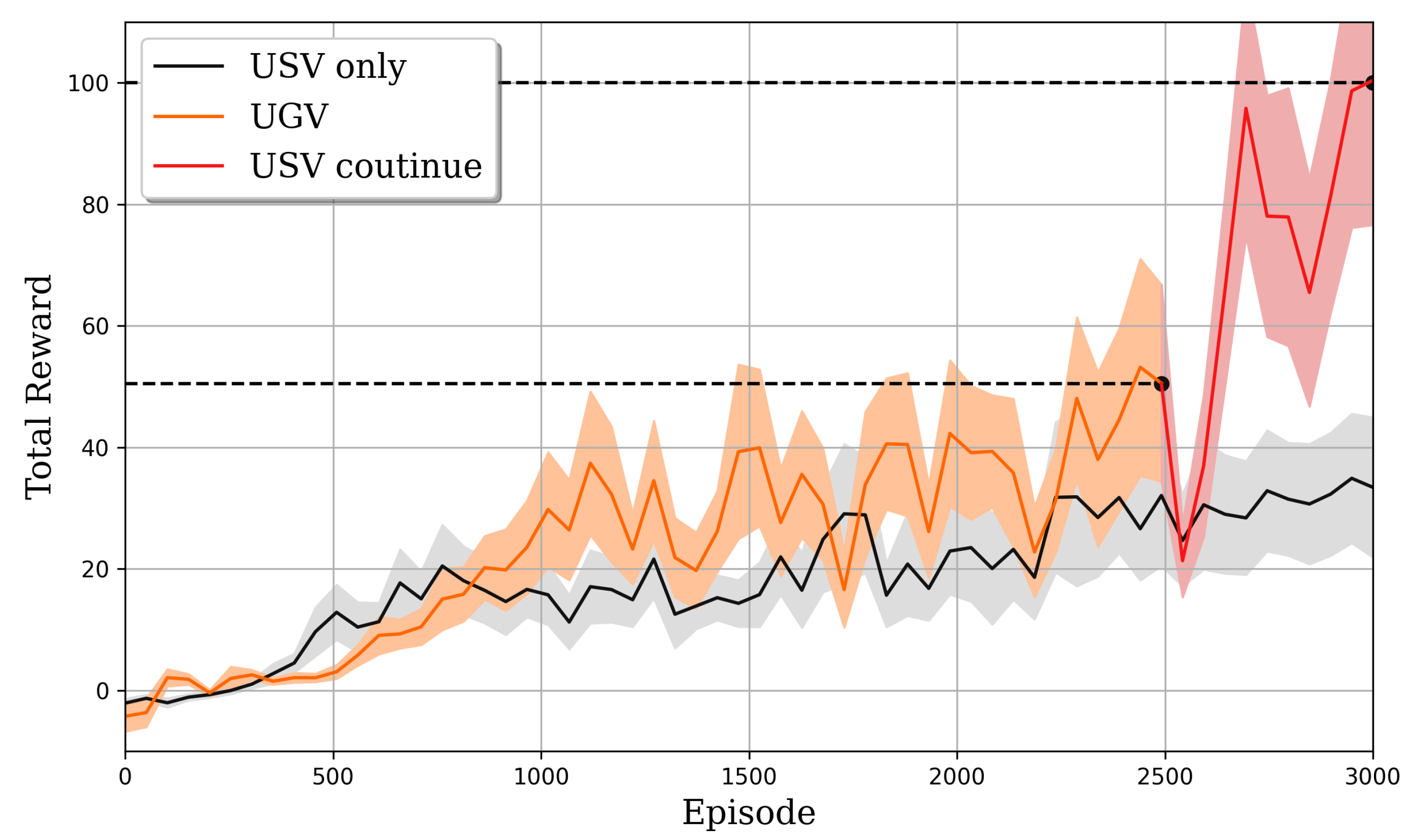
3.3. Cross Domain Training and Validation
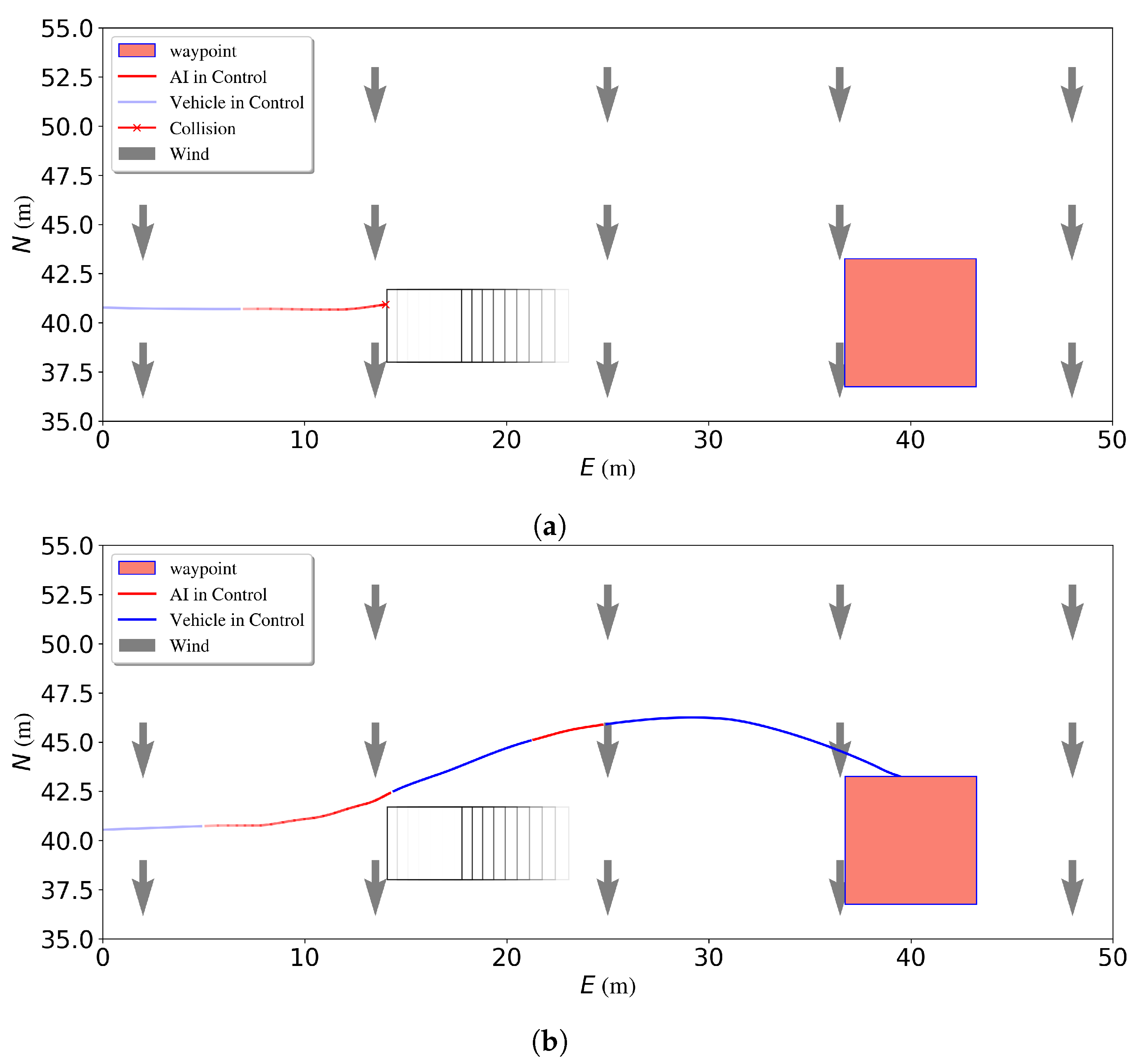
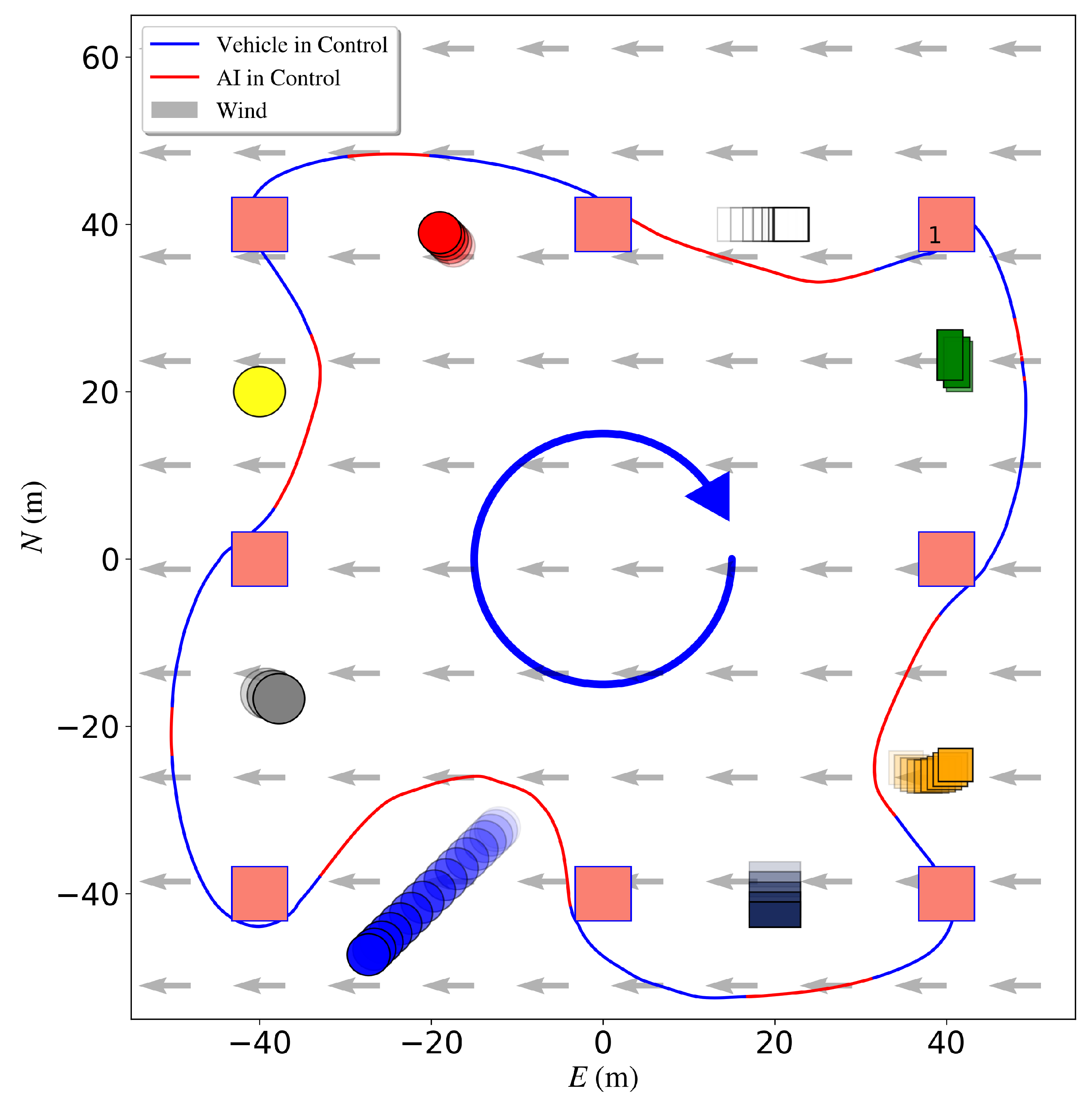
3.4. NN-MPC Waypoint Tracker
4. Conclusions
Author Contributions
Funding
Institutional Review Board Statement
Informed Consent Statement
Data Availability Statement
Acknowledgments
Conflicts of Interest
References
- Cockcroft, A.N.; Lameijer, J.N.F. Guide to the Collision Avoidance Rules; Elsevier: Amsterdam, The Netherlands, 2003. [Google Scholar]
- Vagale, A.; Oucheikh, R.; Bye, R.T.; Osen, O.L.; Fossen, T.I. Path planning and collision avoidance for autonomous surface vehicles I: A review. J. Mar. Sci. Technol. 2021, 26, 1292–1306. [Google Scholar] [CrossRef]
- Zhang, H.Y.; Lin, W.M.; Chen, A.X. Path planning for the mobile robot: A review. Symmetry 2018, 10, 450. [Google Scholar] [CrossRef] [Green Version]
- Ferguson, D.; Stentz, A. Using interpolation to improve path planning: The Field D* algorithm. J. Field Robot. 2006, 23, 79–101. [Google Scholar] [CrossRef] [Green Version]
- Sampedro, C.; Bavle, H.; Rodriguez-Ramos, A.; de La Puente, P.; Campoy, P. Laser-based reactive navigation for multirotor aerial robots using deep reinforcement learning. In Proceedings of the 2018 IEEE/RSJ International Conference on Intelligent Robots and Systems (IROS), Madrid, Spain, 1–5 October 2018; pp. 1024–1031. [Google Scholar]
- Han, J.; Cho, Y.; Kim, J.; Kim, J.; Son, N.; Kim, S.Y. Autonomous collision detection and avoidance for ARAGON USV: Development and field tests. J. Field Robot. 2020, 37, 987–1002. [Google Scholar] [CrossRef]
- Gao, Y.; Gordon, T.; Lidberg, M. Optimal control of brakes and steering for autonomous collision avoidance using modified Hamiltonian algorithm. Veh. Syst. Dyn. 2019, 57, 1224–1240. [Google Scholar] [CrossRef]
- Lindqvist, B.; Mansouri, S.S.; Agha-mohammadi, A.; Nikolakopoulos, G. Nonlinear MPC for Collision Avoidance and Control of UAVs With Dynamic Obstacles. IEEE Robot. Autom. Lett. 2020, 5, 6001–6008. [Google Scholar] [CrossRef]
- Hagen, I.B.; Kufoalor, D.K.M.; Brekke, E.F.; Johansen, T.A. MPC-based Collision Avoidance Strategy for Existing Marine Vessel Guidance Systems. In Proceedings of the 2018 IEEE International Conference on Robotics and Automation (ICRA), Brisbane, Australia, 21–25 May 2018; pp. 7618–7623. [Google Scholar] [CrossRef]
- Eriksen, B.O.H.; Breivik, M. Short-term ASV Collision Avoidance with Static and Moving Obstacles. Model. Identif. Control. A Nor. Res. Bull. 2019, 40, 177–187. [Google Scholar] [CrossRef] [Green Version]
- Zhang, X.; Wang, C.; Jiang, L.; An, L.; Yang, R. Collision-avoidance navigation systems for Maritime Autonomous Surface Ships: A state of the art survey. Ocean Eng. 2021, 235, 109380. [Google Scholar] [CrossRef]
- Mnih, V.; Kavukcuoglu, K.; Silver, D.; Rusu, A.A.; Veness, J.; Bellemare, M.G.; Graves, A.; Riedmiller, M.; Fidjeland, A.K.; Ostrovski, G.; et al. Human-level control through deep reinforcement learning. Nature 2015, 518, 529–533. [Google Scholar] [CrossRef]
- Choi, J.; Park, K.; Kim, M.; Seok, S. Deep reinforcement learning of navigation in a complex and crowded environment with a limited field of view. In Proceedings of the 2019 International Conference on Robotics and Automation (ICRA), Montreal, QC, Canada, 20–24 May 2019; pp. 5993–6000. [Google Scholar]
- Meyer, E.; Heiberg, A.; Rasheed, A.; San, O. COLREG-compliant collision avoidance for unmanned surface vehicle using deep reinforcement learning. IEEE Access 2020, 8, 165344–165364. [Google Scholar] [CrossRef]
- Xiao, X.; Liu, B.; Warnell, G.; Stone, P. Toward agile maneuvers in highly constrained spaces: Learning from hallucination. IEEE Robot. Autom. Lett. 2021, 6, 1503–1510. [Google Scholar] [CrossRef]
- Joshi, G.; Chowdhary, G. Cross-domain transfer in reinforcement learning using target apprentice. In Proceedings of the 2018 IEEE International Conference on Robotics and Automation (ICRA), Brisbane, Australia, 21–25 May 2018; pp. 7525–7532. [Google Scholar]
- Shukla, Y.; Thierauf, C.; Hosseini, R.; Tatiya, G.; Sinapov, J. ACuTE: Automatic Curriculum Transfer from Simple to Complex Environments. arXiv 2022, arXiv:2204.04823. [Google Scholar]
- Gage, D.W. UGV History 101: A Brief History of Unmanned Ground Vehicle (UGV) Development Efforts; Technical report; NAVAL COMMAND CONTROL AND OCEAN SURVEILLANCE CENTER RDT AND E DIV SAN DIEGO CA: Fort Belvoir, VA, USA, 1995. [Google Scholar]
- Liu, Z.; Zhang, Y.; Yu, X.; Yuan, C. Unmanned surface vehicles: An overview of developments and challenges. Annu. Rev. Control 2016, 41, 71–93. [Google Scholar] [CrossRef]
- Fossen, T.I. Handbook of Marine Craft Hydrodynamics and Motion Control; John Wiley & Sons: Hoboken, NJ, USA, 2011. [Google Scholar]
- Lambert, R.; Li, J.; Wu, L.F.; Mahmoudian, N. Robust ASV Navigation Through Ground to Water Cross-Domain Deep Reinforcement Learning. Front. Robot. AI 2021, 8, 739023. [Google Scholar] [CrossRef] [PubMed]
- Fossen, T.I.; Pettersen, K.Y.; Galeazzi, R. Line-of-Sight Path Following for Dubins Paths With Adaptive Sideslip Compensation of Drift Forces. IEEE Trans. Control Syst. Technol. 2015, 23, 820–827. [Google Scholar] [CrossRef] [Green Version]
- Dubins, L.E. On curves of minimal length with a constraint on average curvature, and with prescribed initial and terminal positions and tangents. Am. J. Math. 1957, 79, 497–516. [Google Scholar] [CrossRef]
- Caharija, W. Integral line-of-sight guidance and control of underactuated marine vehicles. IEEE Trans. Control. Syst. Technol. 2014, 24, 1–20. [Google Scholar]
- Sutton, R.S.; Barto, A.G. Reinforcement Learning: An Introduction; MIT Press: Cambridge, MA, USA, 2018. [Google Scholar]
- Hochreiter, S.; Schmidhuber, J. Long Short-Term Memory. Neural Comput. 1997, 9, 1735–1780. [Google Scholar] [CrossRef]
- Lambert, R.; Page, B.; Chavez, J.; Mahmoudian, N. A Low-Cost Autonomous Surface Vehicle for Multi-Vehicle Operations. In Proceedings of the Global Oceans 2020: Singapore–US Gulf Coast, Biloxi, MI, USA, 5–30 October 2020; pp. 1–5. [Google Scholar]
- Forgione, M.; Piga, D. Continuous-time system identification with neural networks: Model structures and fitting criteria. Eur. J. Control 2021, 59, 69–81. [Google Scholar] [CrossRef]
- Quigley, M.; Conley, K.; Gerkey, B.; Faust, J.; Foote, T.; Leibs, J.; Berger, E.; Wheeler, R.; Ng, A.Y. ROS: An open-source Robot Operating System. In Proceedings of the ICRA Workshop on Open Source Software, Kobe, Japan, 12–17 May 2009; Volume 3, p. 5. [Google Scholar]
- Hokuyo Automatic Co., Ltd. Hokuyo UTM-30LX-EW Scanning Laser Rangefinder. Available online: https://acroname.com/store/scanning-laser-rangefinder-r354-utm-30lx-ew (accessed on 9 March 2023).
- Bingham, B.; Aguero, C.; McCarrin, M.; Klamo, J.; Malia, J.; Allen, K.; Lum, T.; Rawson, M.; Waqar, R. Toward Maritime Robotic Simulation in Gazebo. In Proceedings of the MTS/IEEE OCEANS Conference, Seattle, WA, USA, 27–31 October 2019. [Google Scholar]
- Bujarbaruah, M.; Zhang, X.; Tanaskovic, M.; Borrelli, F. Adaptive stochastic MPC under time-varying uncertainty. IEEE Trans. Autom. Control 2020, 66, 2840–2845. [Google Scholar] [CrossRef]
- Ferreau, H.J.; Bock, H.G.; Diehl, M. An online active set strategy to overcome the limitations of explicit MPC. Int. J. Robust Nonlinear Control. IFAC-Affil. J. 2008, 18, 816–830. [Google Scholar] [CrossRef]


Disclaimer/Publisher’s Note: The statements, opinions and data contained in all publications are solely those of the individual author(s) and contributor(s) and not of MDPI and/or the editor(s). MDPI and/or the editor(s) disclaim responsibility for any injury to people or property resulting from any ideas, methods, instructions or products referred to in the content. |
© 2023 by the authors. Licensee MDPI, Basel, Switzerland. This article is an open access article distributed under the terms and conditions of the Creative Commons Attribution (CC BY) license (https://creativecommons.org/licenses/by/4.0/).
Share and Cite
Li, J.; Chavez-Galaviz, J.; Azizzadenesheli, K.; Mahmoudian, N. Dynamic Obstacle Avoidance for USVs Using Cross-Domain Deep Reinforcement Learning and Neural Network Model Predictive Controller. Sensors 2023, 23, 3572. https://doi.org/10.3390/s23073572
Li J, Chavez-Galaviz J, Azizzadenesheli K, Mahmoudian N. Dynamic Obstacle Avoidance for USVs Using Cross-Domain Deep Reinforcement Learning and Neural Network Model Predictive Controller. Sensors. 2023; 23(7):3572. https://doi.org/10.3390/s23073572
Chicago/Turabian StyleLi, Jianwen, Jalil Chavez-Galaviz, Kamyar Azizzadenesheli, and Nina Mahmoudian. 2023. "Dynamic Obstacle Avoidance for USVs Using Cross-Domain Deep Reinforcement Learning and Neural Network Model Predictive Controller" Sensors 23, no. 7: 3572. https://doi.org/10.3390/s23073572