
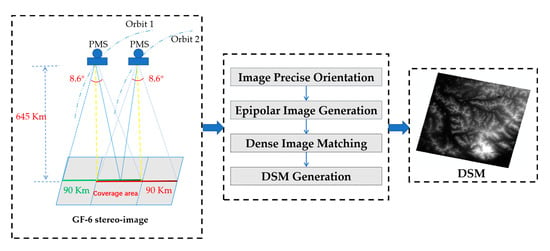
DSM Extraction Based on Gaofen-6 Satellite High-Resolution Cross-Track Images with Wide Field of View
Abstract
:
1. Introduction
2. Materials and Methods
2.1. Accurate Orientation of Stereo Images Based on an Error-Compensated RPCs Model
2.2. Epipolar Image Generation Based on the Projection Trajectory Method
2.3. Dense Image Matching
2.3.1. Pre-Processing of Image
2.3.2. Calculation of Cost
2.3.3. Dynamic Planning
2.3.4. Post-Processing of Disparity Map
2.4. DSM Generation
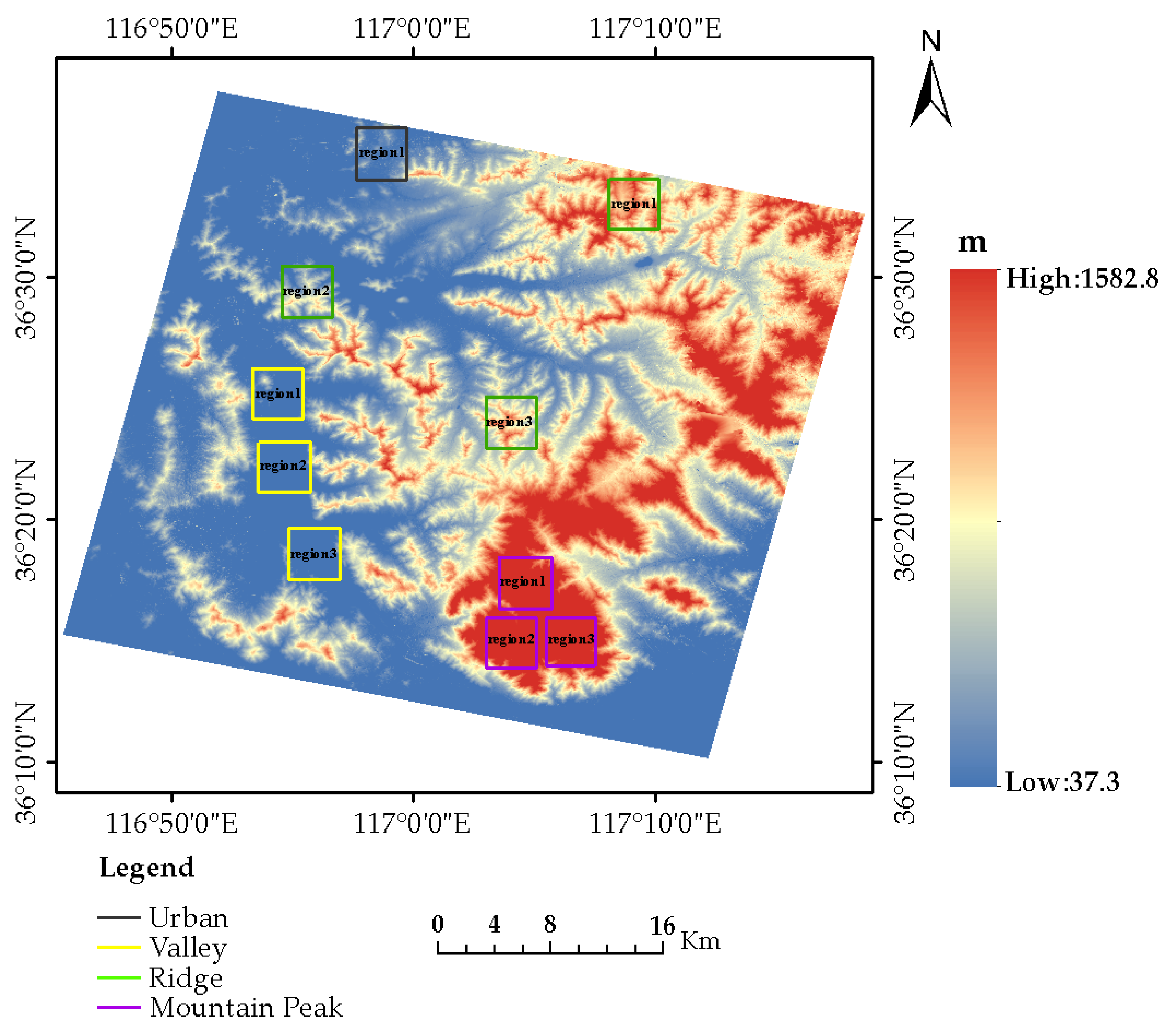
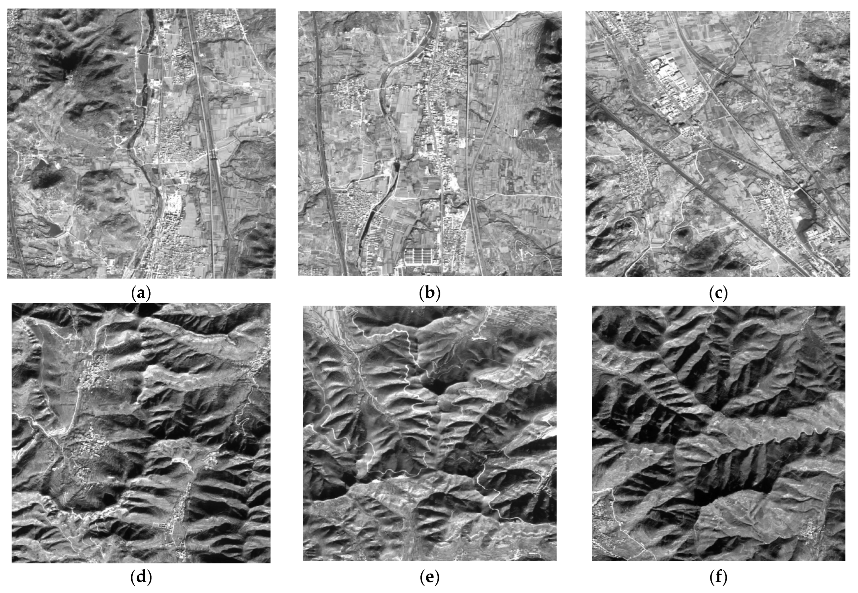
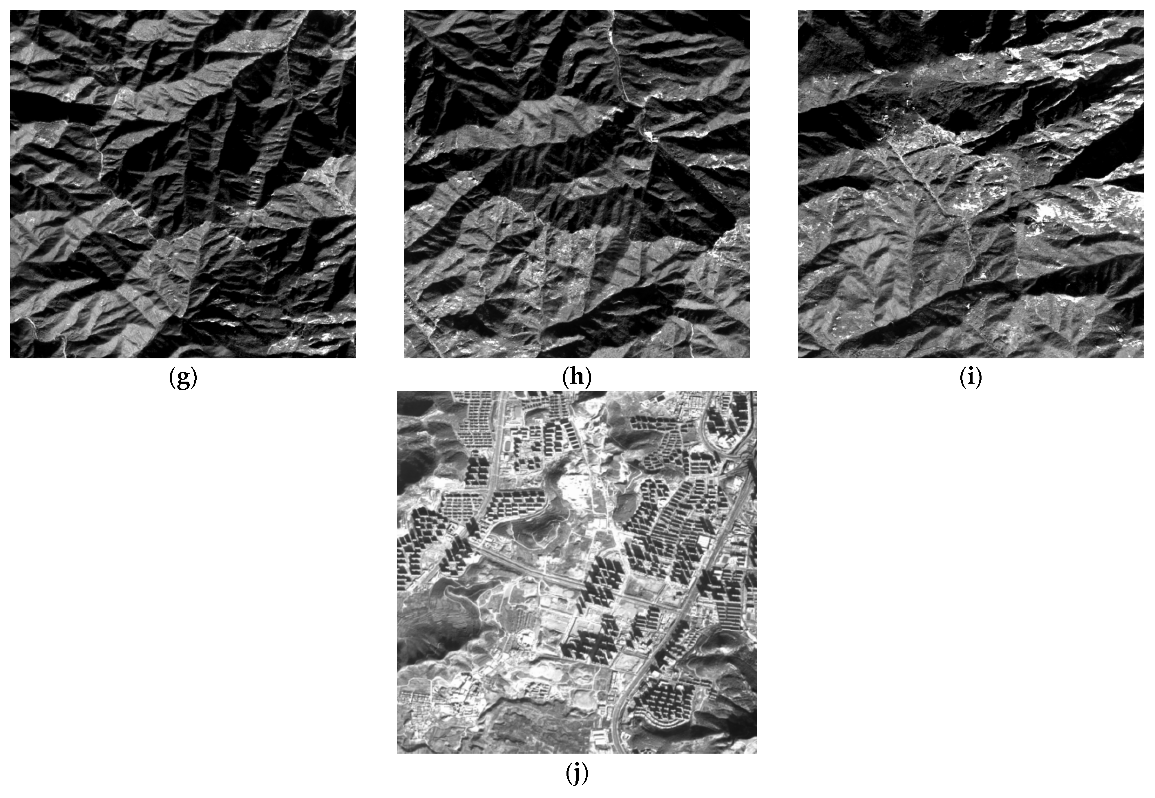
2.5. Experimental Data
3. Experiment Results and Analysis
3.1. Orientation Results
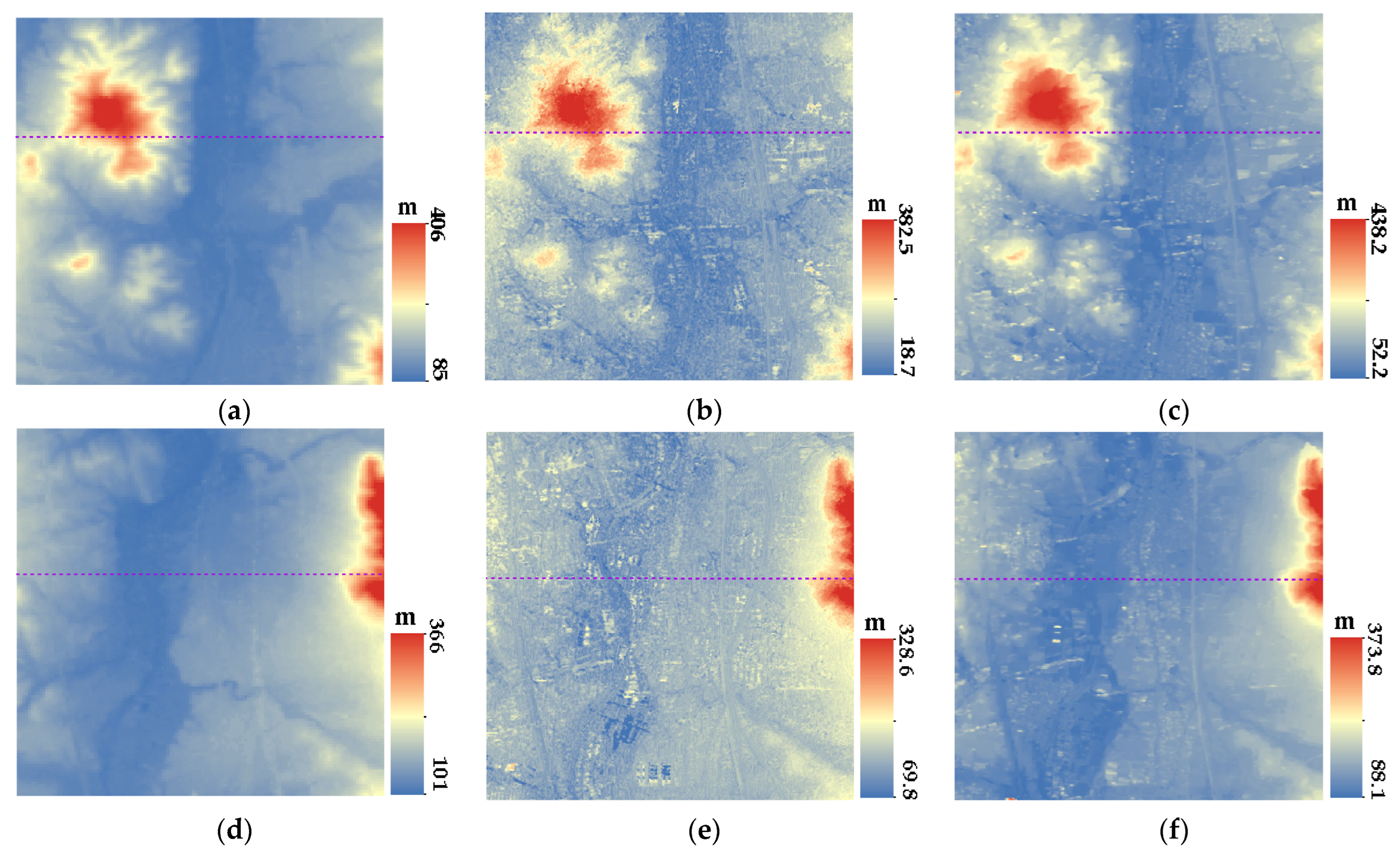
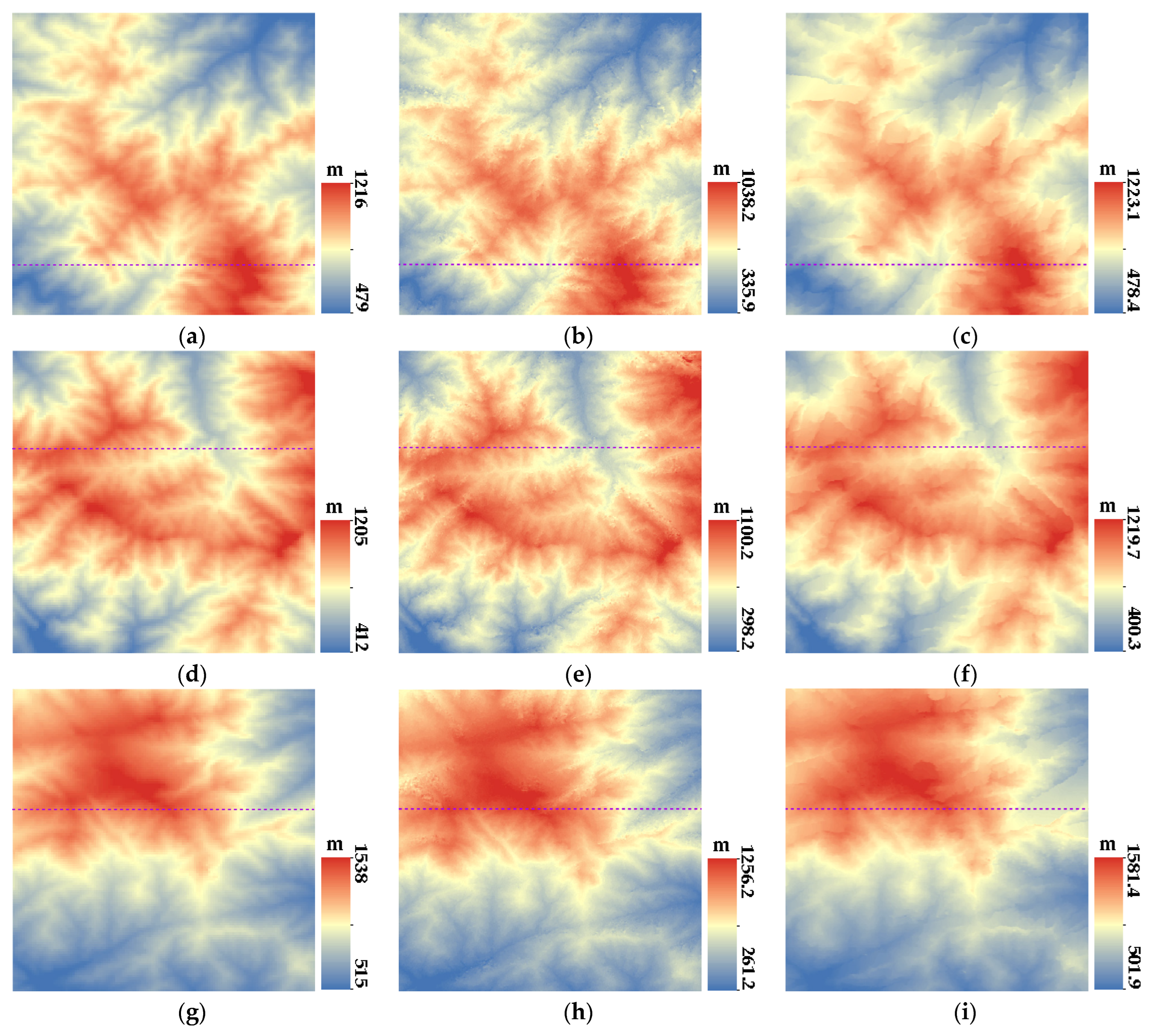
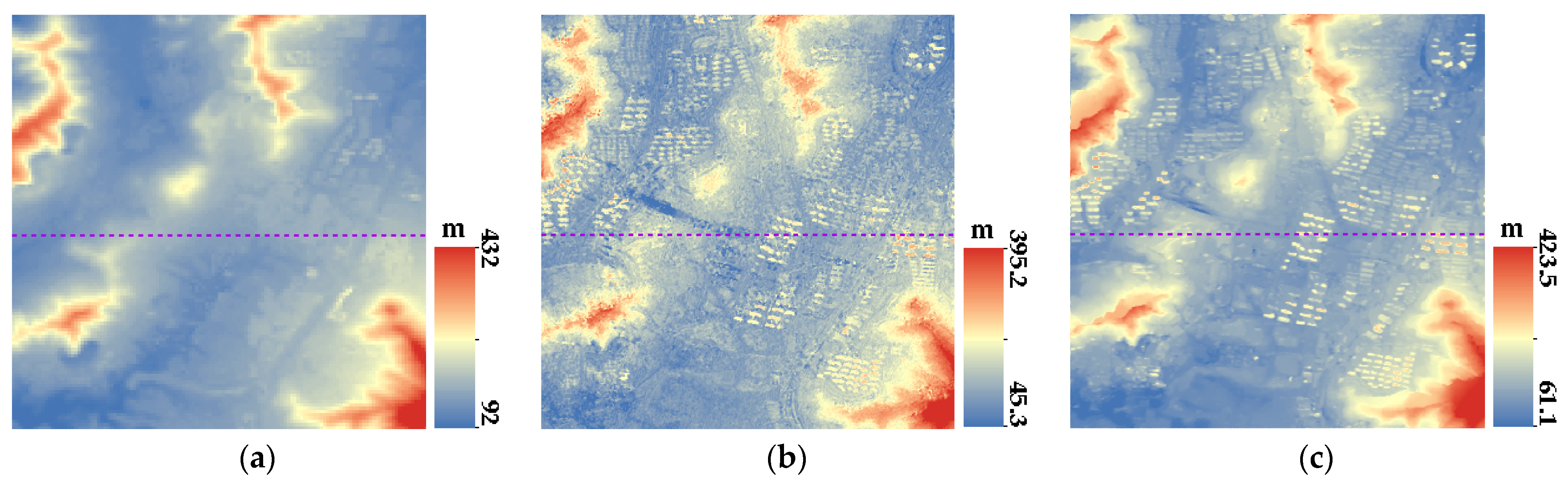
3.2. DSM Results
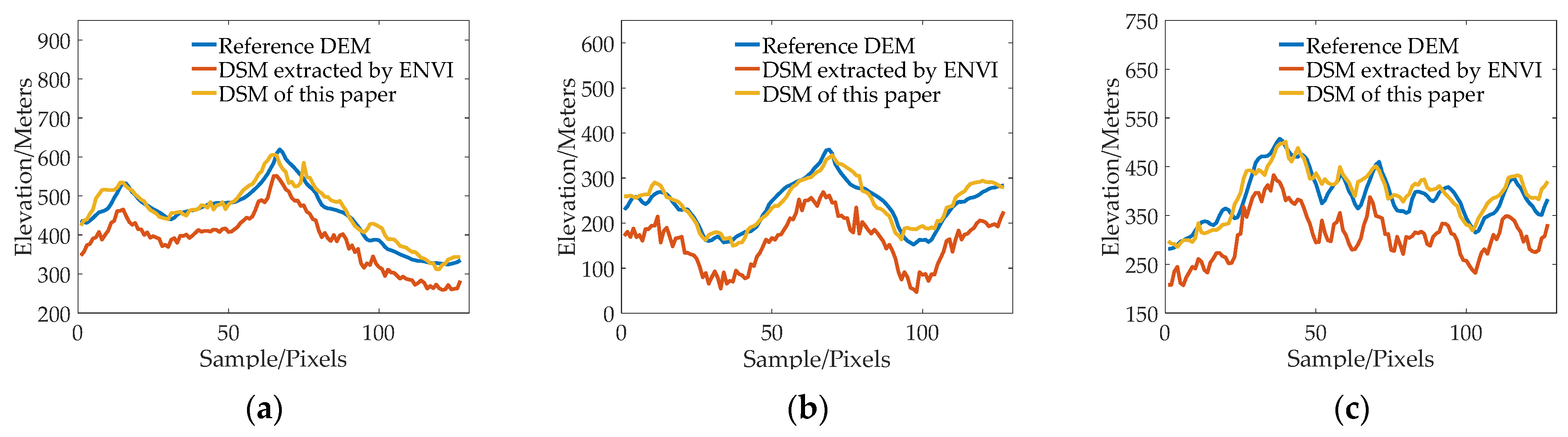
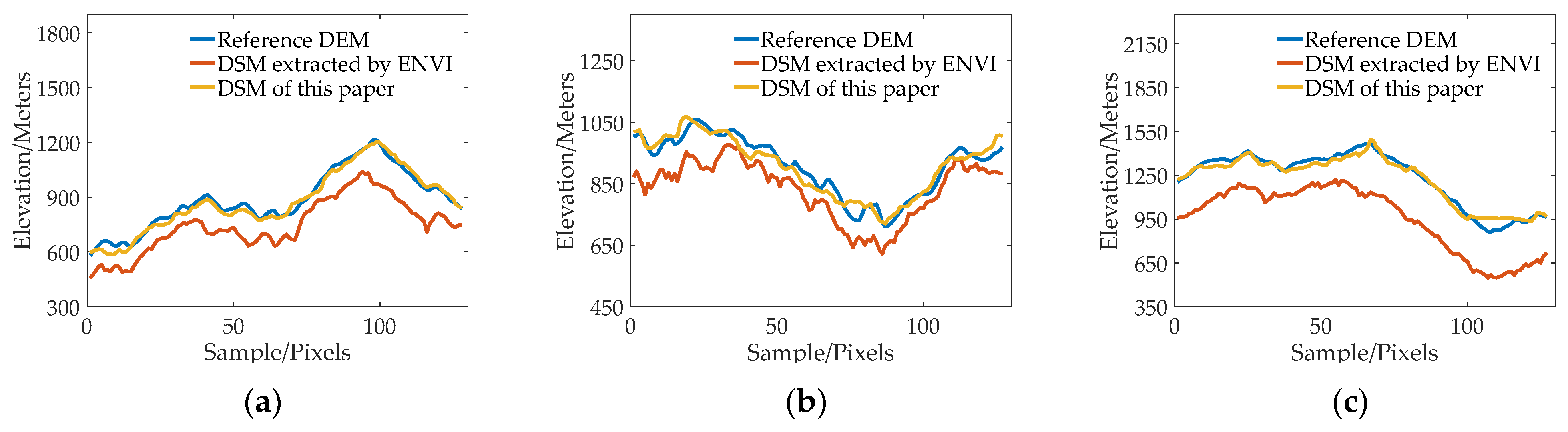
3.3. DSM Accuracy Analysis
4. Conclusions
Author Contributions
Funding
Institutional Review Board Statement
Informed Consent Statement
Data Availability Statement
Acknowledgments
Conflicts of Interest
References
- Martha, T.R.; Kerle, N.; Jetten, V.; van Westen, C.J.; Kumar, K.V. Characterising spectral, spatial and morphometric properties of landslides for semi-automatic detection using object-oriented methods. Geomorphology 2010, 116, 24–36. [Google Scholar] [CrossRef]
- Boulton, S.J.; Martin, S. Which DEM is best for analyzing fluvial landscape development in mountainous terrains? Geomorphology 2018, 310, 168–187. [Google Scholar] [CrossRef]
- Wang, Y.P.; Dong, P.L.; Liao, S.B.; Zhu, Y.Q. Urban Expansion Monitoring Based on the Digital Surface Model—A Case Study of the Beijing–Tianjin–Hebei Plain. Appl. Sci. 2022, 12, 5312. [Google Scholar] [CrossRef]
- Zhu, X.Y.; Tang, X.M.; Zhang, G.; Liu, B.; Hu, W.M. Accuracy Comparison and Assessment of DSM Derived from GFDM Satellite and GF-7 Satellite Imagery. Remote Sens. 2021, 13, 4791. [Google Scholar] [CrossRef]
- Gindraux, S.; Boesch, R.; Farinotti, D. Accuracy assessment of digital surface models from unmanned aerial vehicles’ imagery on glaciers. Remote Sens. 2017, 9, 186. [Google Scholar] [CrossRef] [Green Version]
- Mo, F.; Cao, H.Y.; Liu, X.W.; Gao, H.T.; Huang, Y. Research on Space Mapping System with Large Scale. Spacecr. Eng. 2017, 26, 12–19. [Google Scholar]
- Bouillon, A.; Bernard, M.; Gigord, P.; Orsoni, A.; Rudowski, V.; Baudoin, A. SPOT 5 HRS Geometric Performance: Using Block Adjustment as a Key Issue to Improve Quality of DEM Generation. ISPRS J. Photogramm. Remote Sens. 2006, 60, 134–146. [Google Scholar] [CrossRef]
- Toutin, T. Generation of DSMs from SPOT-5 in-track HRS and across-track HRG stereo data using spatiotriangulation and autocalibration. ISPRS J. Photogramm. Remote Sens. 2006, 60, 170–181. [Google Scholar] [CrossRef]
- Zhao, L.P.; Liu, F.D.; Li, J.; Wang, W. Preliminary Research on Position Accuracy of IRS-P5. Remote Sens. Inf. 2007, 2, 28–32. [Google Scholar]
- d’Angelo, P.; Uttenthaler, A.; Carl, S.; Barner, F.; Reinartz, P. Automatic generation of high quality DSM Based on IRS-P5 Cartosat-1 Stereo Data. In Proceedings of the ESA Living Planet Symposium, Bergen, Norway, 28 June–2 July 2010; Special Publication SP-686. pp. 1–5. [Google Scholar]
- Cao, H.Y.; Zhang, X.W.; Zhao, C.G.; Xu, C.; Mo, F.; Dai, J. System design and key technology of the GF-7 satellite. Chin. Space Sci. Technol. 2020, 40, 1–9. [Google Scholar]
- Li, D.R.; Wang, M. A Review of High Resolution Optical Satellite Surveying and Mapping Technology. Spacecr. Recovery Remote Sens. 2020, 41, 1–11. [Google Scholar]
- Rosenqvist, A.; Shimada, M.; Ito, N.; Watanabe, M. ALOS PALSAR: A pathfinder mission for global-scale monitoring of the environment. IEEE Trans. Geosci. Remote Sens. 2007, 45, 3307–3316. [Google Scholar] [CrossRef]
- Ni, W.J.; Guo, Z.F.; Zhang, Z.Y.; Sun, G.Q.; Huang, W.L. Semi-automatic extraction of digital surface model using ALOS/PRISM data with ENVI. In Proceedings of the Geoscience & Remote Sensing Symposium, Munich, Germany, 12 November 2012. [Google Scholar]
- Takaku, J.; Tadono, T.; Tsutsui, K. Generation of High Resolution Global DSM from ALOS PRISM. ISPRS Ann. Photogramm. Remote Sens. Spat. Inf. Sci. 2014, 2, 243–248. [Google Scholar] [CrossRef] [Green Version]
- Wang, T.Y.; Zhang, G.; Li, D.R.; Tang, X.M.; Jiang, Y.H.; Pan, H.B.; Zhu, X.Y.; Fang, C. Geometric accuracy validation for ZY-3 satellite imagery. IEEE Geosci. Remote Sens. Lett. 2013, 11, 1168–1171. [Google Scholar] [CrossRef]
- Li, D.R. China’s First Civilian Three-line-array Stereo Mapping Satellite: ZY-3. Acta Geod. Et Cartogr. Sin. 2012, 41, 317–322. [Google Scholar]
- Tang, X.M.; Zhang, G.; Zhu, X.Y.; Pan, H.B.; Jiang, Y.H.; Zhou, P.; Wang, X. Triple linear-array image geometry model of ZiYuan-3 surveying satellite and its validation. Int. J. Image Data Fusion 2013, 4, 33–51. [Google Scholar] [CrossRef]
- Eckert, S. Validation of aircraft height extraction from Worldview-1 stereo data. Int. J. Remote Sens. 2009, 30, 6053–6060. [Google Scholar] [CrossRef]
- Aguilar, M.A.; Nemmaoui, A.; Aguilar, F.J.; Qin, R.J. Quality assessment of digital surface models extracted from WorldView-2 and WorldView-3 stereo pairs over different land covers. GIScience Remote Sens. 2019, 56, 109–129. [Google Scholar] [CrossRef] [Green Version]
- Feng, Z.K.; Shi, D.; Chen, W.X.; Luo, A.R. The Progress of French Remote Sensing Satellite-from SPOT Toward Pleiades. Remote Sens. Inf. 2007, 4, 87–92. [Google Scholar]
- Aguilar, M.A.; Aguilar, F.J.; Mar, S.; María, D.; Fernández, I. Geopositioning accuracy assessment of GeoEye-1 panchromatic and multispectral imagery. Photogramm. Eng. Remote Sens. 2012, 78, 247–257. [Google Scholar] [CrossRef]
- Capaldo, P.; Crespi, M.; Fratarcangeli, F.; Pieralice, F.; Nascetti, A. DSM generation from high resolution imagery: Applications with WorldView-1 and Geoeye-1. Ital. J. Remote Sens. 2012, 44, 41–53. [Google Scholar] [CrossRef]
- Hobi, M.L.; Ginzler, C. Accuracy assessment of digital surface models based on WorldView-2 and ADS80 stereo remote sensing data. Sensors 2012, 12, 6347–6368. [Google Scholar] [CrossRef] [PubMed] [Green Version]
- Aguilar, M.Á.; del Mar Saldaña, M.; Aguilar, F.J. Generation and quality assessment of stereo-extracted DSM from GeoEye-1 and WorldView-2 imagery. IEEE Trans. Geosci. Remote Sens. 2013, 52, 1259–1271. [Google Scholar] [CrossRef]
- Panagiotakis, E.; Chrysoulakis, N.; Charalampopoulou, V.; Poursanidis, D. Validation of Pleiades Tri-Stereo DSM in urban areas. ISPRS Int. J. Geo-Inf. 2018, 7, 118. [Google Scholar] [CrossRef] [Green Version]
- Zhang, L.; Gruen, A. Multi-image matching for DSM generation from IKONOS imagery. ISPRS J. Photogramm. Remote Sens. 2006, 60, 195–211. [Google Scholar] [CrossRef]
- Toutin, T. DSM generation and evaluation from QuickBird stereo imagery with 3D physical modelling. Int. J. Remote Sens. 2004, 25, 5181–5192. [Google Scholar] [CrossRef]
- Zhong, X.; Bao, S.Z. Application Advantages of Staring Area Imaging Technology (SAIT) for Microsatellites. Aerosp. China 2019, 20, 30–41. [Google Scholar]
- Bhushan, S.; Shean, D.; Alexandrov, O.; Henderson, S. Automated digital elevation model (DEM) generation from very-high-resolution Planet SkySat triplet stereo and video imagery. ISPRS J. Photogramm. Remote Sens. 2021, 173, 151–165. [Google Scholar] [CrossRef]
- Chen, S.B.; Liu, J.B.; Huang, W.C.; Chen, R.Z. Wide Swath Stereo Mapping from Gaofen-1 Wide-Field-View (WFV) Images Using Calibration. Sensors 2018, 18, 739. [Google Scholar] [CrossRef] [Green Version]
- Zhang, X.Y.; Fan, J.R.; Zhou, J.; Gui, L.H.; Bi, Y.Q. Mapping Fire Severity in Southwest China Using the Combination of Sentinel 2 and GF Series Satellite Images. Sensors 2023, 23, 2492. [Google Scholar] [CrossRef]
- Lu, C.L.; Bai, Z.G.; Li, Y.C.; Wu, B.; Qiu, G.D.; Dou, Y.F. Technical Characteristic and New Mode Applications of GF-6 Satellite. Spacecr. Eng. 2021, 30, 7–14. [Google Scholar]
- Hirschmuller, H. Stereo processing by semiglobal matching and mutual information. IEEE Trans. Pattern Anal. Mach. Intell. 2007, 30, 328–341. [Google Scholar] [CrossRef] [PubMed]
- Huang, X.; Han, Y.L.; Hu, K. An improved semi-global matching method with optimized matching aggregation constraint. IOP Conf. Ser. Earth Environ. Sci. 2020, 569, 012050. [Google Scholar] [CrossRef]
- Zhao, C.X.; Zhang, X.L.; Yang, Y. 3D reconstruction based on SGBM semi-global stereo matching algorithm. Laser J. 2021, 42, 139–143. [Google Scholar]
- Yuan, X.X.; Yuan, W.; Xu, S.; Ji, Y.H. Research developments and prospects on dense image matching in photogrammetry. Acta Geod. Et Cartogr. Sin. 2019, 48, 1542. [Google Scholar]
- Yuan, X.X.; Cao, J.S. Theory and Method of Precise Object Positioning of High Resolution Satellite Imagery; Science Press: Beijing, China, 2012; pp. 159–174. [Google Scholar]
- Tong, X.H.; Liu, S.J.; Weng, Q.H. Bias-corrected rational polynomial coefficients for high accuracy geo-positioning of QuickBird stereo imagery. ISPRS J. Photogramm. Remote Sens. 2010, 65, 218–226. [Google Scholar] [CrossRef]
- Fraser, C.S.; Hanley, H.B. Bias-compensated RPCs for sensor orientation of high-resolution satellite imagery. Photogramm. Eng. Remote Sens. 2005, 71, 909–915. [Google Scholar] [CrossRef]
- Aguilar, M.A.; Jiménez-Lao, R.; Nemmaoui, A.; Aguilar, M.A. Geometric Accuracy Assessment of Deimos-2 Panchromatic Stereo Pairs: Sensor Orientation and Digital Surface Model Production. Sensors 2020, 20, 7234. [Google Scholar] [CrossRef]
- Fraser, C.S.; Yamakawa, T. Insights into the affine model for high-resolution satellite sensor orientation. ISPRS J. Photogramm. Remote Sens. 2004, 58, 275–288. [Google Scholar] [CrossRef]
- Li, D.R.; Zhang, G.; Jiang, W.S.; Yuan, X.X. SPOT-5 HRS Satellite Imagery Block Adjustment Without GCPS or with Single GCP. Geomat. Inf. Sci. Wuhan Univ. 2006, 31, 377–381. [Google Scholar]
- Zhang, Y.J.; Ding, Y.Z. Approximate Epipolar Image Generation of Liner Array Satellite Stereos with Rational Polynomial Coefficients. Geomat. Inf. Sci. Wuhan Univ. 2009, 34, 1068–1071. [Google Scholar]
- Kim, T. A Study on the Epipolarity of Linear Pushbroom Images. Photogramm. Eng. Remote Sens. 2000, 66, 961–966. [Google Scholar]
- Wang, M.; Hu, F.; Li, J. Epipolar resampling of linear pushbroom satellite imagery by a new epipolarity model. ISPRS J. Photogramm. Remote Sens. 2011, 66, 347–355. [Google Scholar] [CrossRef]
- Liu, Y.; Huang, W.; Wang, Y. A new stereo matching method for RAW image data based on improved SGBM. In Proceedings of the Three-Dimensional Image Acquisition and Display Technology and Applications, SPIE, Beijing, China, 22–24 May 2018; Volume 10845, pp. 208–214. [Google Scholar]
- Lu, Z.Q.; Liang, C. Edge Thinning Based on Sobel Operator. J. Image Graph. 2000, 5, 516–520. [Google Scholar]
- Birchfield, S.; Tomasi, C. Depth discontinuities by pixel-to-pixel stereo. Int. J. Comput. Vis. 1999, 35, 269–293. [Google Scholar] [CrossRef]
- Bethmann, F.; Luhmann, T. Semi-Global Matching in Object Space. ISPRS—International Archives of the Photogrammetry. Remote Sens. Spat. Inf. Sci. 2015, XL-3/W2, 23–30. [Google Scholar]
- Chen, B.; Chen, H.-P. A realization of mutual information calculation on GPU for semi-global stereo matching. In Proceedings of the 2012 Fifth International Conference on Intelligent Networks and Intelligent Systems, Tianjin, China, 1–3 November 2012; pp. 113–116. [Google Scholar]
- Bethmann, F.; Luhmann, T. Object-based multi-image semi-global matching-concept and first results. Int. Arch. Photogramm. Remote Sens. Spat. Inf. Sci. 2014, 40, 93. [Google Scholar] [CrossRef] [Green Version]
- Wang, M.; Wei, Y.; Yang, B.; Zhou, X. Extraction and analysis of global elevation control points from ICESat-2/ATLAS data. Geomat. Inf. Sci. Wuhan Univ. 2021, 46, 184–192. [Google Scholar]
- Ye, J.; Qiang, Y.; Zhang, R.; Liu, X.; Deng, Y.; Zhang, J. High-precision digital surface model extraction from satellite stereo images fused with ICESat-2 data. Remote Sens. 2021, 14, 142. [Google Scholar] [CrossRef]


| Stereo Image Acquisition Method | Advantages | Disadvantages | Applied Satellites |
|---|---|---|---|
| Single-satellite multi-linear array imaging mode |
|
| Two-Line Array: SPOT-5; CartoSAT-1; GF-7. Three-Line Array: ALOS; ZiYuan-3; Tianhui-1. |
| Single-satellite single-line array agile imaging mode |
|
| One-Orbit: Worldview-1/2/3/4; GeoEye-1; Pleiades; Gaojing-1. Cross-Track: SPOT-5; IKONOS; Quickbird. |
| Video satellite area-array starring imaging mode |
|
| Skysat; Jilin-1. |
| Item | Technology Performance | |
|---|---|---|
| Satellite Orbit | Orbit Type | Sun Synchronous Circle Orbit |
| Average Height | 644.5 km | |
| Revisit Period | 2 Days | |
| Recursive Period | 41 Days | |
| High-Resolution (HR) Camera | GSD | 2 m (PAN)/8 m (MS) |
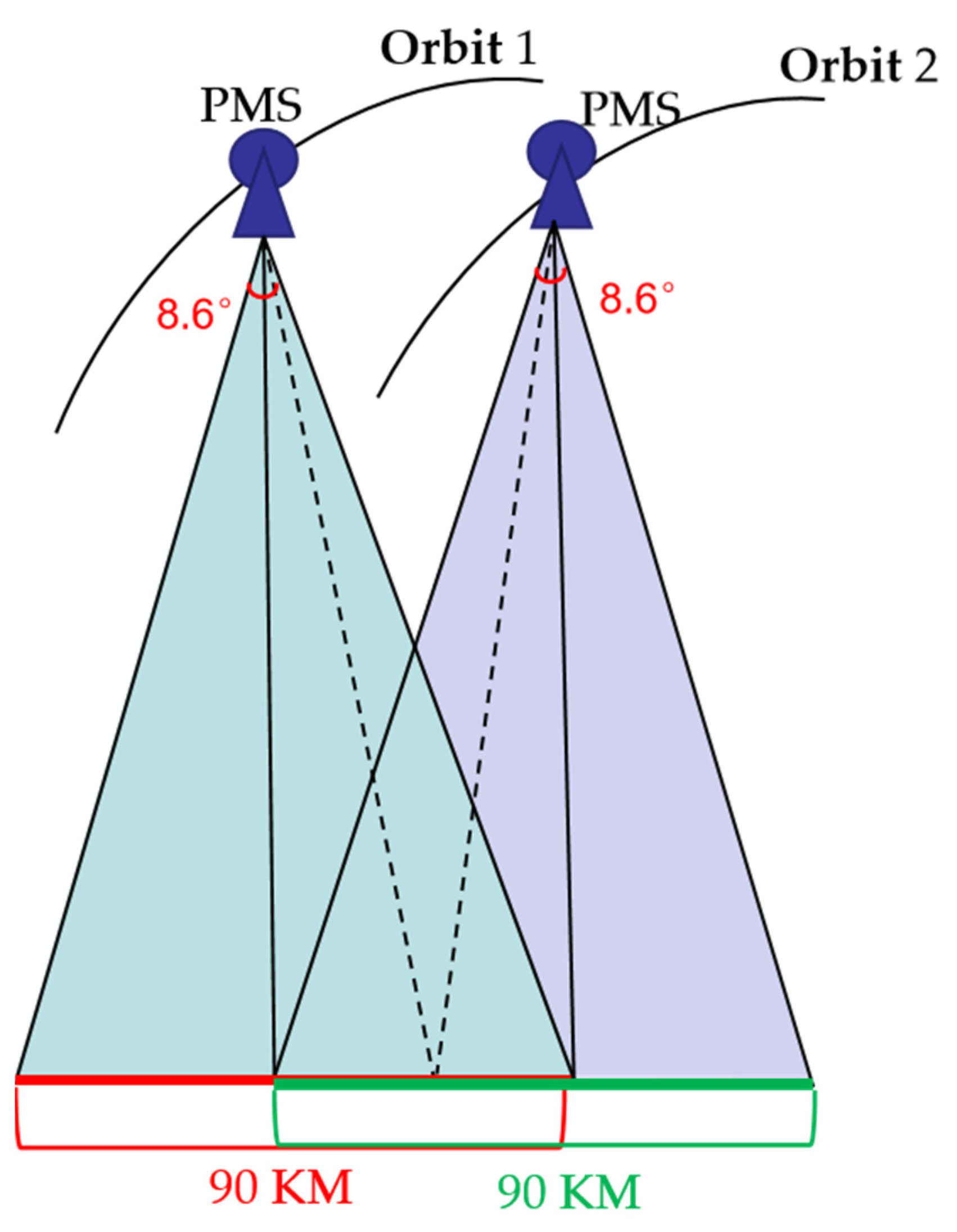
| Swath | ≈90 km | |
| Field of View | ≈8.6° | |
| Wide-Field-View (WFV) Camera | GSD | <16 m |
| Swath | ≈800 km | |
| Field of View | ≈64° | |
| Type | Object Accuracy/m | Image Accuracy/Pixel | ||||
|---|---|---|---|---|---|---|
| X | Y | Z | x | y | ||
| GCPs | Mean error | −0.0012 | 0.0002 | −0.0005 | 0.000 | 0.000 |
| RMSE | 0.4599 | 0.9717 | 6.3701 | 0.269 | 0.459 | |
| CKPs | Mean error | −0.0697 | −0.0613 | 0.9704 | 0.051 | −0.088 |
| RMSE | 0.5518 | 0.9013 | 5.5514 | 0.301 | 0.442 | |
| Region Type | Experimental Region | Elevation Accuracy of DSM Extracted by ENVI/DSM by This Paper/m | ||
|---|---|---|---|---|
| Mean Error | Absolute Mean Error | RMSE | ||
| Valley | Region 1 | 0.8116/0.148 | 29.990/7.981 | 42.917/11.087 |
| Region 2 | 0.093/0.510 | 19.285/6.333 | 33.673/8.700 | |
| Region 3 | 0.273/0.462 | 24.777/4.588 | 34.575/6.303 | |
| Ridge | Region 1 | 0.523/0.746 | 77.450/9.779 | 63.692/12.879 |
| Region 2 | 0.533/0.113 | 65.763/11.087 | 79.323/14.150 | |
| Region 3 | 0.445/0.674 | 65.445/10.321 | 78.305/13.606 | |
| Mountain peak | Region 1 | 0.974/0.051 | 113.73/14.599 | 141.30/20.301 |
| Region 2 | −8.611/0.389 | 103.27/14.101 | 128.16/19.043 | |
| Region 3 | 0.130/1.269 | 212.52/16.948 | 244.14/23.855 | |
| Urban | Region 1 | 0.326/0.105 | 31.125/10.594 | 42.281/14.929 |
Disclaimer/Publisher’s Note: The statements, opinions and data contained in all publications are solely those of the individual author(s) and contributor(s) and not of MDPI and/or the editor(s). MDPI and/or the editor(s) disclaim responsibility for any injury to people or property resulting from any ideas, methods, instructions or products referred to in the content. |
© 2023 by the authors. Licensee MDPI, Basel, Switzerland. This article is an open access article distributed under the terms and conditions of the Creative Commons Attribution (CC BY) license (https://creativecommons.org/licenses/by/4.0/).
Share and Cite
Yin, S.; Zhu, Y.; Hong, H.; Yang, T.; Chen, Y.; Tian, Y. DSM Extraction Based on Gaofen-6 Satellite High-Resolution Cross-Track Images with Wide Field of View. Sensors 2023, 23, 3497. https://doi.org/10.3390/s23073497
Yin S, Zhu Y, Hong H, Yang T, Chen Y, Tian Y. DSM Extraction Based on Gaofen-6 Satellite High-Resolution Cross-Track Images with Wide Field of View. Sensors. 2023; 23(7):3497. https://doi.org/10.3390/s23073497
Chicago/Turabian StyleYin, Suqin, Ying Zhu, Hanyu Hong, Tingting Yang, Yi Chen, and Yi Tian. 2023. "DSM Extraction Based on Gaofen-6 Satellite High-Resolution Cross-Track Images with Wide Field of View" Sensors 23, no. 7: 3497. https://doi.org/10.3390/s23073497