
Stochastic Modeling of Smartphones GNSS Observations Using LS-VCE and Application to Samsung S20


Abstract
:1. Introduction
2. Stochastic Modeling of Smartphone Observations Using Least-Square Variance Component Estimation
2.1. Least-Squares Variance Component Estimation (LS-VCE)
2.2. Application of LS-VCE Method to the Noise Assessment of the Smartphone Observations
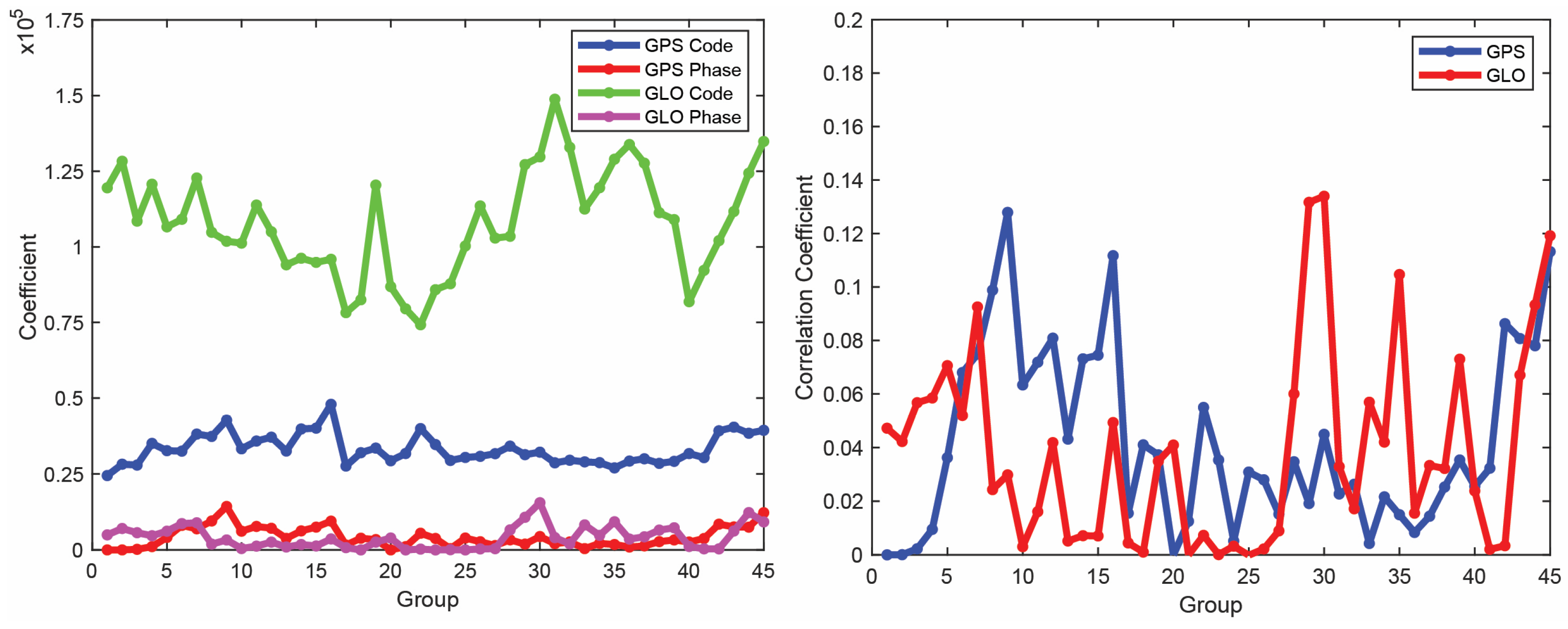
- For GPS: , indicating that code observables are 10 times noisier than the carrier phase observables, and indicating there is no correlation between the GPS code and phase observables;
- For GLONASS: indicating that GLONASS observables are times nosier than the GPS observables and indicating there is no correlation between the GLONASS code and carrier phase observables.
3. PPP Mathematical Model
3.1. Functional Model
3.2. Stochastic Model
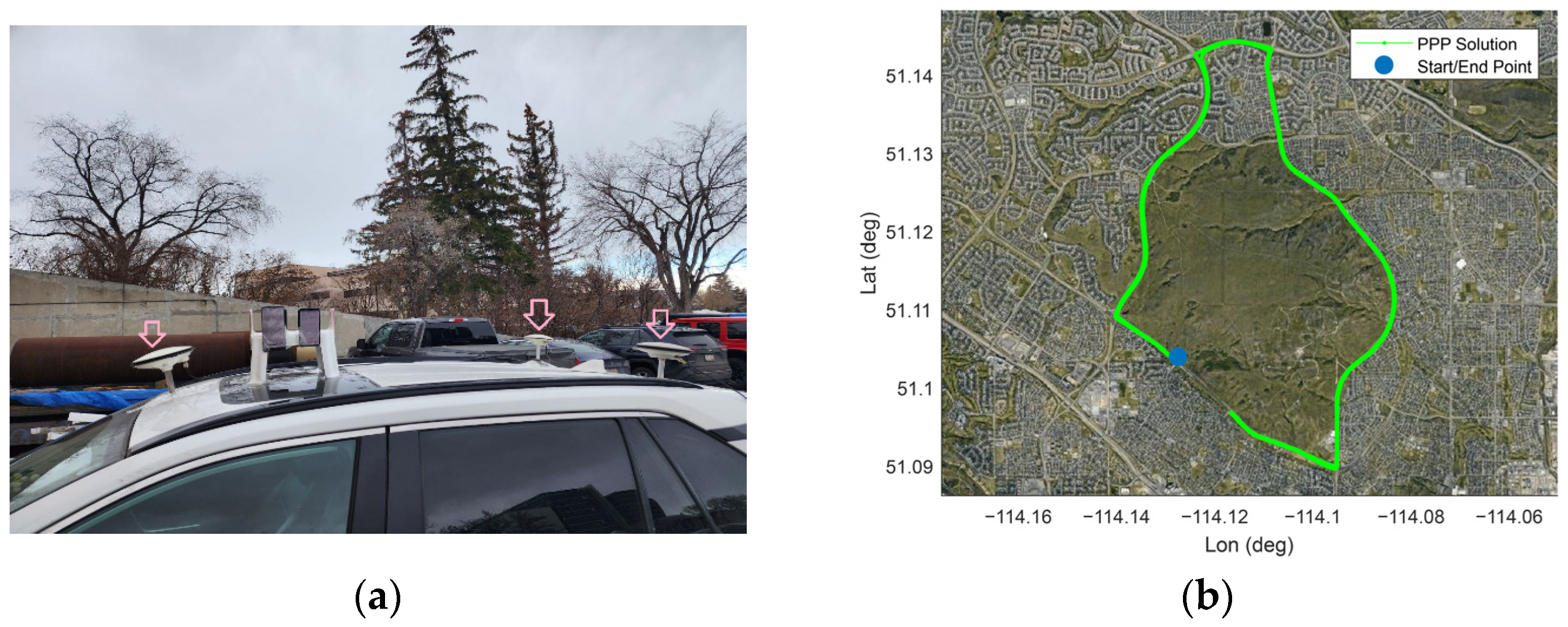
4. Experimental Results
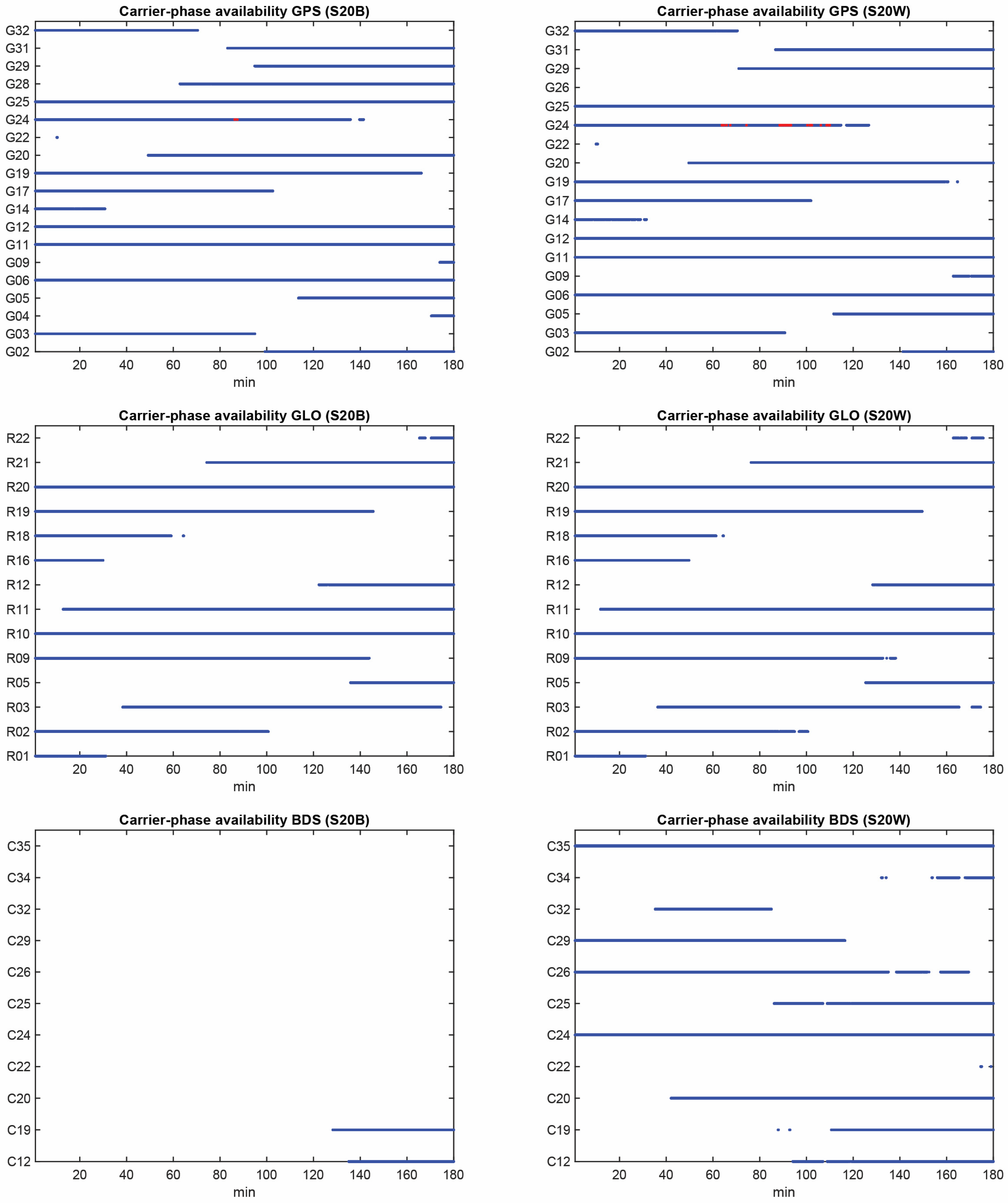
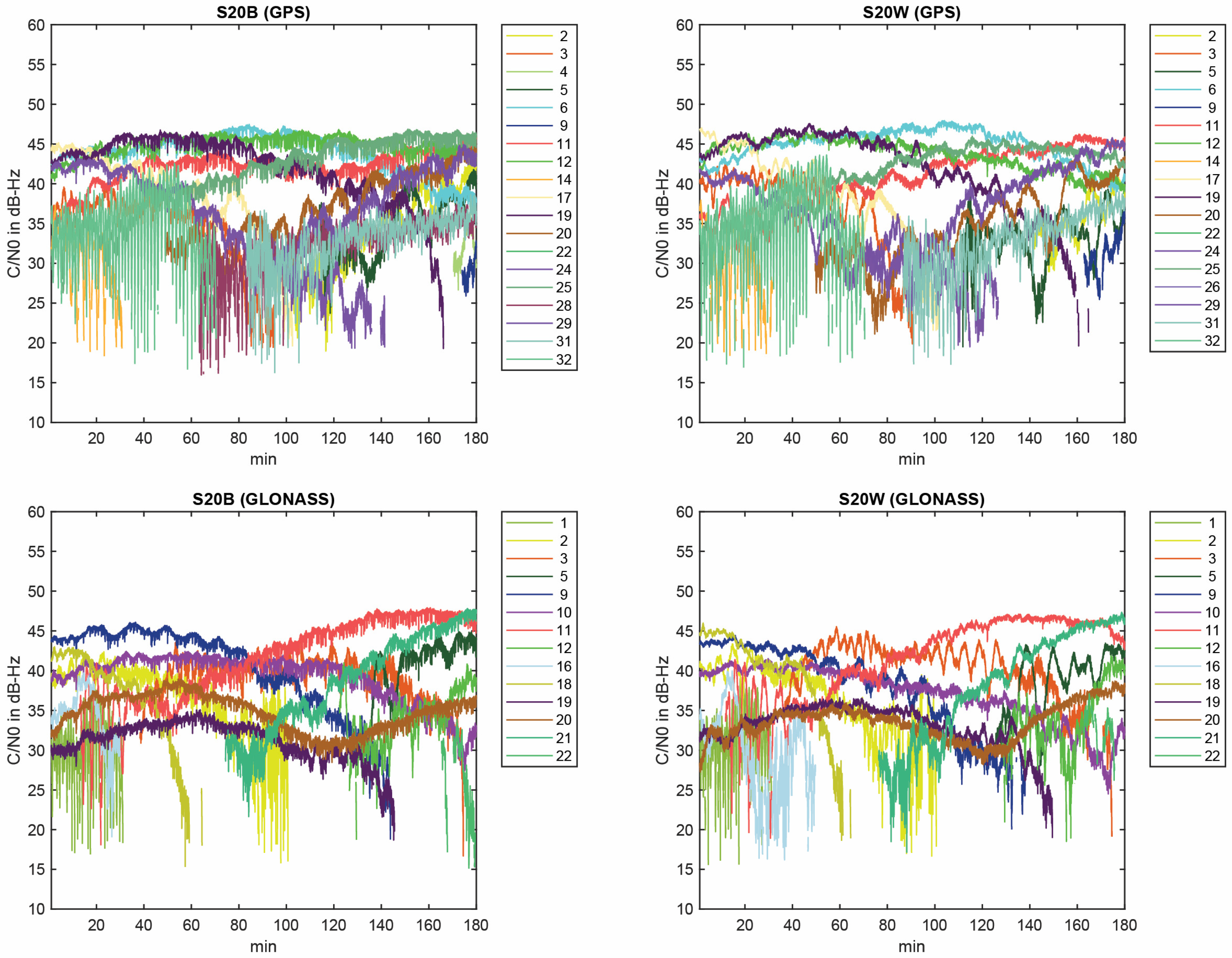
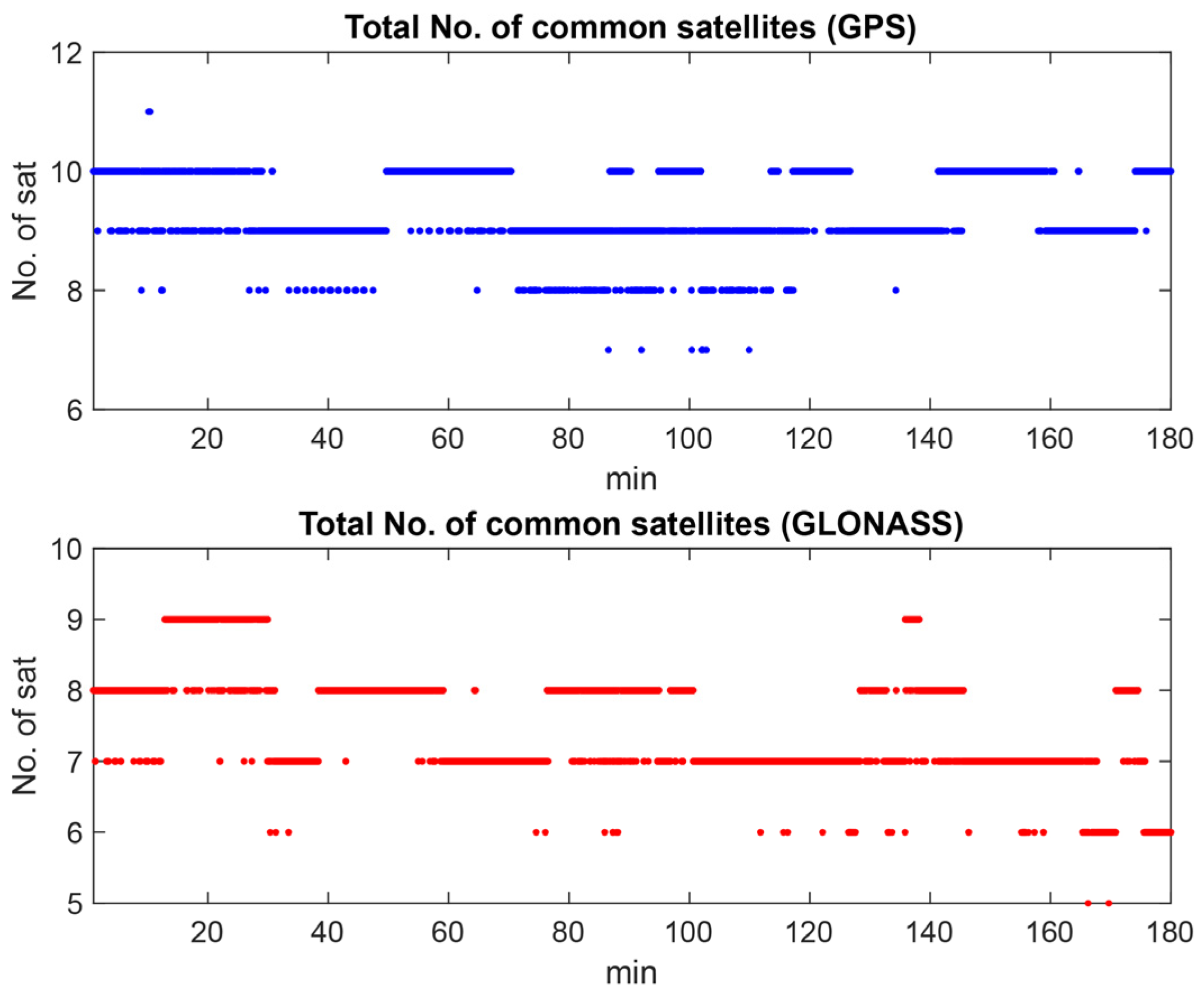
4.1. Noise Assessment of Samsung S20
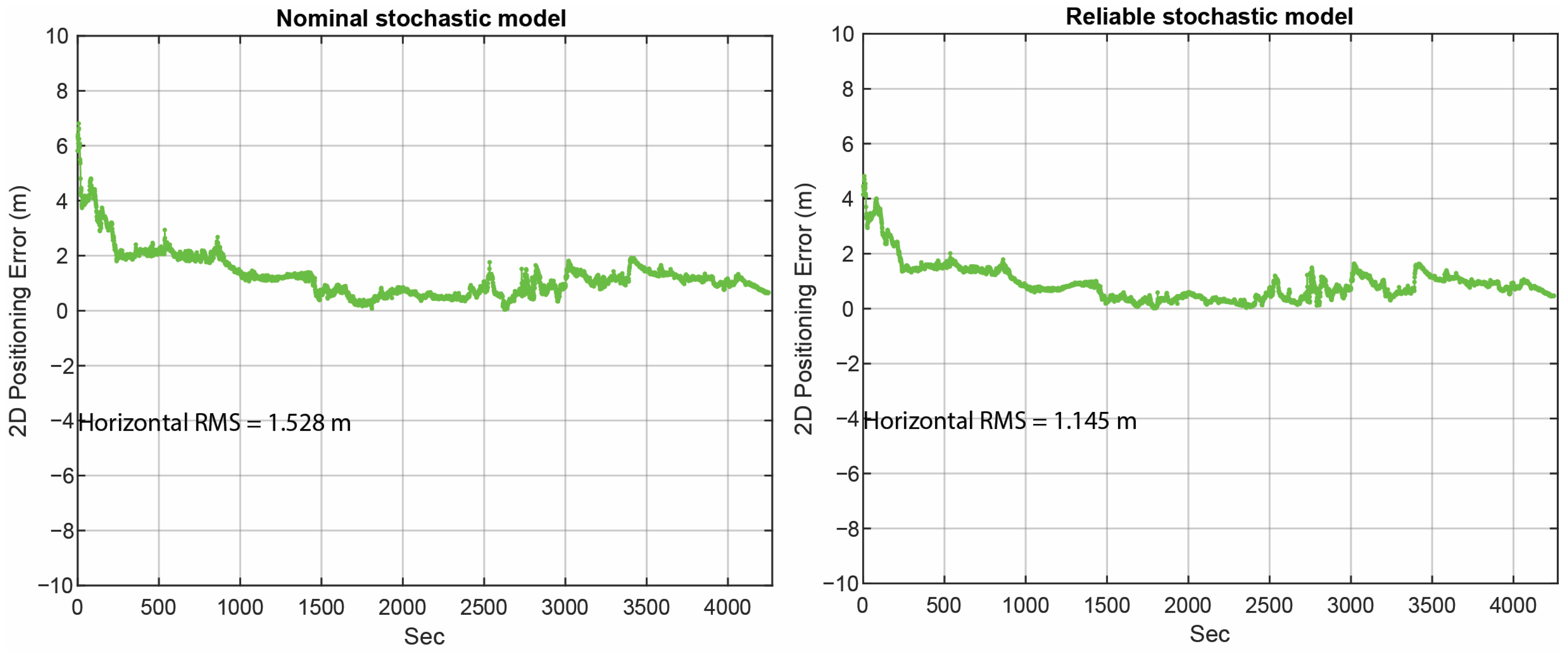
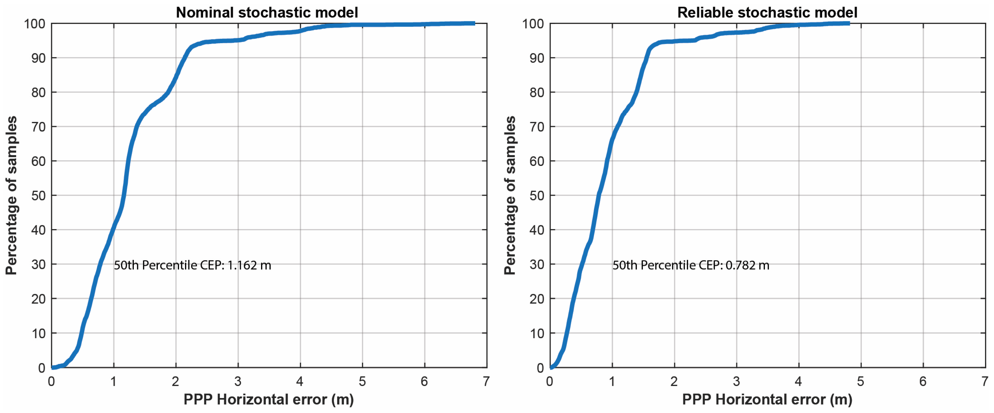
4.2. SF-PPP Performance Employing Reliable Stochastic Model
5. Summary and Conclusions
- The estimated coefficients for each constellation and each observation type are as follows: , for GPS and , for GLONASS as reported in Table 5;
- There is no significant correlation between the GPS code and carrier phase observations on the L1 frequency. The same conclusions hold for the GLONASS constellation;
- The results of the study confirmed an improvement of 25.1% and 32.7% on the RMS of horizontal positioning and the 50th percentile error, respectively, when employing the obtained stochastic model. This research provides insights into the potential of high-precision smartphone positioning and highlights the importance of the proper choice of functional and stochastic models in achieving this goal.
Author Contributions
Funding
Institutional Review Board Statement
Informed Consent Statement
Data Availability Statement
Acknowledgments
Conflicts of Interest
References
- Paziewski, J. Recent advances and perspectives for positioning and applications with smartphone GNSS observations. Meas. Sci. Technol. 2020, 31, 091001. [Google Scholar] [CrossRef]
- Zangenehnejad, F.; Gao, Y. GNSS smartphones positioning: Advances, challenges, opportunities, and future perspectives. Satell. Navig. 2021, 2, 24. [Google Scholar] [CrossRef] [PubMed]
- Shan, G.; Park, B.-H.; Nam, S.-H.; Kim, B.; Roh, B.-H.; Ko, Y.-B. A 3-dimensional triangulation scheme to improve the accuracy of indoor localization for IoT services. In Proceedings of the 2015 IEEE Pacific Rim Conference on Communications, Computers and Signal Processing (PACRIM), Victoria, BC, Canada, 24–26 August 2015; pp. 359–363. [Google Scholar] [CrossRef]
- Yoo, D.H.; Shan, G.; Roh, B.H. A vision-based indoor positioning systems utilizing computer aided design drawing. In Proceedings of the 28th Annual International Conference on Mobile Computing and Networking, Sydney, Australia, 17–21 October 2022; pp. 880–882. [Google Scholar]
- Shan, G.; Roh, B.-H. A slotted random request scheme for connectionless data transmission in bluetooth low energy 5.0. J. Netw. Comput. Appl. 2022, 207, 103493. [Google Scholar] [CrossRef]
- Zhu, N.; Marais, J.; Bétaille, D.; Berbineau, M. GNSS Position Integrity in Urban Environments: A Review of Literature. IEEE Trans. Intell. Transp. Syst. 2018, 19, 2762–2778. [Google Scholar] [CrossRef] [Green Version]
- Lee, W.; Patrick, G.; Yulin, Y.; Guoquan, H. Tightly-coupled GNSS-aided Visual-Inertial Localization. In Proceedings of the 2022 International Conference on Robotics and Automation (ICRA), Philadelphia, PA, USA, 23–27 May 2022; pp. 9484–9491. [Google Scholar]
- Asaad, S.M.; Halgurd, S.M. A comprehensive review of indoor/outdoor localization solutions in IoT era: Research challenges and future perspectives. Comput. Netw. 2022, 212, 109041. [Google Scholar] [CrossRef]
- Zumberge, J.F.; Heflin, M.B.; Jefferson, D.C.; Watkins, M.M.; Webb, F.H. Precise point positioning for the efficient and robust analysis of GPS data from large networks. J. Geophys. Res. Solid Earth 1997, 102, 5005–5017. [Google Scholar] [CrossRef] [Green Version]
- Kouba, J.; Héroux, P. Precise Point Positioning Using IGS Orbit and Clock Products. GPS Solutions 2001, 5, 12–28. [Google Scholar] [CrossRef]
- Langley, R. GPS receiver system noise. GPS World 1997, 8, 40–45. [Google Scholar]
- Liu, W.; Shi, X.; Zhu, F.; Tao, X.; Wang, F. Quality analysis of multi-GNSS raw observations and a velocity-aided positioning approach based on smartphones. Adv. Space Res. 2019, 63, 2358–2377. [Google Scholar] [CrossRef]
- Banville, S.; Lachapelle, G.; Ghoddousi-Fard, R.; Gratton, P. Automated processing of low-cost GNSS receiver data. In Proceedings of the 32nd International Technical Meeting of the Satellite Division of The Institute of Navigation (ION GNSS+ 2019), Miami, FL, USA, 16–20 September 2019; pp. 3636–3652. [Google Scholar]
- Shinghal, G.; Bisnath, S. Conditioning and PPP processing of smartphone GNSS measurements in realistic environments. Satell. Navig. 2021, 2, 10. [Google Scholar] [CrossRef]
- Paziewski, J.; Sieradzki, R.; Baryla, R. Signal characterization and assessment of code GNSS positioning with low-power consumption smartphones. GPS Solut. 2019, 23, 98. [Google Scholar] [CrossRef] [Green Version]
- Guo, L.; Wang, F.; Sang, J.; Lin, X.; Gong, X.; Zhang, W. Characteristics analysis of raw multi-GNSS measurement from Xiaomi Mi 8 and positioning performance improvement with L5/E5 frequency in an urban environment. Remote Sens. 2020, 12, 744. [Google Scholar] [CrossRef] [Green Version]
- Robustelli, U.; Paziewski, J.; Pugliano, G. Observation Quality Assessment and Performance of GNSS Standalone Positioning with Code Pseudoranges of Dual-Frequency Android Smartphones. Sensors 2021, 21, 2125. [Google Scholar] [CrossRef] [PubMed]
- Wang, L.; Li, Z.; Wang, N.; Wang, Z. Real-time GNSS precise point positioning for low-cost smart devices. GPS Solut. 2021, 25, 1–13. [Google Scholar] [CrossRef]
- Li, Y.; Cai, C.; Xu, Z. A Combined Elevation Angle and C/N0 Weighting Method for GNSS PPP on Xiaomi MI8 Smartphones. Sensors 2022, 22, 2804. [Google Scholar] [CrossRef] [PubMed]
- Miao, W.; Li, B.; Gao, Y. The superiority of multi-GNSS L5/E5a/B2a frequency signals in smartphones: Stochastic modelling, ambiguity resolution and RTK positioning. IEEE Internet Things J. 2022, 1. [Google Scholar] [CrossRef]
- Teunissen, P.J.G. Towards a Least-Squares Framework for Adjusting and Testing of Both Functional and Stochastic Model; Internal Research Memo, Geodetic Computing Centre: Delft, The Netherlands, 1988. [Google Scholar]
- Teunissen, P.J.G.; Amiri-Simkooei, A.R. Variance component estimation by the method of least-squares. In Proceedings of the 6th Hotine-Marussi Symp. of Theoretical and Computational Geodesy, IAG Symposia, Wuhan, China, 29 May–2 June 2006; Xu, P., Liu, J., Dermanis, A., Eds.; Springer: Berlin, Germany, 2006; Volume 132, pp. 273–279. [Google Scholar]
- Teunissen, P.J.G.; Amiri-Simkooei, A.R. Least-squares variance component estimation. J. Geodesy 2008, 82, 65–82. [Google Scholar] [CrossRef] [Green Version]
- Amiri-Simkooei, A.R. Least-Squares Variance Component Estimation: Theory and GPS Applications. Ph.D. Thesis, Delft University of Technology, Delft, The Netherlands, 2007. [Google Scholar]
- Amiri-Simkooei, A.R.; Teunissen, P.J.G.; Tiberius, C.C.J.M. Application of least-squares varinace component estimation to GPS observables. J. Surv. Eng. 2009, 135, 149–160. [Google Scholar] [CrossRef] [Green Version]
- Amiri-Simkooei, A.R.; Zangeneh-Nejad, F.; Asgari, J. Least-squares variance component estimation applied to GPS geometry-based observation model. J. Surv. Eng. 2013, 139, 176–187. [Google Scholar] [CrossRef]
- Amiri-Simkooei, A.R.; Jazaeri, S.; Zangeneh-Nejad, F.; Asgari, J. Role of stochastic model on GPS integer ambiguity resolution success rate. GPS Solut. 2015, 20, 51–61. [Google Scholar] [CrossRef]
- Zangenehnejad, F.; Gao, Y. Application of UofC model based multi-GNSS PPP to smartphones GNSS positioning. In Proceedings of the 34th International Technical Meeting of the Satellite Division of The Institute of Navigation (ION GNSS+ 2021), St. Louis, MO, USA, 20–24 September 2021; pp. 2986–3003. [Google Scholar]
- Teunissen, P.J.G.; Kleusberg, A. GPS for Geodesy, 2nd ed.; Springer-Verlag: Berlin/Heidelberg, Germany; New York, NY, USA, 1998. [Google Scholar]
- Héroux, P.; Gao, Y.; Kouba, J.; Lahaye, F.; Mireault, Y.; Collins, P.; Macleod, K.; Tetreault, P.; Chen, K. Products and applications for precise point positioning-moving towards real-time. In Proceedings of the 17th International Technical Meeting of the Satellite Division of The Institute of Navigation (ION GNSS 2004), Long Beach, CA, USA, 21–24 September 2004. [Google Scholar]
- Schaer, S.; Gurtner, W.; Feltens, J. IONEX: The ionosphere map exchange format version 1. In Proceedings of the IGS AC Work-shop, Darmstadt, Germany, 9–11 February 1998; Volume 9. [Google Scholar]
- Dach, R.; Lutz, S.; Walser, P.; Fridez, P. Bernese GNSS Software, Version 5.2; Astronomical Institute, University of Bern: Bern, Switzerland, 2015. [Google Scholar]
- Zangenehnejad, F.; Jiang, Y.; Gao, Y. GNSS Observation Generation from Smartphone Android Location API: Performance of Existing Apps, Issues and Improvement. Sensors 2023, 23, 777. [Google Scholar] [CrossRef]
- Yong, C.Z.; Odolinski, R.; Zaminpardaz, S.; Moore, M.; Rubinov, E.; Er, J.; Denham, M. Instantaneous, dual-frequency, multi-GNSS precise RTK positioning using google pixel 4 and Samsung Galaxy S20 smartphones for zero and short baselines. Sensors 2021, 21, 8318. [Google Scholar] [CrossRef] [PubMed]
- Liu, F.; Elsheikh, M.; Gao, Y.; El-Sheimy, N. Fast convergence real-time precise point positioning with Android smartphone GNSS data. In Proceedings of the 34th International Technical Meeting of the Satellite Division of The Institute of Navigation (ION GNSS+ 2021), St. Louis, MO, USA, 20–24 September 2021; pp. 3049–3058. [Google Scholar]
- Wu, Q.; Sun, M.; Zhou, C.; Zhang, P. Precise Point Positioning Using Dual-Frequency GNSS Observations on Smartphone. Sensors 2019, 19, 2189. [Google Scholar] [CrossRef] [PubMed] [Green Version]
- Chen, B.; Gao, C.; Liu, Y.; Sun, P. Real-time Precise Point Positioning with a Xiaomi MI 8 Android Smartphone. Sensors 2019, 19, 2835. [Google Scholar] [CrossRef] [Green Version]
- Zhu, H.; Xia, L.; Wu, D.; Xia, J.; Li, Q. Study on Multi-GNSS precise point positioning performance with adverse effects of satellite signals on Android smartphone. Sensors 2020, 20, 6447. [Google Scholar] [CrossRef] [PubMed]


| Pillar | N2 |
|---|---|
| Y (m) | −1,641,898.085 |
| Y (m) | −3,664,875.558 |
| Z (m) | 4,939,969.351 |
| Lat. (Deg.) | 51.07942671 |
| Lon. (Deg.) | −114.13282014 |
| H (m) | 1116.589 |
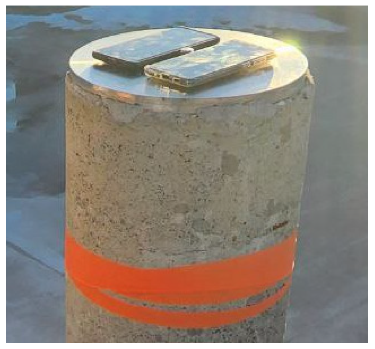
| Device | Samsung S20 Black (S20B) and Samsung S20 White (S20W) |
| Constellations | GPS (Yes), GLONASS (Yes), Galileo (No observation recorded), BeiDou (Yes), and QZSS (Yes) |
| Mode | Static |
| App logger | GnssLogger (v3.0.5.6) |
| RINEX converter | UofC CSV2RINEX tool [33] |
| Date | 4 February 2023 |
| Duration | 3 h |
| Sampling interval | 1 s |
| Observation Type | Parameter | GPS | GLONASS |
|---|---|---|---|
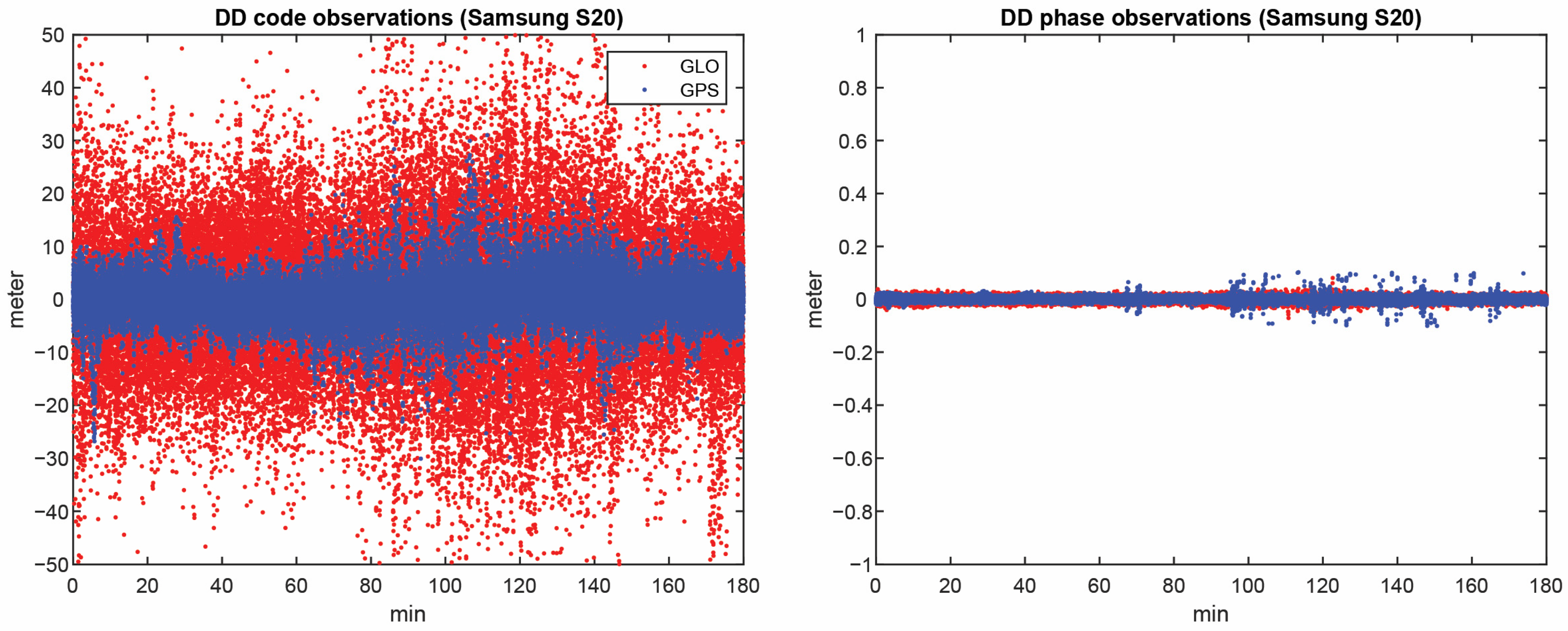
| Code | Mean | 0.126 | 0.001 |
| RMS | 3.408 | 13.596 | |
| Phase | Mean | 0.001 | 0.001 |
| RMS | 0.01 | 0.009 |
| Constellation | |||
|---|---|---|---|
| GPS | 0.35 × 10⁵ | 0.04 × 10⁵ | 0.04 |
| GLONASS | 1.08 × 10⁵ | 0.04 × 10⁵ | 0.03 |
| Device | Samsung S20 Black |
| App logger | GnssLogger (v3.0.5.6) |
| RINEX converter | UofC CSV2RINEX tool [32] |
| Measurements used | GPS (L1), GLONASS (L1) |
| Mode | Kinematic |
| Date | 22 November 2022 |
| Duration | 1 h |
| Sampling interval | 1 s |
| Troposphere model | Saastamoinen model |
| Ionosphere model | Global ionospheric maps (GIM) |
| Functional model | SF PPP model |
| Stochastic model | C/N0 and elevation weighting function (nominal and estimated stochastic model) |
| Elevation mask angle | 10 deg |
| C/N0 mask | 20 dB-Hz |
| Satellite orbit | CODE MGEX precise ephemerides (5 min interval) |
| Clock error | CODE MGEX precise clock (1 s interval) |
| Satellite DCB correction | CAS DCBs in Bias SINEX (BSX) format |
Disclaimer/Publisher’s Note: The statements, opinions and data contained in all publications are solely those of the individual author(s) and contributor(s) and not of MDPI and/or the editor(s). MDPI and/or the editor(s) disclaim responsibility for any injury to people or property resulting from any ideas, methods, instructions or products referred to in the content. |
© 2023 by the authors. Licensee MDPI, Basel, Switzerland. This article is an open access article distributed under the terms and conditions of the Creative Commons Attribution (CC BY) license (https://creativecommons.org/licenses/by/4.0/).
Share and Cite
Zangenehnejad, F.; Gao, Y. Stochastic Modeling of Smartphones GNSS Observations Using LS-VCE and Application to Samsung S20. Sensors 2023, 23, 3478. https://doi.org/10.3390/s23073478
Zangenehnejad F, Gao Y. Stochastic Modeling of Smartphones GNSS Observations Using LS-VCE and Application to Samsung S20. Sensors. 2023; 23(7):3478. https://doi.org/10.3390/s23073478
Chicago/Turabian StyleZangenehnejad, Farzaneh, and Yang Gao. 2023. "Stochastic Modeling of Smartphones GNSS Observations Using LS-VCE and Application to Samsung S20" Sensors 23, no. 7: 3478. https://doi.org/10.3390/s23073478