
A Two-Stage Multi-Agent EV Charging Coordination Scheme for Maximizing Grid Performance and Customer Satisfaction
 , , ,
, , ,
Abstract
:1. Introduction
2. Related Work
- A two-stage coordination framework for EV charging and scheduling is presented to maximize network performance and customer charging satisfaction;
- Various indices for power loss, voltage profile, charging cost and waiting time are devised for the coordinated charging operation of EVs, and the customers’ charging satisfaction is investigated with the time of use (ToU) and real-time pricing (RTP);
- The coordinated framework among muti EV aggregator agents is established to manage the charging activities at residential and workplace platforms;
- The proposed approach bears a low computational burden.
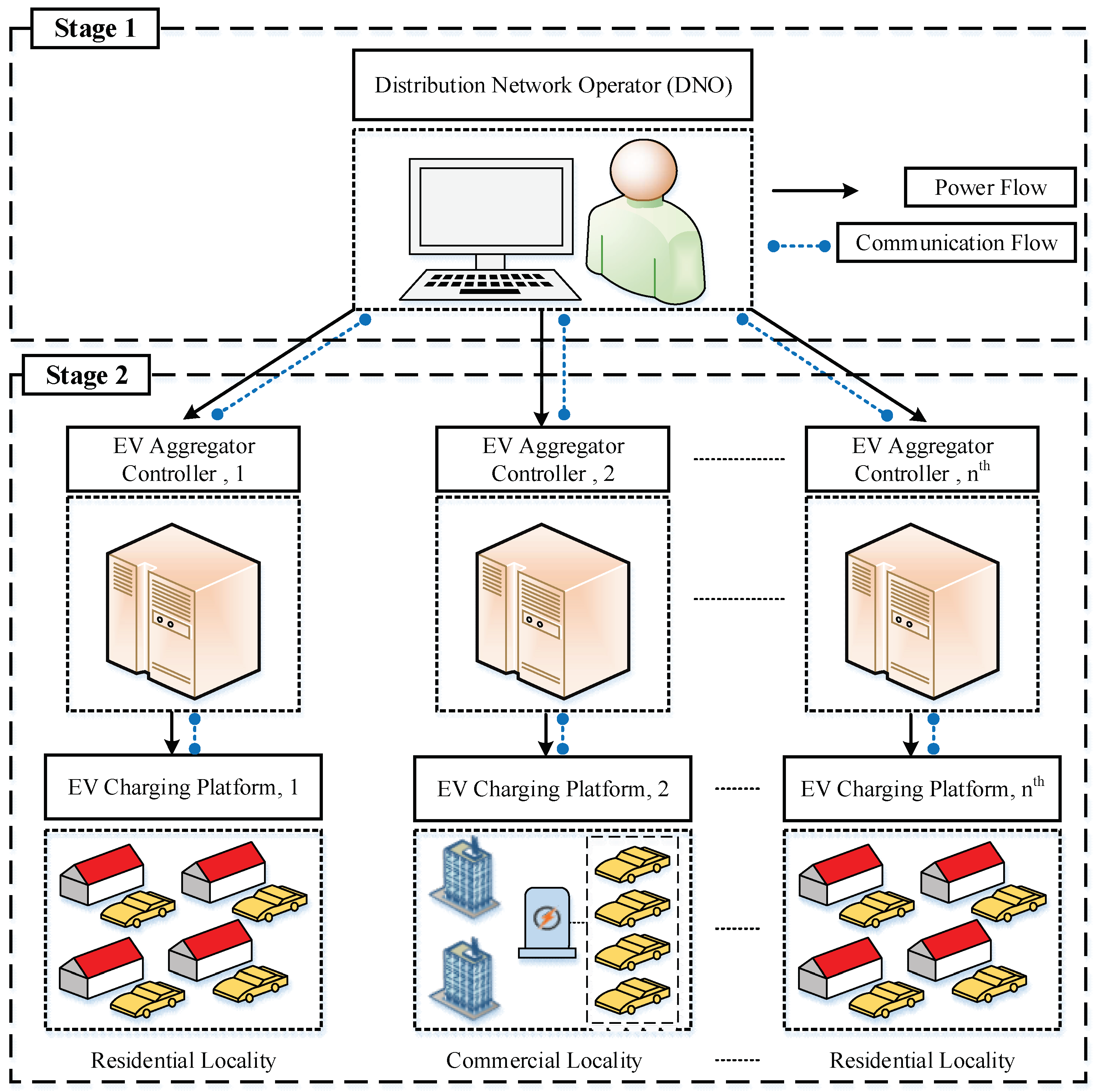
3. AECM Architecture
4. Two-Stage EV Charging Management Strategy
4.1. Scenario Design
4.2. Stage-1: Power Distribution to the Aggregators
Constraints
- Voltage Limits:
- Power Allocation and Distribution Constraints
- Instantaneous Maximum Demand Constraint
4.3. Stage-2: Coordinated EV Charging
Constraints
- Stay Time Constraint
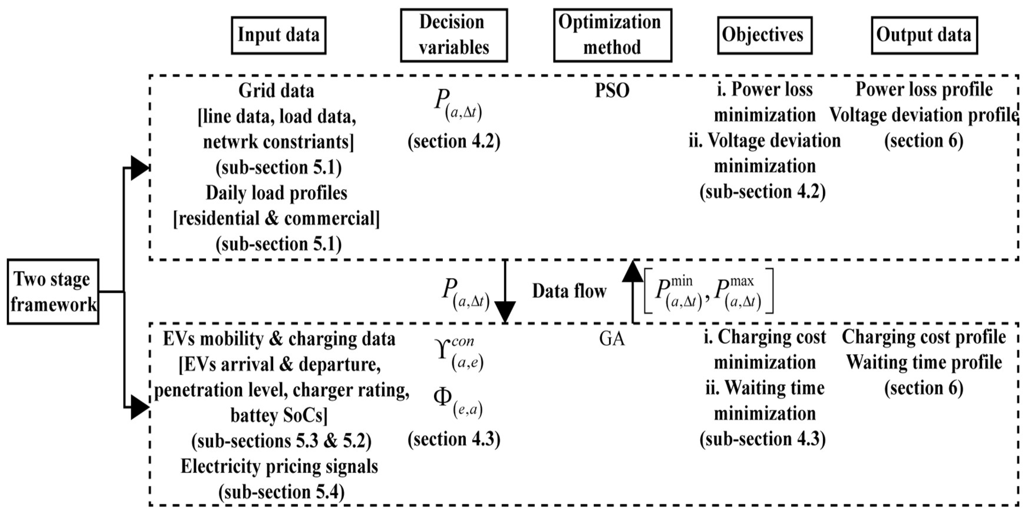
4.4. Proposed Research Design with Information Exchange and Control Process
4.4.1. Steps for Stage-1
- i.
- Input Data
- ii.
- Decision Variables
- iii.
- Objective Function
- iv.
- Optimization Method
- v.
- Output data
4.4.2. Steps for Stage-2
- i.
- Input Data
- ii.
- Decision Variables
- iii.
- Objective Function
- iv.
- Optimization Method
- v.
- Output Data
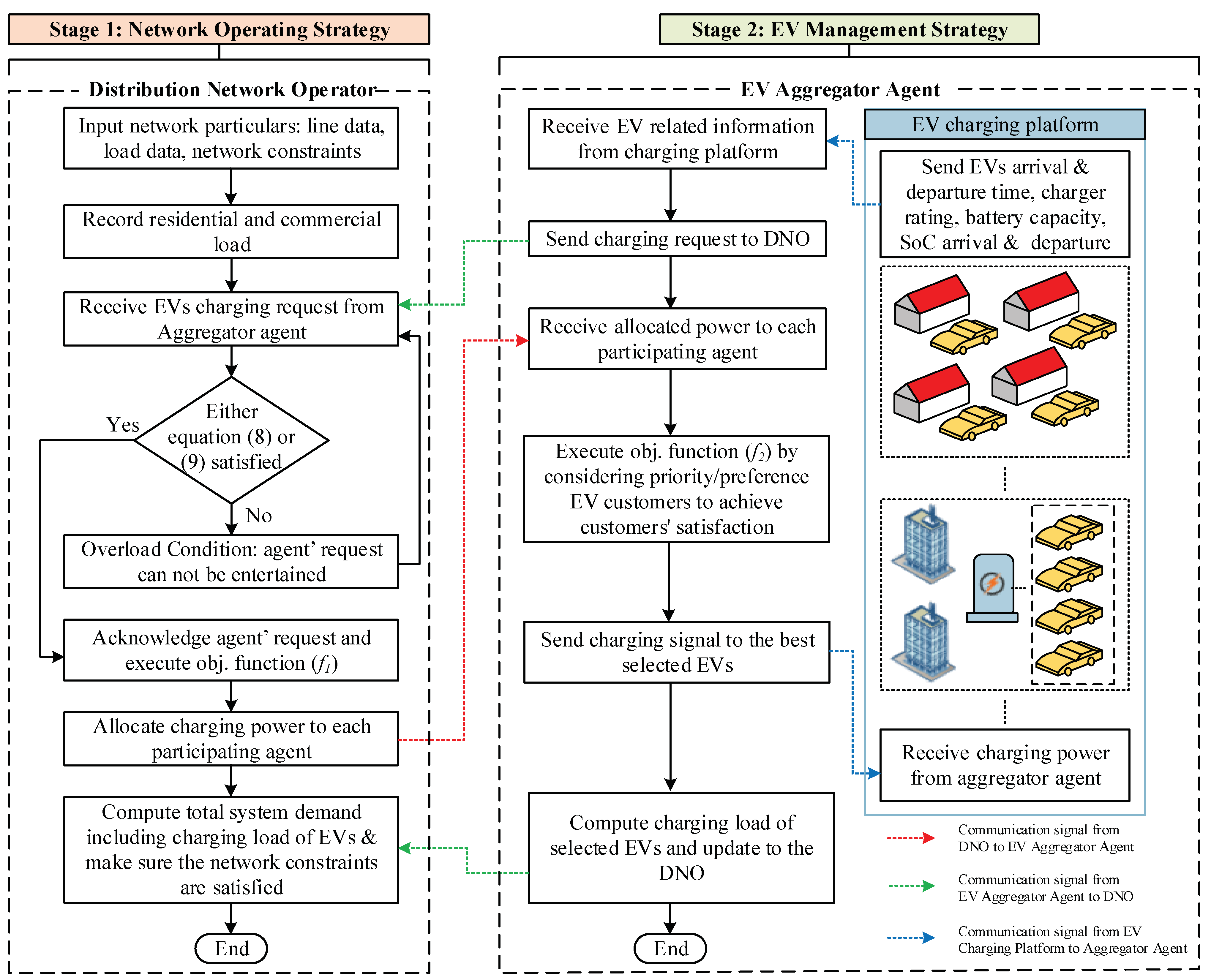
- Step 1:
- The DNO records the residential and commercial load profiles for each time interval .
- Step 2:
- The EV aggregator agent receives the charging information from the EVs operating in its territory. The information includes: arrival time , departure time , SoC at the arrival , requested SoC at departure and customer charging preference/priority. Each participating EV aggregator agent requests the DNO for the allocation of charging power.
- Step 3:
- The DNO checks the condition of the maximum demand limit for both residential and commercial feeders, i.e., and . Once the condition is met, the DNO executes the objective function (f1) and allocates the charging power to each participating agent.
- Step 4:
- The participating agents receive the allocated power to fulfil the charging demand of EVs.
- Step 5:
- The EV aggregator agents execute the objective function (f2) by considering customers’ preference/priorities.
- Step 6:
- The EV aggregator agents then send the charging signal to the best selected EVs to start charging.
- Step 7:
- Once the charging process starts, the EV aggregator agents compute the charging load and update the DNO about it.
- Step 8:
- After receiving the information about the connected load of EVs, the DNO makes sure that the connected charging load does not have any effect on the network performance.
| Algorithm 1. Power Allocation to EV Aggregator Agents |
| Input:, |
| Output: |
|
| End process |
| Algorithm 2: Power Allocation to EV Aggregator Agents |
| Input:, ToU, RTP price signal. |
| Output: considering their preferences. |
|
| end while |
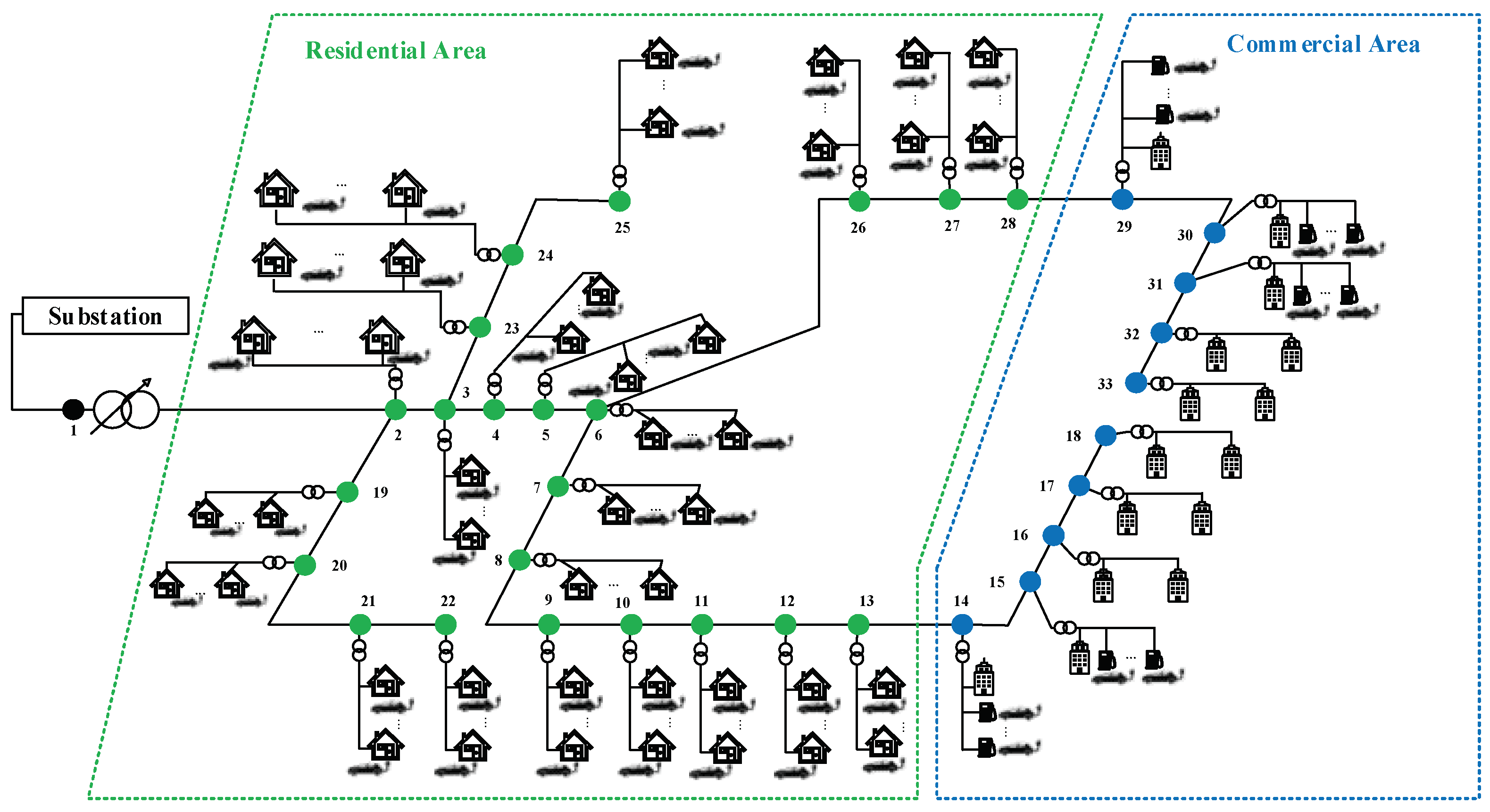
5. Test System and Simulation Setup
5.1. Test System
5.2. EV Fleet Specifications
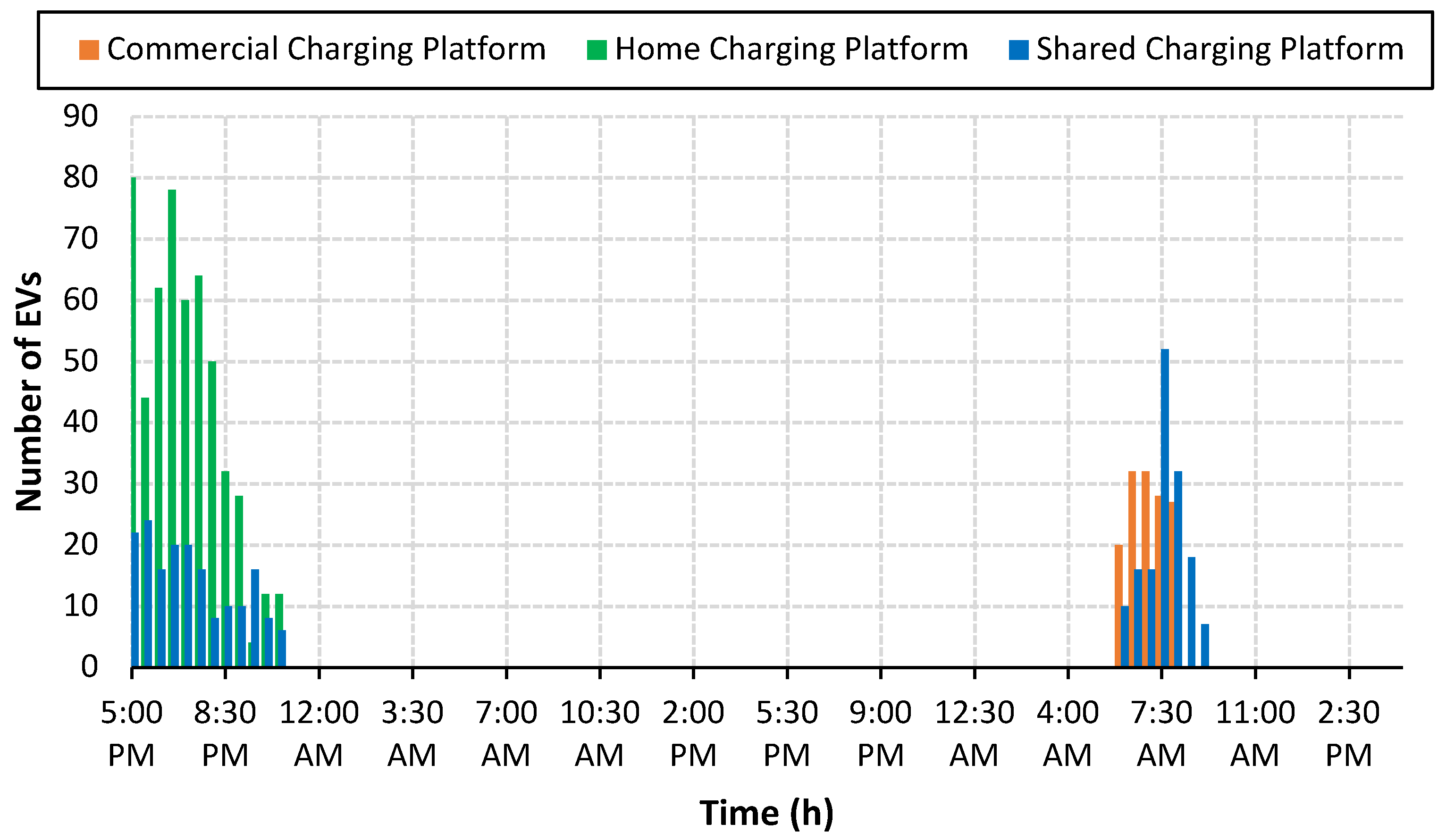
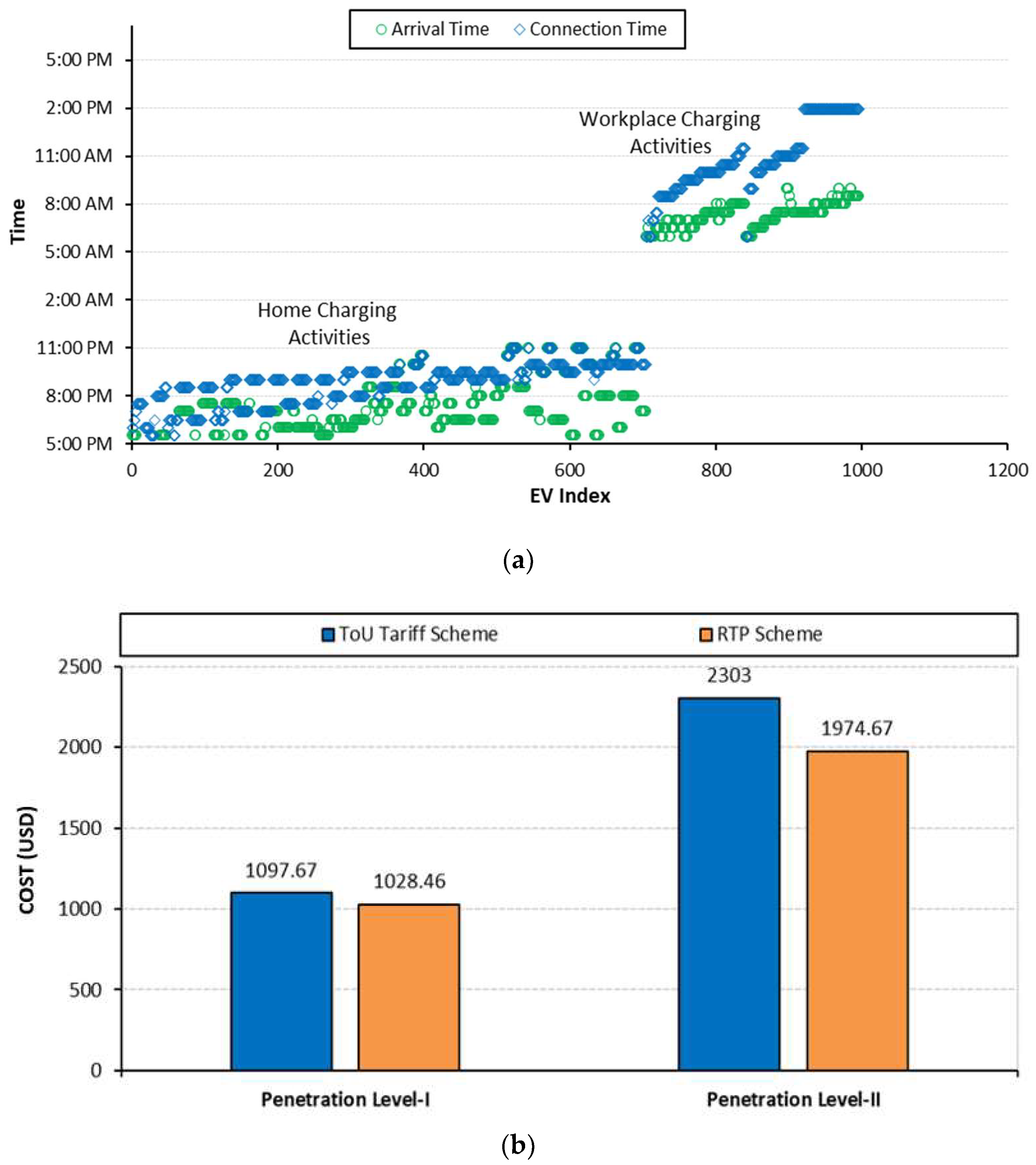
5.3. EVs Mobility Behaviour
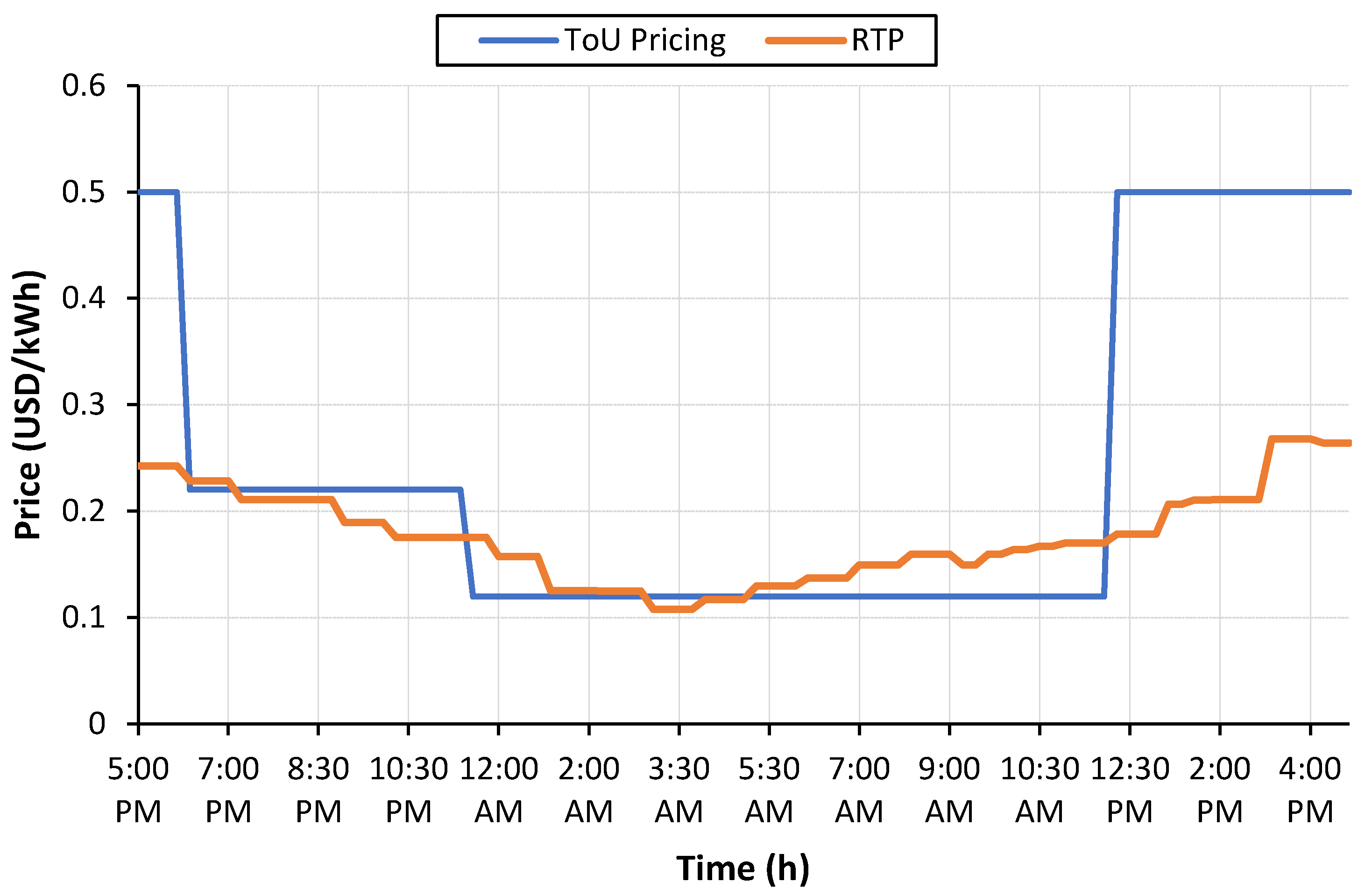
5.4. Electricity Pricing Schemes
6. Results and Discussion
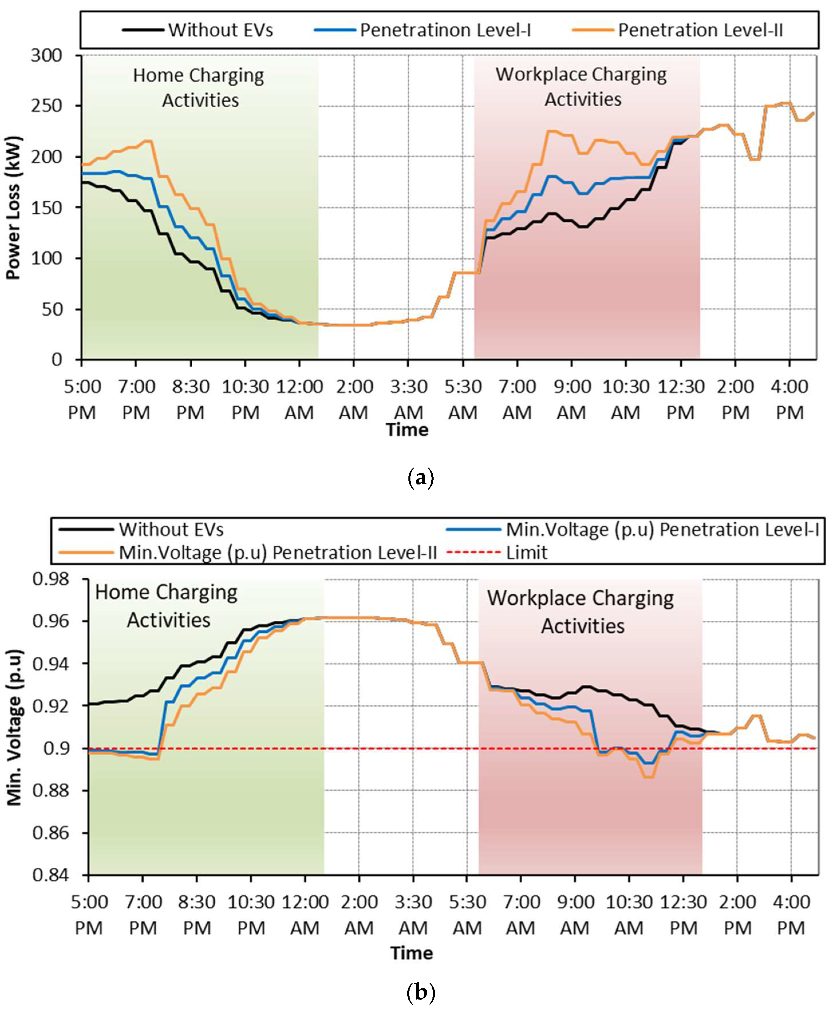
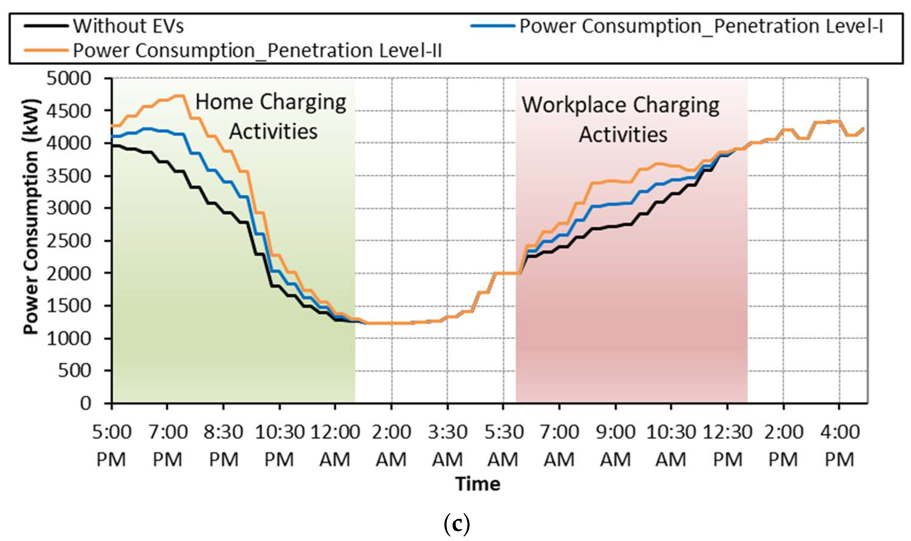
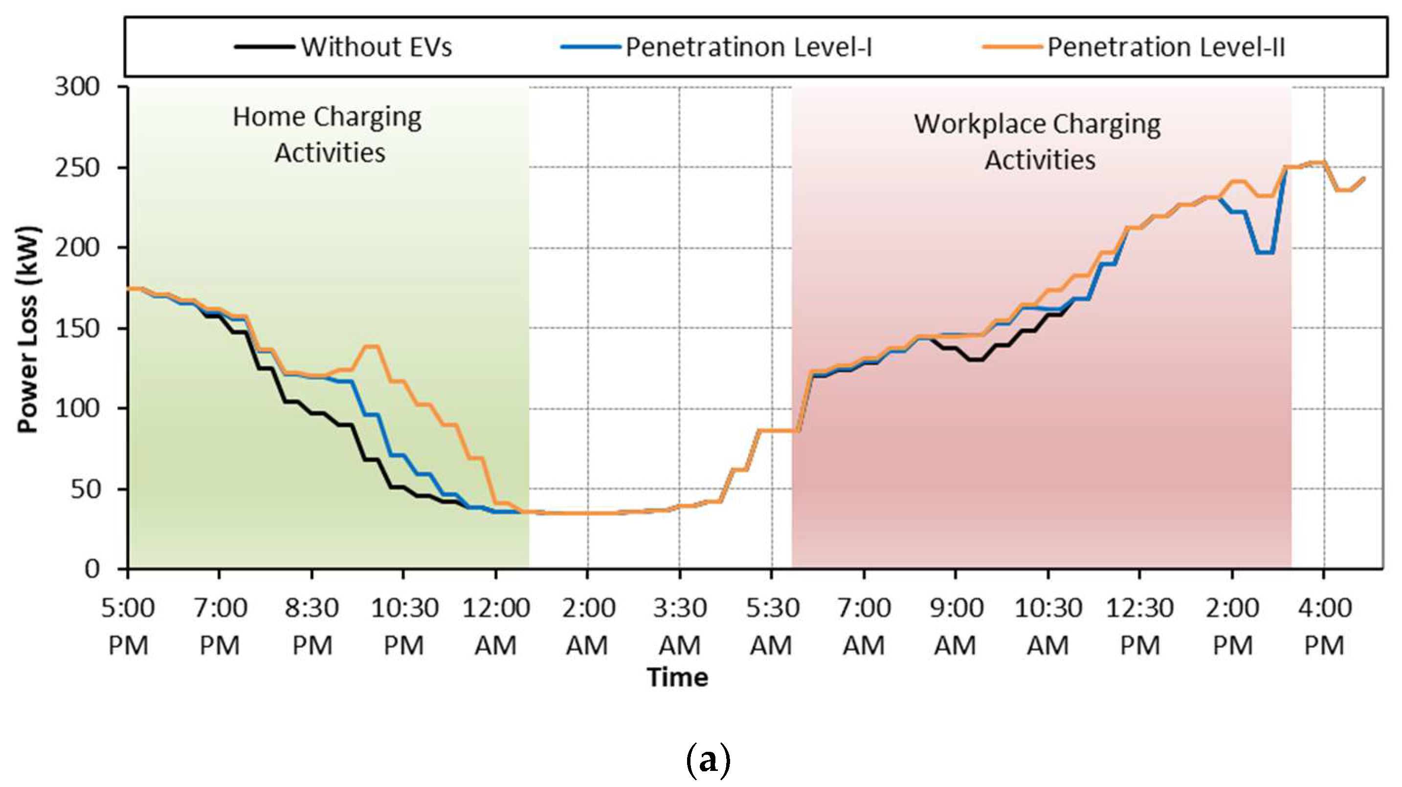
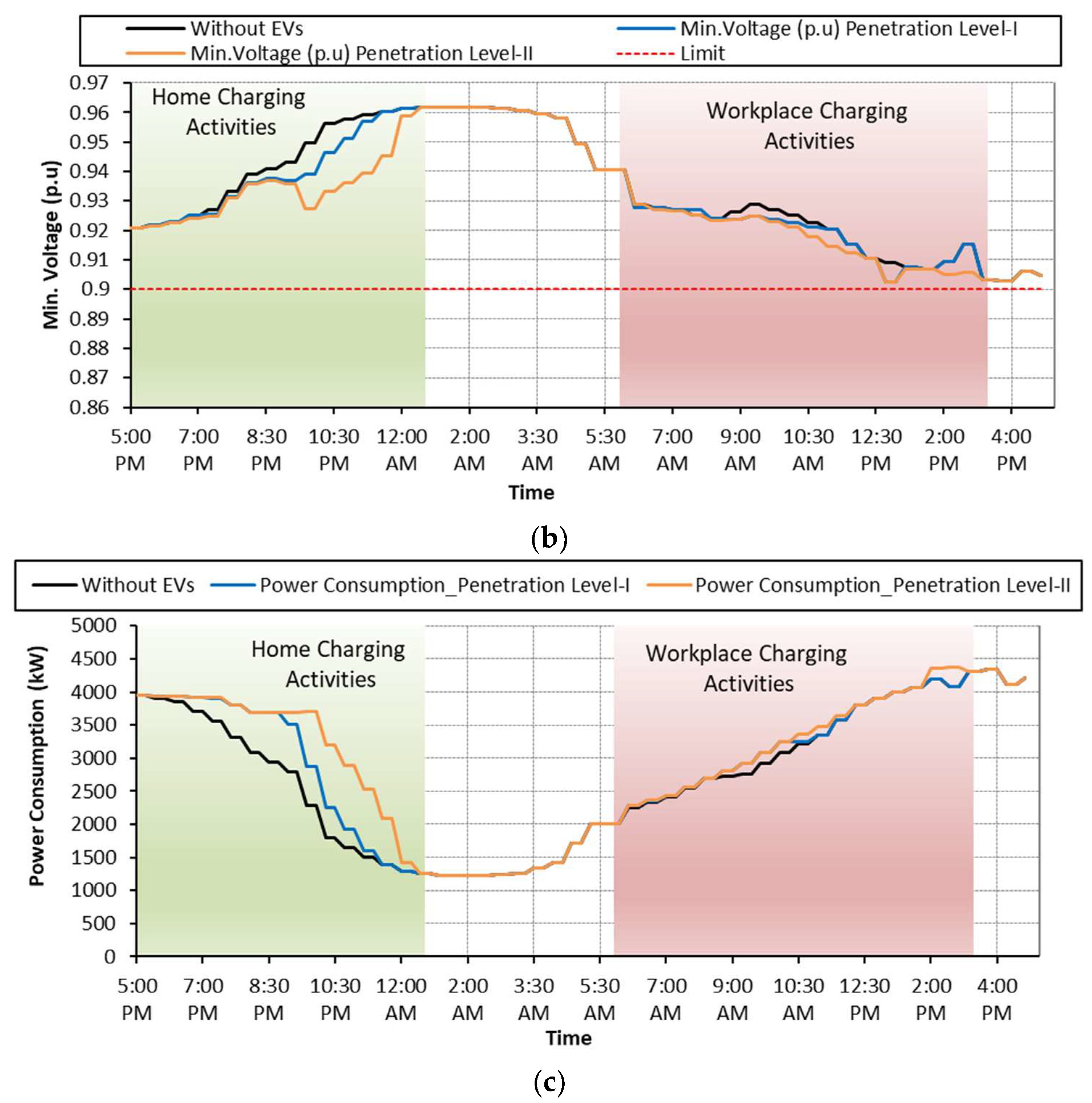
6.1. Case: A: Uncoordinated EV Charging
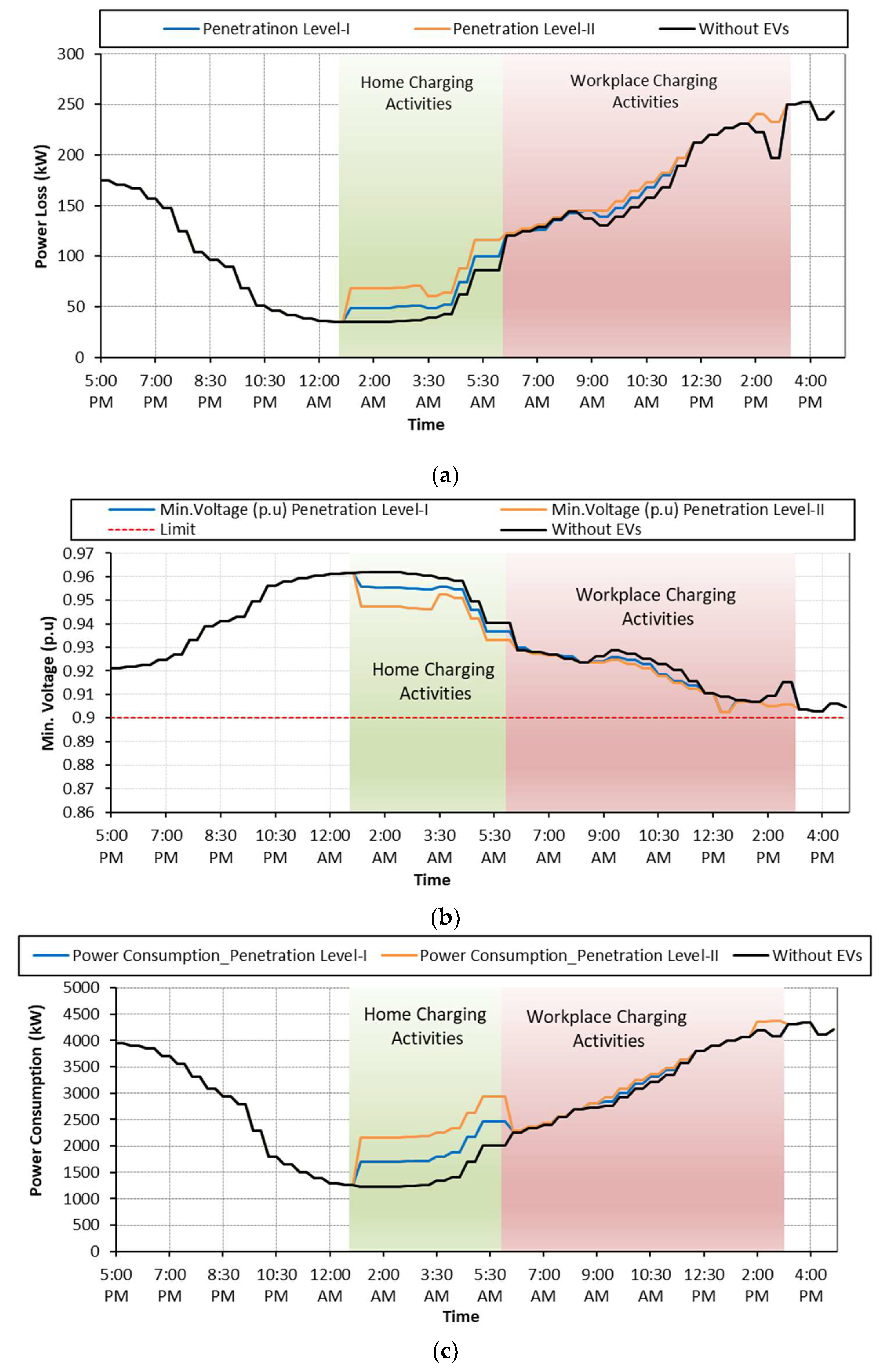
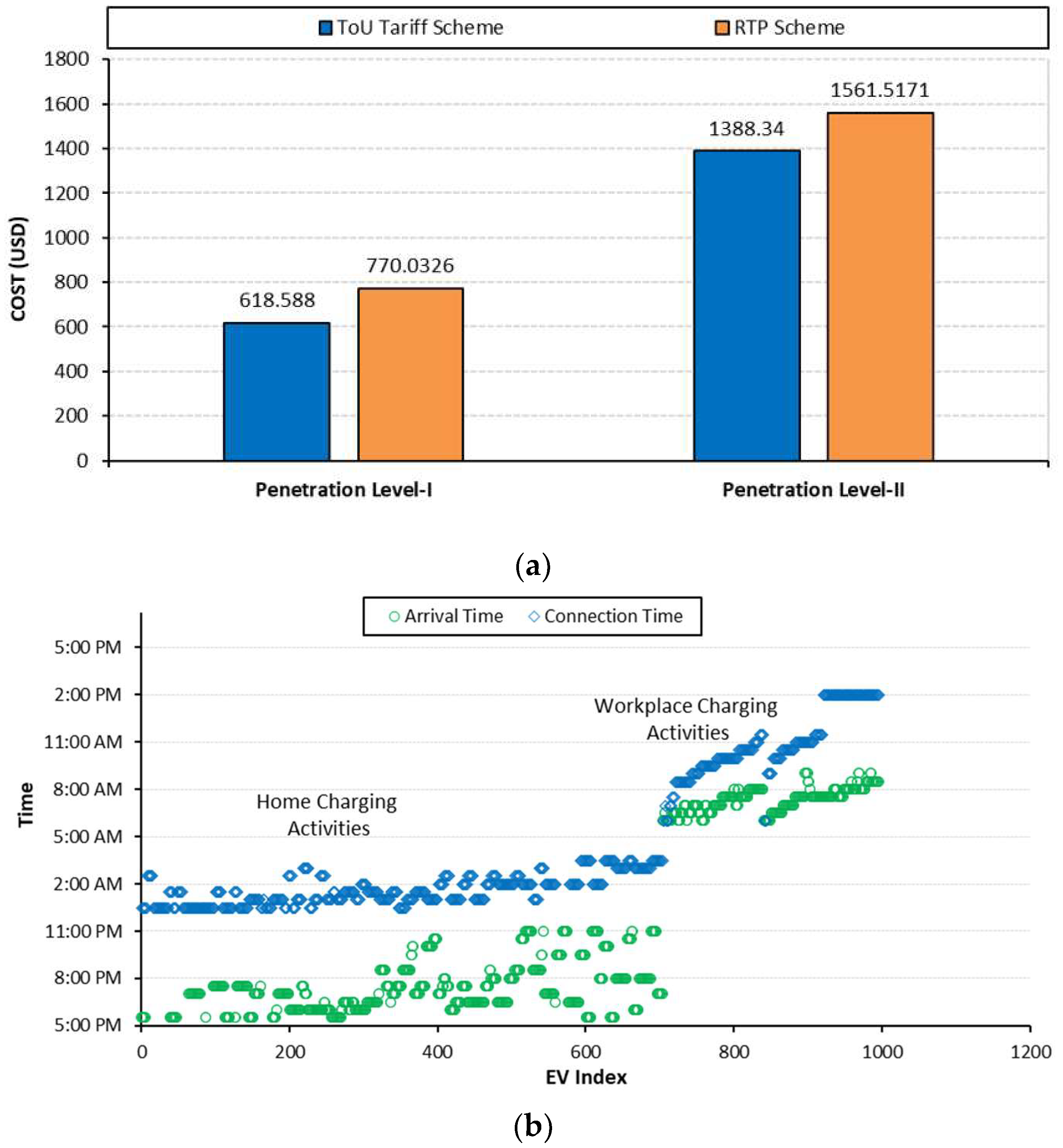
6.2. Case: B: Coordinated EV Charging with ToU and RTP Tariff for Waiting Time Minimization
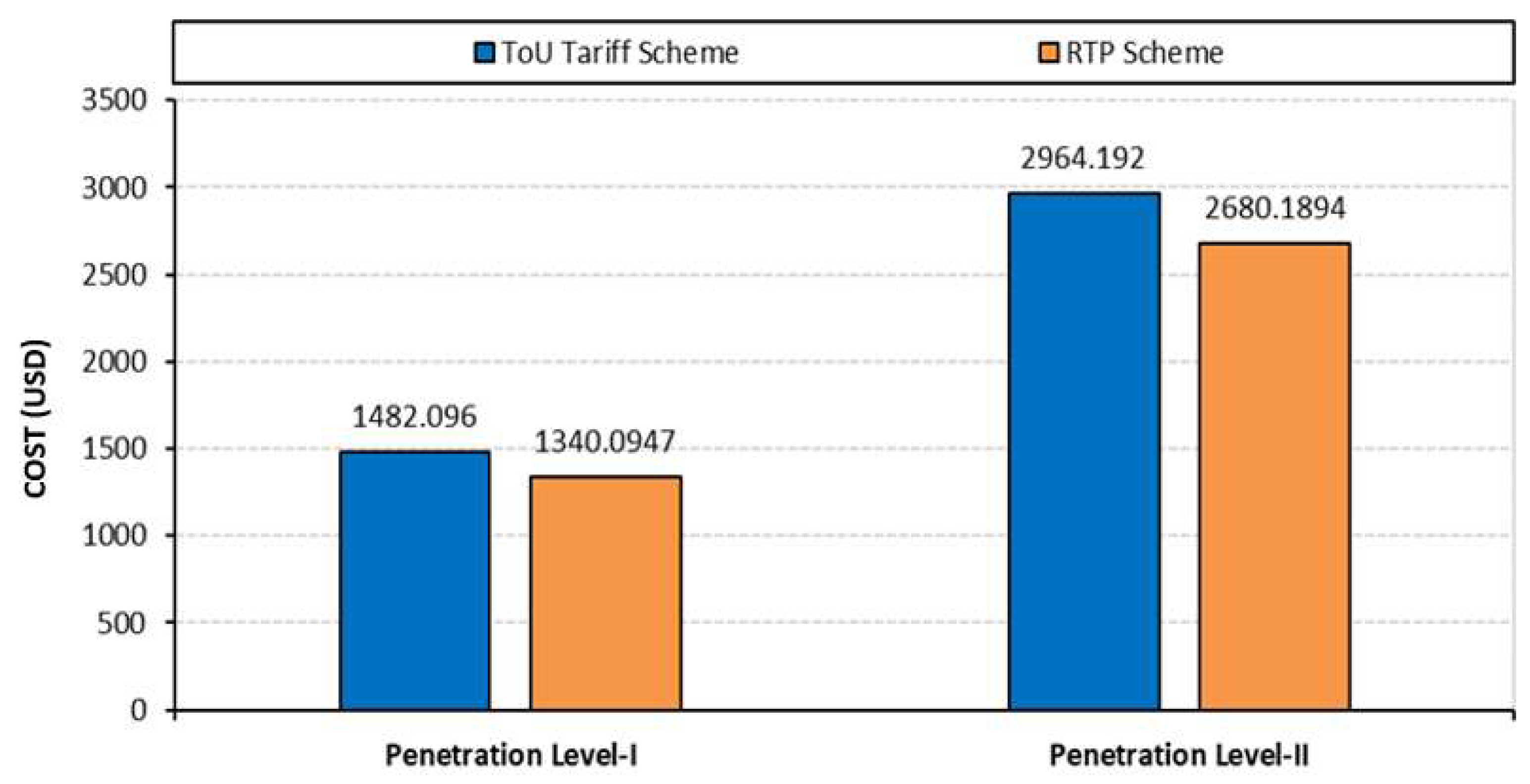
6.3. Case: C: Coordinated EV Charging with ToU tariff and RTP for Charging Cost Minimization
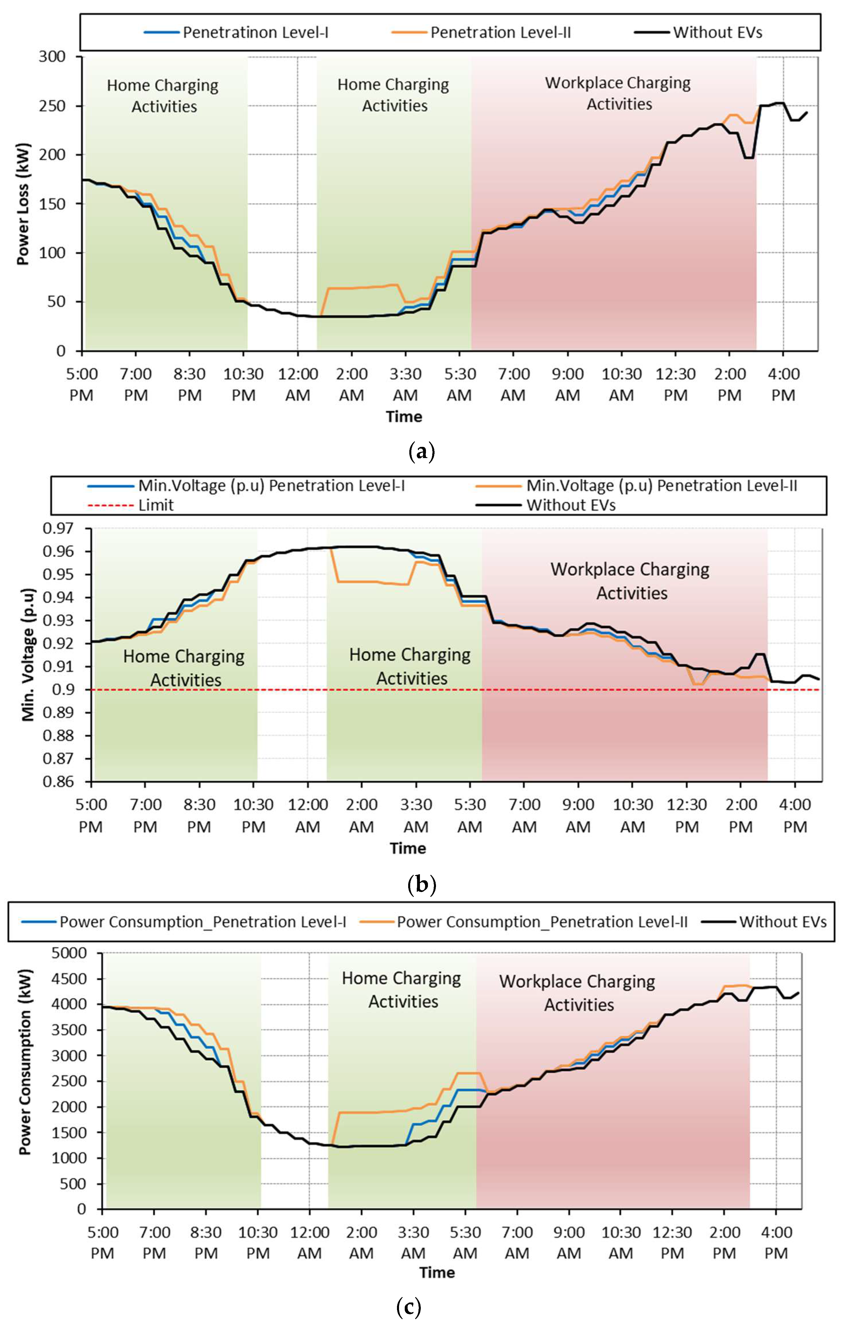
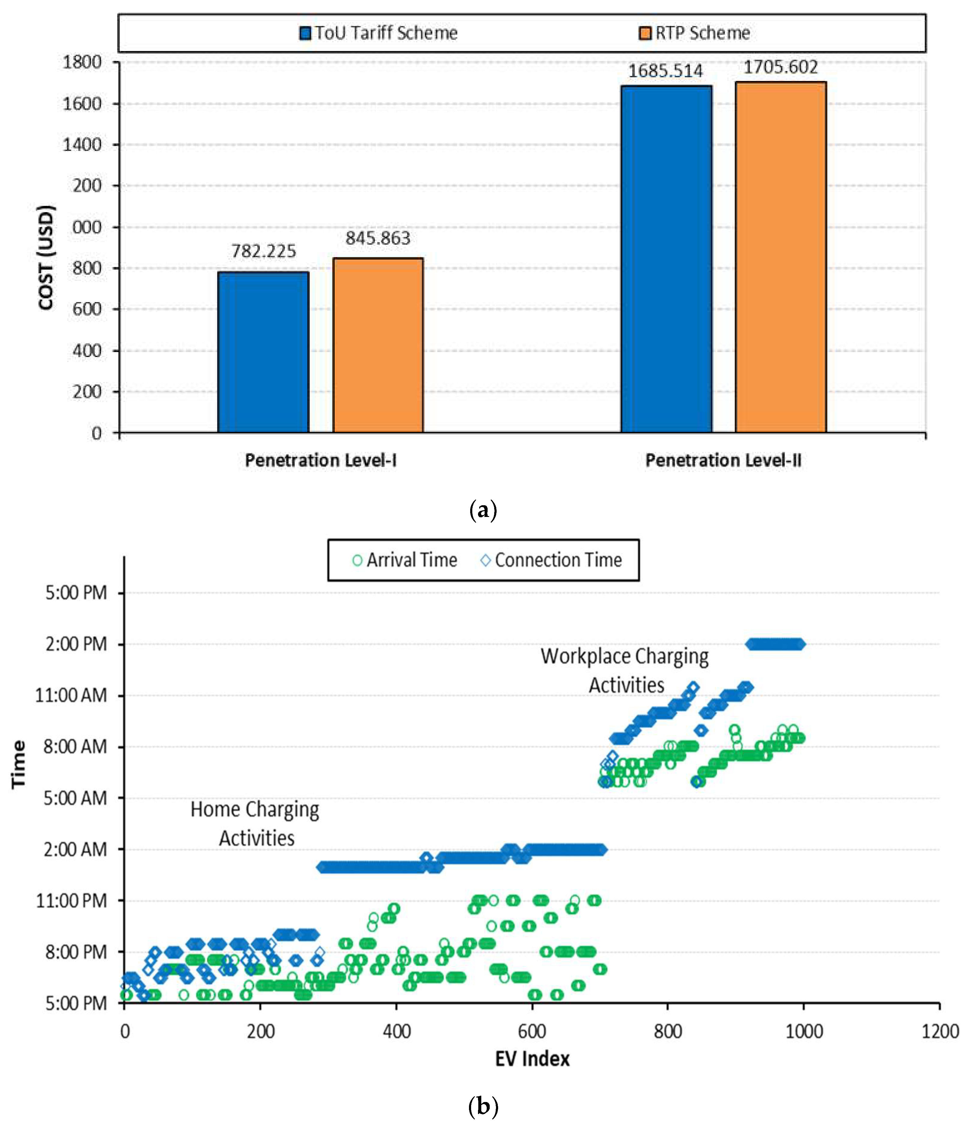
6.4. Case: D: Coordinated EV Charging with ToU and RTP Tariff for Both Waiting Time and Charging Cost Minimization
7. Comparison with the Reported Work
8. Conclusions
Author Contributions
Funding
Institutional Review Board Statement
Informed Consent Statement
Data Availability Statement
Conflicts of Interest
Abbreviations
| Nomenclature | |
| EVs | Electric Vehicles |
| PSO | Particle Swarm Optimization |
| DNO | Distribution Network Operator |
| GA | Genetic Algorithm |
| ToU | Time of Use |
| RTP | Real Time Pricing |
| SoC | State of Charge |
| AECM | Aggregator based EV charging Management |
| PLI | Power Loss Index |
| VDI | Voltage Deviation Index |
| CCI | Charging Cost Index |
| WTI | Waiting Time Index |
| BPSO | Binary Particle Swarm Optimization |
| BEP | Binary Evolutionary Programming |
| AHP | Analytic Hierarchy Process |
| BGWO | Binary Grey Wolf Optimization |
| WFA | Water Flow Algorithm |
| Math Symbols | |
| Power loss with charging power allocation | |
| Power loss without charging power allocation | |
| Simulation interval (30 min) | |
| Total simulation time (24 h) | |
| Current (A) through branch | |
| Resistance (ohm) of branch | |
| Total number of branches | |
| Reference voltage (p.u) | |
| Minimum voltage (p.u) recorded in time step | |
| Lower limit of voltage (p.u) at bus b | |
| Upper limit of voltage (p.u) at bus b | |
| Voltage (p.u) recorded at anu bus b in time step | |
| B | Total number of buses |
| Power allocation (kW) to the candidate aggregator a in time step | |
| Minimum power allocation (kW) to candidate aggregator a in time step | |
| Maximum power allocation (kW) to candidate aggregator a in time step | |
| A | Total number of aggregator agents |
| Instantaneous load demand (kW) at residential feeder s in time step | |
| Maximum residential load demand (kW) | |
| Instantaneous load demand (kW) at commercial feeder c in time step | |
| Maximum commercial load demand (kW) | |
| S | Total number of residential feeders |
| C | Total number of commercial feeders |
| Maximum load demand at the grid station (kW) | |
| Charging power (kW) of eth EV operation under agent a in a time step | |
| Charging cost in a time step (USD) | |
| Incentive for CO2 emission reduction | |
| Total time slots | |
| Set of EVs | |
| Time interval when EV charging starts | |
| Time interval when EV charging ends | |
| Arrival time of eth EV belongs to ath aggregator agent | |
| Connection time of eth EV belongs to ath aggregator agent | |
| Stay time of eth EV belongs to ath aggregator agent | |
| Departure time of eth EV belongs to ath aggregator agent | |
| Time required to obtain requested SoC of eth EV belongs to ath aggregator agent | |
| Battery Capacity (kWh) of eth EV belongs to ath aggregator agent | |
| Requested state of charge of eth EV belongs to ath aggregator agent | |
| Arrival state of charge of eth EV belongs to ath aggregator agent | |
| Efficiency of eth EV’s charger belongs to ath aggregator agent | |
| Charger rating (kW) of eth EV belongs to ath aggregator agent | |
References
- Yong, J.Y.; Ramachandaramurthy, V.K.; Tan, K.M.; Mithulananthan, N. A review on the state-of-the-art technologies of electric vehicle, its impacts and prospects. Renew. Sustain. Energy Rev. 2015, 49, 365–385. [Google Scholar] [CrossRef]
- Mozafar, M.R.; Amini, M.H.; Moradi, M.H. Innovative appraisement of smart grid operation considering large-scale integration of electric vehicles enabling V2G and G2V systems. Electr. Power Syst. Res. 2018, 154, 245–256. [Google Scholar] [CrossRef]
- Ul-Haq, A.; Cecati, C.; Strunz, K.; Abbasi, E. Impact of electric vehicle charging on voltage unbalance in an urban distribution network. Intell. Ind. Syst. 2015, 1, 51–60. [Google Scholar] [CrossRef] [Green Version]
- Yu, Y.; Reihs, D.; Wagh, S.; Shekhar, A.; Stahleder, D.; Mouli, G.R.C.; Lehfuss, F.; Bauer, P. Data-Driven Study of Low Voltage Distribution Grid Behaviour with Increasing Electric Vehicle Penetration. IEEE Access 2022, 10, 6053–6070. [Google Scholar] [CrossRef]
- Margossian, H.; Sayed, M.A.; Fawaz, W.; Nakad, Z. Partial grid false data injection attacks against state estimation. Int. J. Electr. Power Energy Syst. 2019, 110, 623–629. [Google Scholar] [CrossRef]
- Viel, F.; Augusto Silva, L.; Leithardt, V.R.Q.; De Paz Santana, J.F.; Celeste Ghizoni Teive, R.; Albenes Zeferino, C. An Efficient Interface for the Integration of IoT Devices with Smart Grids. Sensors 2020, 20, 2849. [Google Scholar] [CrossRef] [PubMed]
- Ullah, N. Electric Vehicles in Pakistan: Policy Recommendations; LUMS Energy Institute: Lahore, Pakistan, 2019; p. 43. [Google Scholar]
- Board, C.A.R. California’s Advanced Clean Cars Midterm Review; California Air Resources Board Sacramento: Sacramento, CA, USA, 2017. [Google Scholar]
- Basma, H.; Haddad, M.; Mansour, C.; Nemer, M.; Stabat, P. Assessing the charging load of battery electric bus fleet for different types of charging infrastructure. In Proceedings of the 2021 IEEE Transportation Electrification Conference & Expo (ITEC), Chicago, IL, USA, 21–25 June 2021; pp. 887–892. [Google Scholar]
- Kuppusamy, P.; Kumari, N.M.J.; Alghamdi, W.Y.; Alyami, H.; Ramalingam, R.; Javed, A.R.; Rashid, M. Job scheduling problem in fog-cloud-based environment using reinforced social spider optimization. J. Cloud Comput. 2022, 11, 99. [Google Scholar] [CrossRef]
- Amin, A.; Tareen, W.U.K.; Usman, M.; Memon, K.A.; Horan, B.; Mahmood, A.; Mekhilef, S. An integrated approach to optimal charging scheduling of electric vehicles integrated with improved medium-voltage network reconfiguration for power loss minimization. Sustainability 2020, 12, 9211. [Google Scholar] [CrossRef]
- Usman, M.; Tareen, W.U.K.; Amin, A.; Ali, H.; Bari, I.; Sajid, M.; Seyedmahmoudian, M.; Stojcevski, A.; Mahmood, A.; Mekhilef, S. A coordinated charging scheduling of electric vehicles considering optimal charging time for network power loss minimization. Energies 2021, 14, 5336. [Google Scholar] [CrossRef]
- Suyono, H.; Rahman, M.T.; Mokhlis, H.; Othman, M.; Illias, H.A.; Mohamad, H. Optimal scheduling of plug-in electric vehicle charging including time-of-use tariff to minimize cost and system stress. Energies 2019, 12, 1500. [Google Scholar] [CrossRef] [Green Version]
- Khan, S.U.; Mehmood, K.K.; Haider, Z.M.; Rafique, M.K.; Kim, C.-H. A bi-level EV aggregator coordination scheme for load variance minimization with renewable energy penetration adaptability. Energies 2018, 11, 2809. [Google Scholar] [CrossRef] [Green Version]
- Islam, J.B.F.; Rahman, M.T.; Mokhlis, H.; Othman, M.; IZAM, T.F.T.M.N.; Mohamad, H. Combined analytic hierarchy process and binary particle swarm optimization formultiobjective plug-in electric vehicles charging coordination with time-of-usetariff. Turk. J. Electr. Eng. Comput. Sci. 2020, 28, 1314–1330. [Google Scholar] [CrossRef]
- Khan, S.U.; Mehmood, K.K.; Haider, Z.M.; Rafique, M.K.; Khan, M.O.; Kim, C.-H. Coordination of multiple electric vehicle aggregators for peak shaving and valley filling in distribution feeders. Energies 2021, 14, 352. [Google Scholar] [CrossRef]
- Mohamed, N.M.M.; Sharaf, H.M.; Ibrahim, D.K. Proposed Ranked Strategy for Technical and Economical Enhancement of EVs Charging with High Penetration Level. IEEE Access 2022, 10, 44738–44755. [Google Scholar] [CrossRef]
- Xia, M.; Liao, T.; Chen, Q. Two-layer optimal charging strategy for electric vehicles in old residential areas. Int. Trans. Electr. Energy Syst. 2021, 31, e12890. [Google Scholar] [CrossRef]
- Fridgen, G.; Thimmel, M.; Weibelzahl, M.; Wolf, L. Smarter charging: Power allocation accounting for travel time of electric vehicle drivers. Transp. Res. D Transp. Environ. 2021, 97, 102916. [Google Scholar] [CrossRef]
- Yilmaz, M.; Krein, P.T. Review of battery charger topologies, charging power levels, and infrastructure for plug-in electric and hybrid vehicles. IEEE Trans. Power Electron. 2012, 28, 2151–2169. [Google Scholar] [CrossRef]
- ElCheikh, A.; ElKhoury, M. Effect of local grid refinement on performance of scale-resolving models for simulation of complex external flows. Aerospace 2019, 6, 86. [Google Scholar] [CrossRef] [Green Version]
- Power, W. What Is Peak Demand? Available online: https://www.westernpower.com.au/faqs/connect-to-the-network/what-is-peak-demand/what-is-peak-demand/ (accessed on 1 February 2023).
- Energy, B.P. What Is Peak Load Management? Available online: https://bestpracticeenergy.com/2020/04/07/peak-load-management/ (accessed on 1 February 2023).
- Injeti, S.K.; Thunuguntla, V.K. Optimal integration of DGs into radial distribution network in the presence of plug-in electric vehicles to minimize daily active power losses and to improve the voltage profile of the system using bio-inspired optimization algorithms. Prot. Control Mod. 2020, 5, 1–15. [Google Scholar] [CrossRef] [Green Version]
- Shin, H.; Baldick, R. Plug-in electric vehicle to home (V2H) operation under a grid outage. IEEE Trans. Smart Grid 2016, 8, 2032–2041. [Google Scholar] [CrossRef]
- Chai, S.; Xu, N.Z.; Niu, M.; Chan, K.W.; Chung, C.Y.; Jiang, H.; Sun, Y. An Evaluation Framework for Second-Life EV/PHEV Battery Application in Power Systems. IEEE Access 2021, 9, 152430–152441. [Google Scholar] [CrossRef]
- Lee, J.H.; Chakraborty, D.; Hardman, S.J.; Tal, G. Exploring electric vehicle charging patterns: Mixed usage of charging infrastructure. Transp. Res. Part D Transp. Environ. 2020, 79, 102249. [Google Scholar] [CrossRef]
- Guerrero, J.; Chapman, A.; Verbic, G. A study of energy trading in a low-voltage network: Centralised and distributed approaches. In Proceedings of the 2017 Australasian Universities Power Engineering Conference (AUPEC), Melbourne, Australia, 19–22 November 2017; pp. 1–6. [Google Scholar]
- Ahmed, E.M.; Rathinam, R.; Dayalan, S.; Fernandez, G.S.; Ali, Z.M.; Abdel Aleem, S.H.; Omar, A.I. A comprehensive analysis of demand response pricing strategies in a smart grid environment using particle swarm optimization and the strawberry optimization algorithm. Mathematics 2021, 9, 2338. [Google Scholar] [CrossRef]


| Ref. | EV Charging Control Architecture | Research Objectives | Optimization Method | Charging Platform | Pricing Scheme |
|---|---|---|---|---|---|
| [11] | Centralized | Power loss minimization | Binary PSO | Residential | Not applicable |
| [12] | Centralized | Power loss minimization | Binary EP | Residential | Not applicable |
| [13] | Centralized | Cost and system stress minimization | Binary PSO | Residential | ToU |
| [14] | Hierarchal | Peak shaving and valley filling | Water-filling algorithm | Residential | Not applicable |
| [15] | Centralized | Power loss and charging cost minimization | Binary PSO and analytical hierarchy process | Residential | ToU |
| [16] | Hierarchal | Peak shaving and valley filling | Heuristic | Residential | Not applicable |
| [17] | Centralized | Peak power, power losses and cost minimization | PSO | Residential | RTP |
| [18] | Hierarchal | Electricity distribution and charging schedule optimization | PSO | Residential | ToU |
| Proposed | Hierarchically centralized | Power loss, voltage deviation, charging cost and waiting time minimization | PSO, GA | Residential, Commercial | ToU and RTP |
| Battery Capacity [13,25,26] | Charger Rating [13] | Number of EVs | Residential Charging Fleet [27] | Workplace Charging Fleet [27] | Common Charging Fleet [27] | |
|---|---|---|---|---|---|---|
| Penetration I | Penetration II | |||||
| 10.5 kWh | 3.3 kW | 176 | 352 | 53% | 14% | 33% |
| 19.2 kWh | 6.6 kW | 164 | 328 | |||
| 20.7 kWh | 7.2 kW | 156 | 312 | |||
| Case No. | Description | Tariff Scheme | Waiting Time Minimization | Charging Cost Minimization | |
|---|---|---|---|---|---|
| ToU | RTP | ||||
| A | Uncoordinated EV Charging | √ | √ | √ | √ |
| B | Coordinated EV charging with ToU and RTP tariff for waiting time minimization | √ | √ | √ | O |
| C | Coordinated EV Charging with ToU and RTP tariff for charging cost minimization | √ | √ | O | √ |
| D | Coordinated EV Charging with ToU and RTP tariff for both waiting time and charging cost minimization | √ | √ | √ | √ |
| Performance Parameters | EV Penetration Levels | Cases | |||
|---|---|---|---|---|---|
| A | B | C | D | ||
| Total Power Loss (kW) | Level-I | 6562.9858 | 6266.4944 | 6249.5636 | 6191.5129 |
| Level-II | 7150.0197 | 6591.8251 | 6509.6295 | 6495.0645 | |
| Power Loss Index (%) | Level-I | 7.6933 | 3.3259 | 3.0640 | 2.1551 |
| Level-II | 15.2719 | 8.0971 | 6.9367 | 6.7280 | |
| Min. Voltage (p.u) | Level-I | 0.8931 | 0.9024 | 0.9320 | 0.9028 |
| Level-II | 0.8862 | 0.9010 | 0.9301 | 0.9023 | |
| Voltage Deviation Index (%) | Level-I | 7.9199 | 7.5421 | 7.5430 | 7.5633 |
| Level-II | 8.6309 | 7.9238 | 7.8584 | 7.8787 | |
| Performance Parameters | EV Penetration Levels | Cases | ||||
|---|---|---|---|---|---|---|
| A | B | C | D | |||
| Total Charging Cost (USD) | ToU | Level-I | 1482.09 | 1097.67 | 618.588 | 782.22 |
| RTP | Level-I | 1340.09 | 1028.46 | 770.0326 | 845.86 | |
| ToU | Level-II | 2964.19 | 2303.00 | 1388.34 | 1685.5 | |
| RTP | Level-II | 2680.18 | 1974.67 | 1561.5171 | 1705.60 | |
| Charging Cost Index (%) | ToU | Level-I | 30.88 | 22.86 | 12.88 | 16.29 |
| RTP | Level-I | 27.92 | 21.42 | 16.04 | 17.62 | |
| ToU | Level-II | 61.75 | 47.97 | 28.92 | 35.11 | |
| RTP | Level-II | 55.84 | 41.13 | 32.53 | 35.53 | |
| Average Waiting Time (Hr.) | Level-I | 0 | 1 | 2.5 | 1.5 | |
| Level-II | 0 | 1.5 | 3 | 2 | ||
| Waiting Time Index (%) | Level-I | 0 | 3 | 7.55 | 3.55 | |
| Level-II | 0 | 3.75 | 12 | 4.25 | ||
| Case No. | EV Penetration Levels | Charging Cost Index | Waiting Time Index | Overall Charging Satisfaction Index | ||
|---|---|---|---|---|---|---|
| ToU | RTP | ToU | RTP | |||
| A | Level-I | 30.88 | 27.92 | 0 | 69.12 | 72.08 |
| Level-II | 61.75 | 55.84 | 0 | 38.25 | 44.16 | |
| B | Level-I | 22.86 | 21.42 | 3 | 74.14 | 75.58 |
| Level-II | 47.97 | 41.13 | 3.75 | 48.28 | 55.12 | |
| C | Level-I | 12.88 | 16.04 | 7.55 | 79.57 | 76.41 |
| Level-II | 28.92 | 32.53 | 12 | 59.08 | 55.47 | |
| D | Level-I | 16.29 | 17.62 | 3.55 | 80.16 | 78.83 |
| Level-II | 35.11 | 35.53 | 4.25 | 60.64 | 60.22 | |
| Ref. | Objectives | Techniques Applied | Different Charging Platforms | Customer Satisfaction | Multi-Agent-Based Control of Charging Activities | ||
|---|---|---|---|---|---|---|---|
| Home | Workplace | Cost | Early Charging | ||||
| [11] | Power loss minimization | BPSO | √ | O | O | O | O |
| [12] | Power loss minimization | BEP | √ | O | O | O | O |
| [15] | Power loss minimization, charging cost minimization | BPSO and AHP | √ | O | √ | O | O |
| [13] | Cost and system stress minimization | BPSO and BGWO | √ | O | √ | O | O |
| [14] | Load variance minimization | WFA | √ | O | O | O | √ |
| [16] | Peak shaving and valley filling | Heuristic approach | √ | O | O | O | √ |
| Proposed work | Minimization of power loss, voltage deviation, charging cost and waiting time | PSO and GA | √ | √ | √ | √ | √ |
Disclaimer/Publisher’s Note: The statements, opinions and data contained in all publications are solely those of the individual author(s) and contributor(s) and not of MDPI and/or the editor(s). MDPI and/or the editor(s) disclaim responsibility for any injury to people or property resulting from any ideas, methods, instructions or products referred to in the content. |
© 2023 by the authors. Licensee MDPI, Basel, Switzerland. This article is an open access article distributed under the terms and conditions of the Creative Commons Attribution (CC BY) license (https://creativecommons.org/licenses/by/4.0/).
Share and Cite
Amin, A.; Mahmood, A.; Khan, A.R.; Arshad, K.; Assaleh, K.; Zoha, A. A Two-Stage Multi-Agent EV Charging Coordination Scheme for Maximizing Grid Performance and Customer Satisfaction. Sensors 2023, 23, 2925. https://doi.org/10.3390/s23062925
Amin A, Mahmood A, Khan AR, Arshad K, Assaleh K, Zoha A. A Two-Stage Multi-Agent EV Charging Coordination Scheme for Maximizing Grid Performance and Customer Satisfaction. Sensors. 2023; 23(6):2925. https://doi.org/10.3390/s23062925
Chicago/Turabian StyleAmin, Adil, Anzar Mahmood, Ahsan Raza Khan, Kamran Arshad, Khaled Assaleh, and Ahmed Zoha. 2023. "A Two-Stage Multi-Agent EV Charging Coordination Scheme for Maximizing Grid Performance and Customer Satisfaction" Sensors 23, no. 6: 2925. https://doi.org/10.3390/s23062925