


Exact and Heuristic Multi-Robot Dubins Coverage Path Planning for Known Environments
 ,
, 
Abstract
:1. Introduction
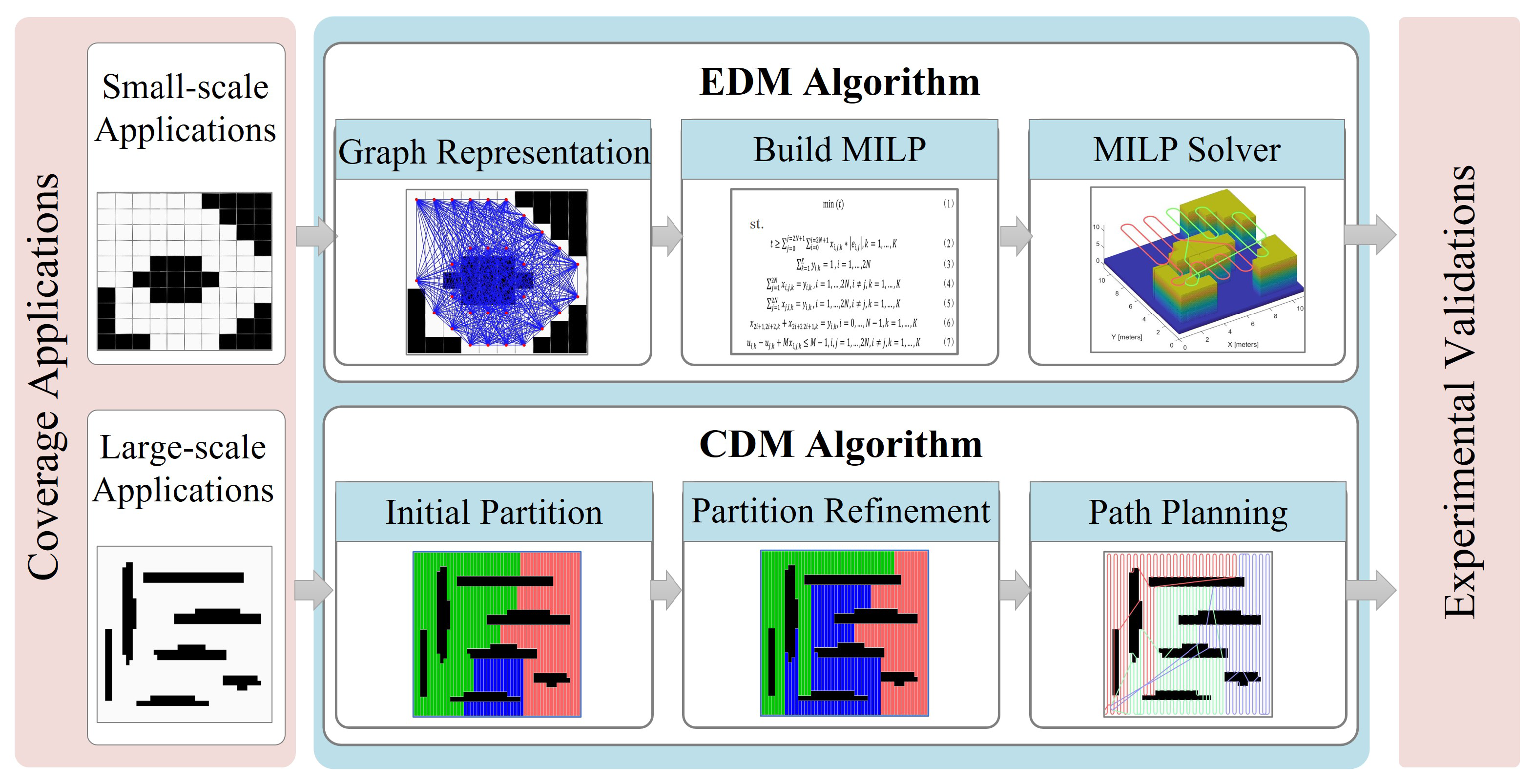
- We present an EDM algorithm based on MILP, which provides the shortest Dubins coverage path by searching the entire solution space.
- We present a CDM algorithm, which ensures the task balance among robots by the credit model and reduces complexity by a tree-partition strategy.
- Extensive validations. (i) Comparison experiments with other exact and heuristic MCPP methods show that EDM provides the minimum coverage time in small coverage scenes, and CDM generates a shorter coverage time and less computation time in large coverage scenes. (ii) Feasibility experiments are conducted on a high-fidelity UAV model to validate the applicability of EDM and CDM.
2. Related Work
2.1. Exact and Heuristic MCPP Methods
2.2. Dubins Coverage
3. System Overview
3.1. Problem Statement
3.2. System Overview
4. Exact Dubin Multi-Robot CPP (EDM) Algorithm
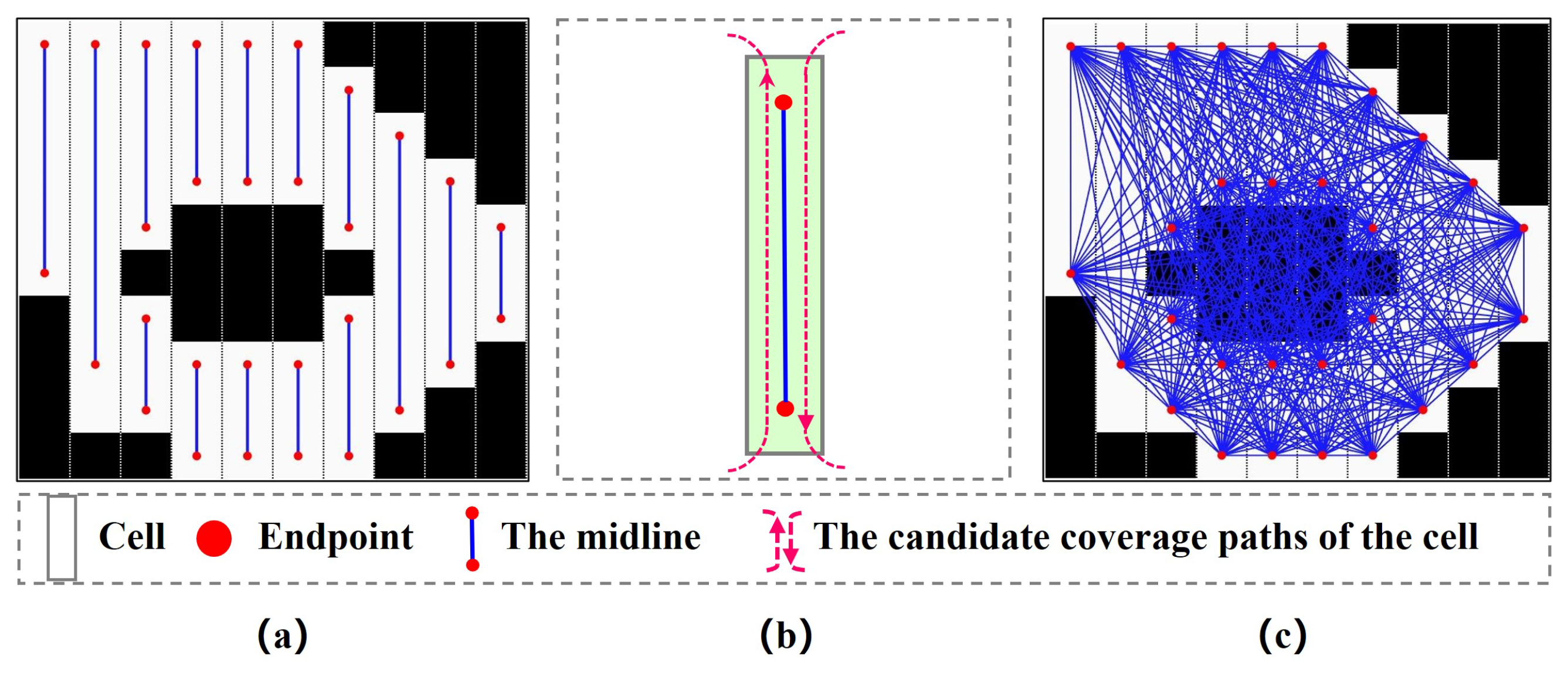
4.1. Graph Representation
4.2. Build MILP
4.3. Pseudo-Code of the EDM Algorithm
| Algorithm 1 EDM Algorithm |
| Input: , |
| Output: |
| 1: Initialize: ; |
| 2: Area_Decomposition(); |
| 3: Graph_Representation(); |
| 4: calculate the cost between points in G |
| 5: Build_MILP(G); // Equations (1)–(7) |
| 6: MILP_Solver; |
| 7: Dubins_Solver(); |
| 8: return |
5. Heuristic Credit-Based Dubin Multi-Robot CPP(CDM) Algorithm
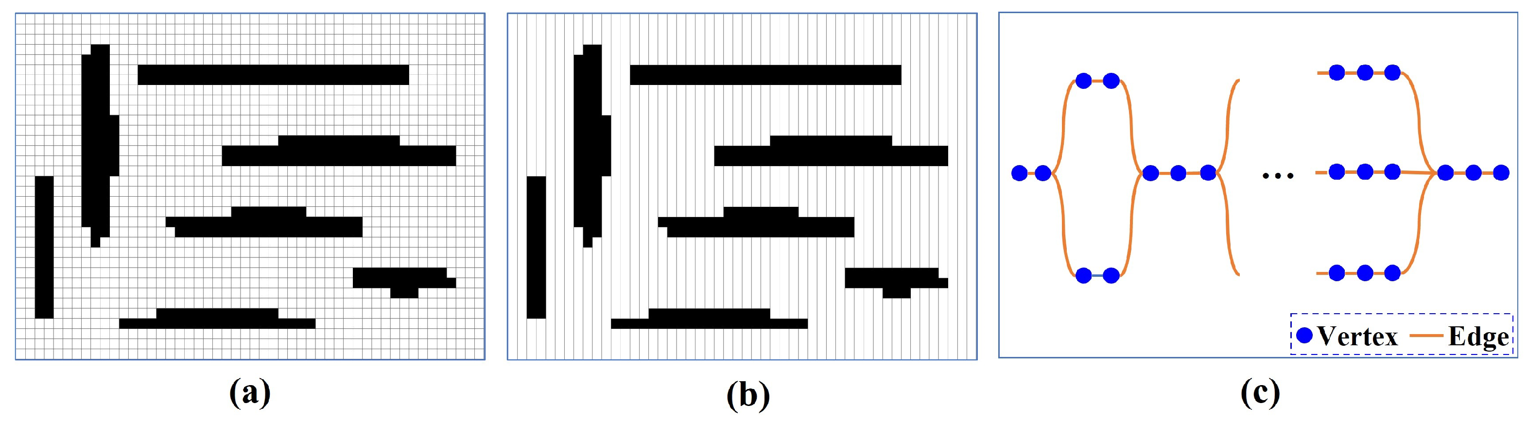
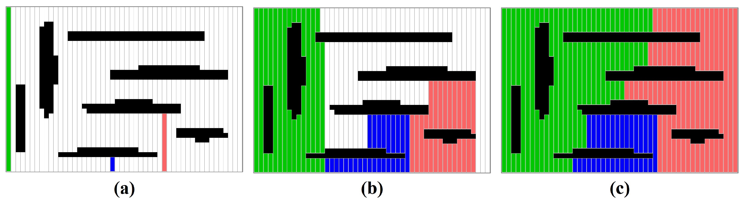
5.1. Initial Partition
5.2. Partition Refinement
5.3. Path Planning
5.4. Pseudo-Code of the CDM Algorithm
| Algorithm 2 CDM Algorithm |
| Input: , |
| Parameter: : The maximum number of task transactions |
| Output: |
| 1: Initialize: ; |
| 2: Area_Decomposition(); |
| 3: Graph_Representation(); |
| 4: initial_partition(); |
| 5: ; |
| 6: while do |
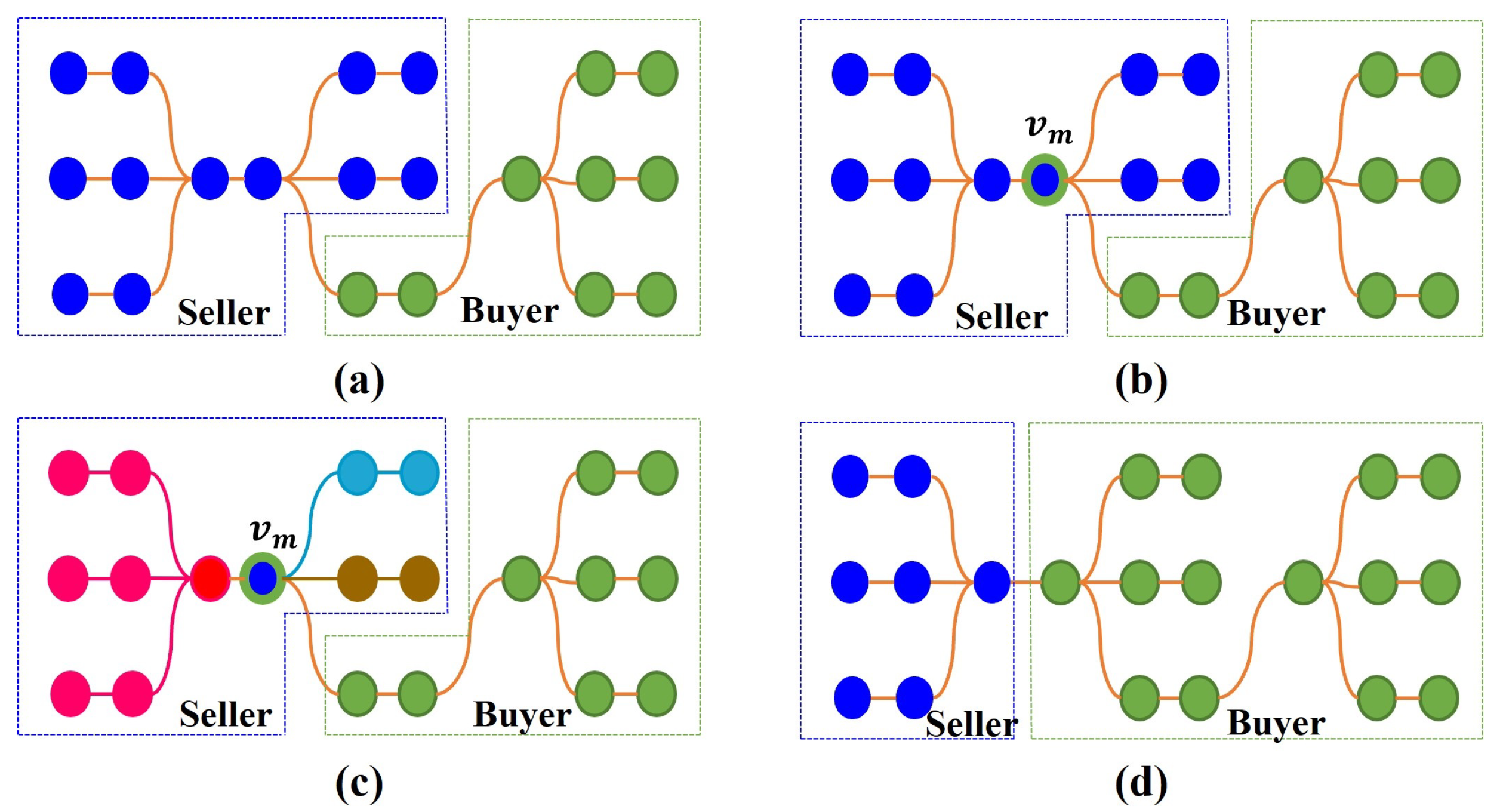
| 7: determine the seller and the buyer; |
| 8: calculate the set of adjacent cells between and ; |
| 9: ; |
| 10: for each in do |
| 11: tree_partition(); |
| 12: if then |
| 13: Trade tasks ; |
| 14: Update ; |
| 15: ; |
| 16: break; |
| 17: end if |
| 18: end for |
| 19: if then |
| 20: Mark and as a pair of non-tradable partitions. |
| 21: end if |
| 22: ; |
| 23: end while |
| 24: Dubins_Solver(); |
| 25: return; |
6. Experiments
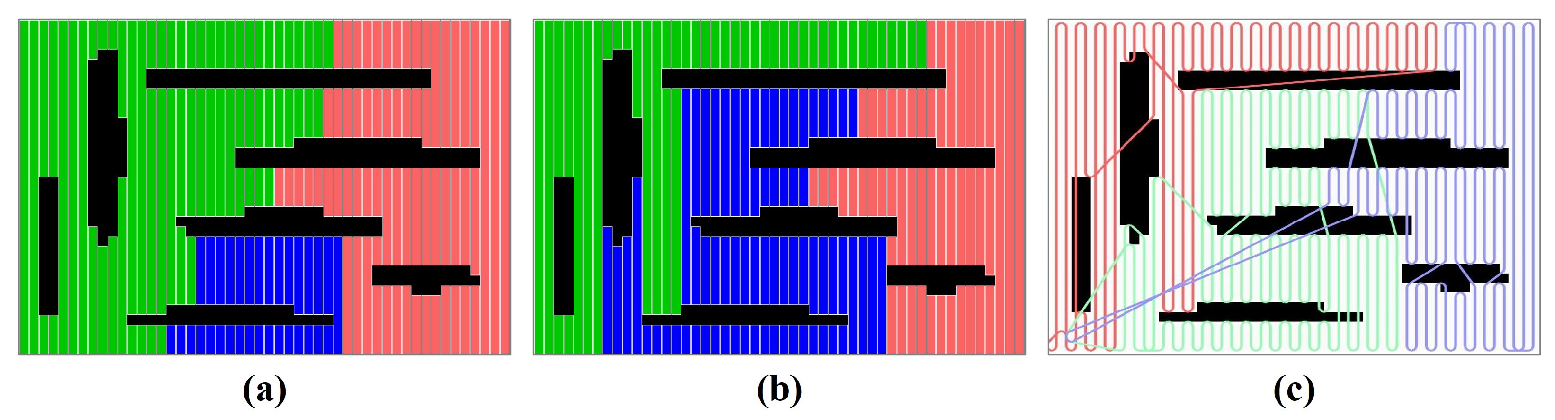
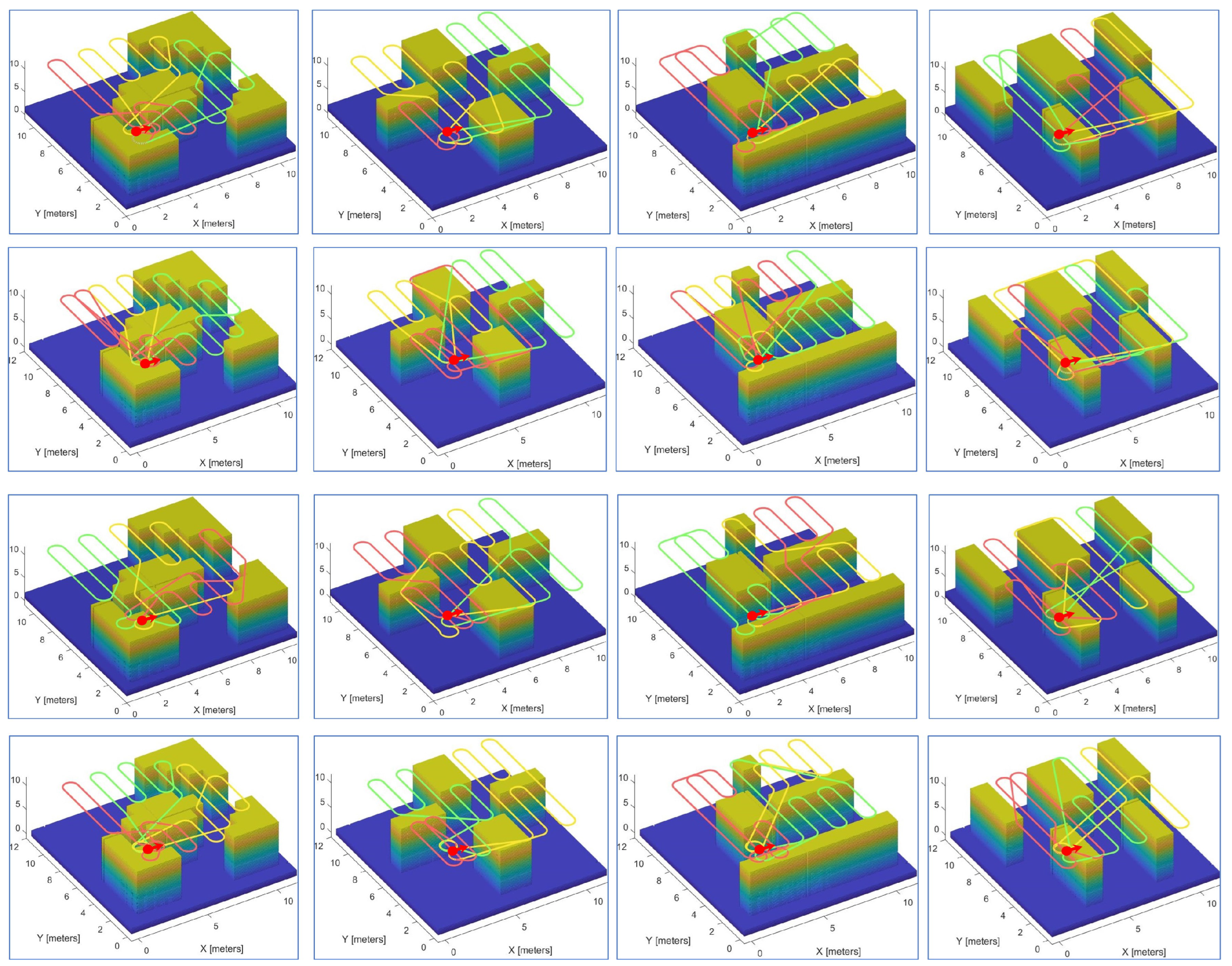
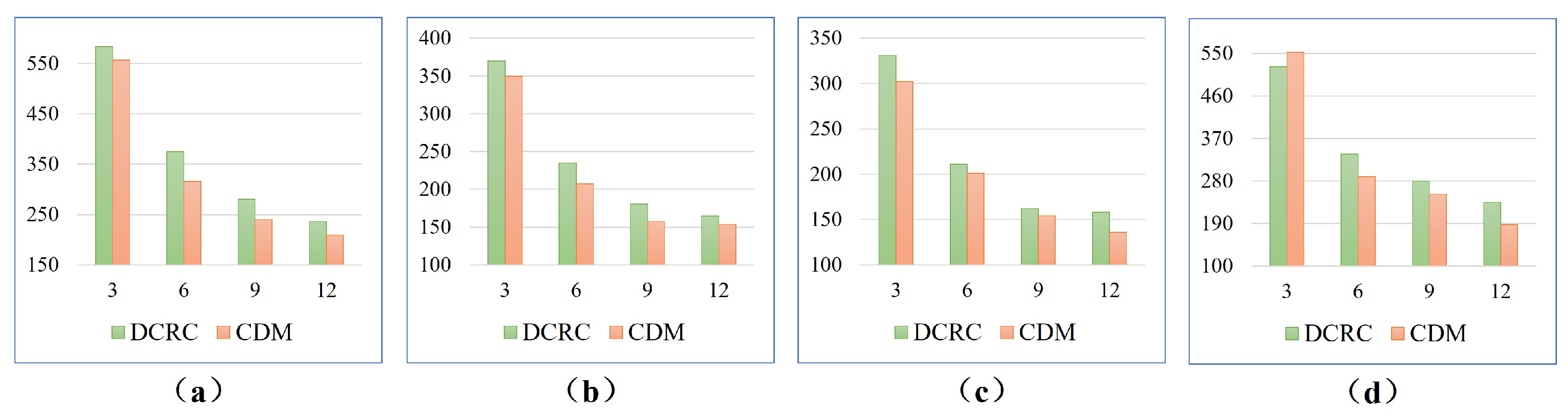
6.1. Comparison Experiments in Small Scenes
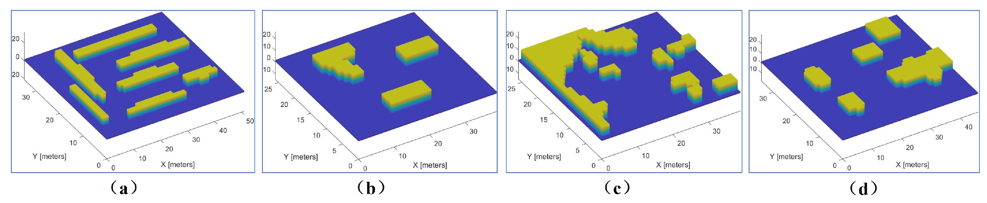
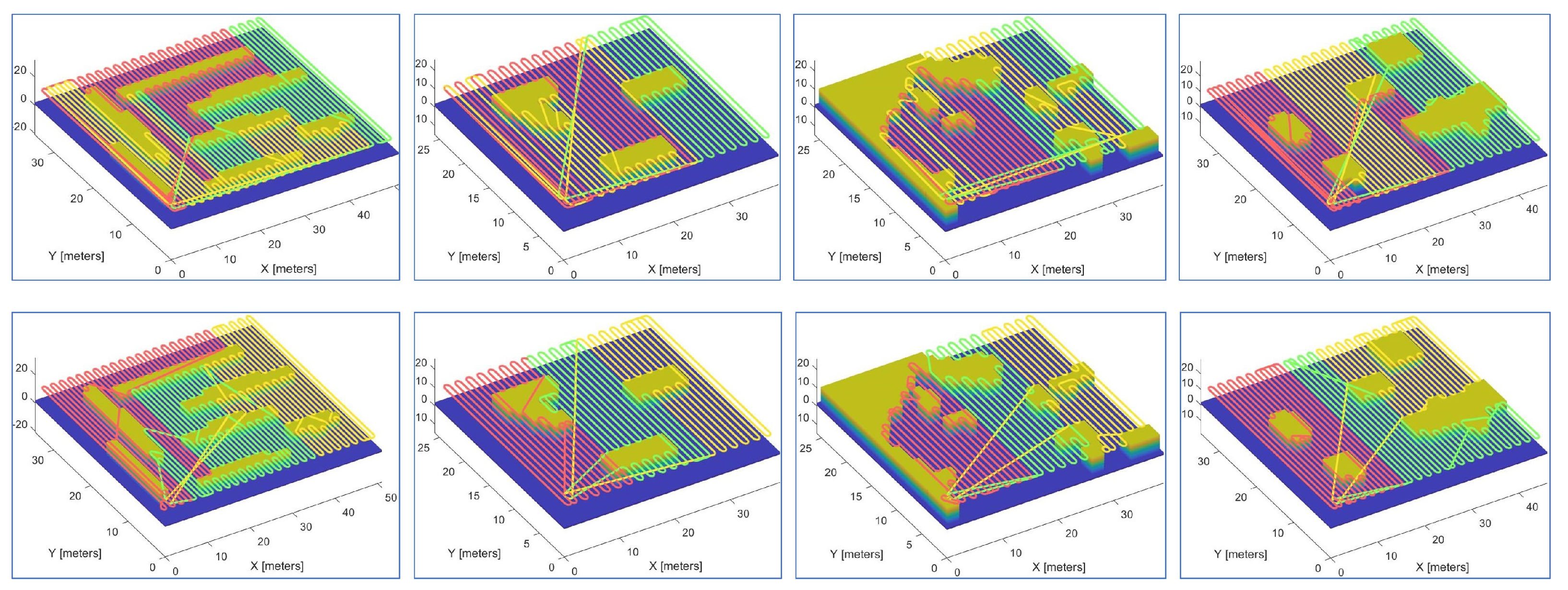
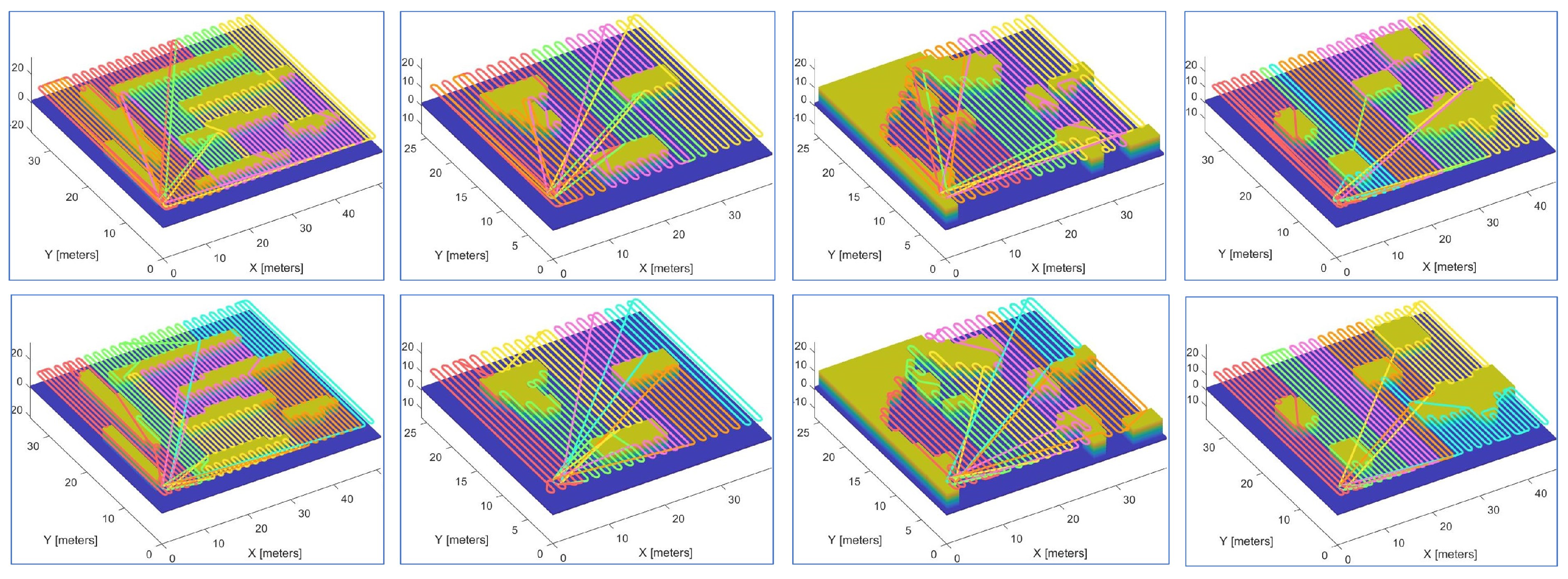
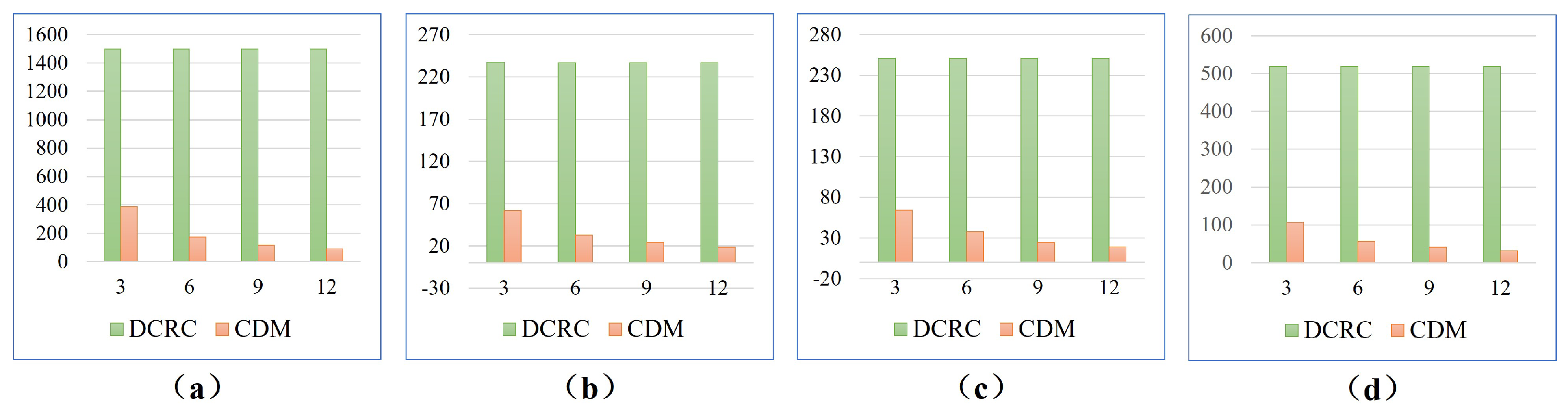
6.2. Comparison Experiments in Large Scenes
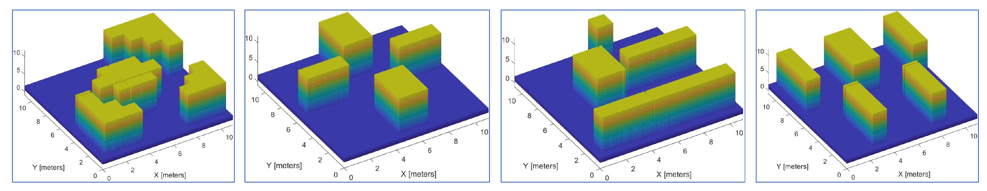
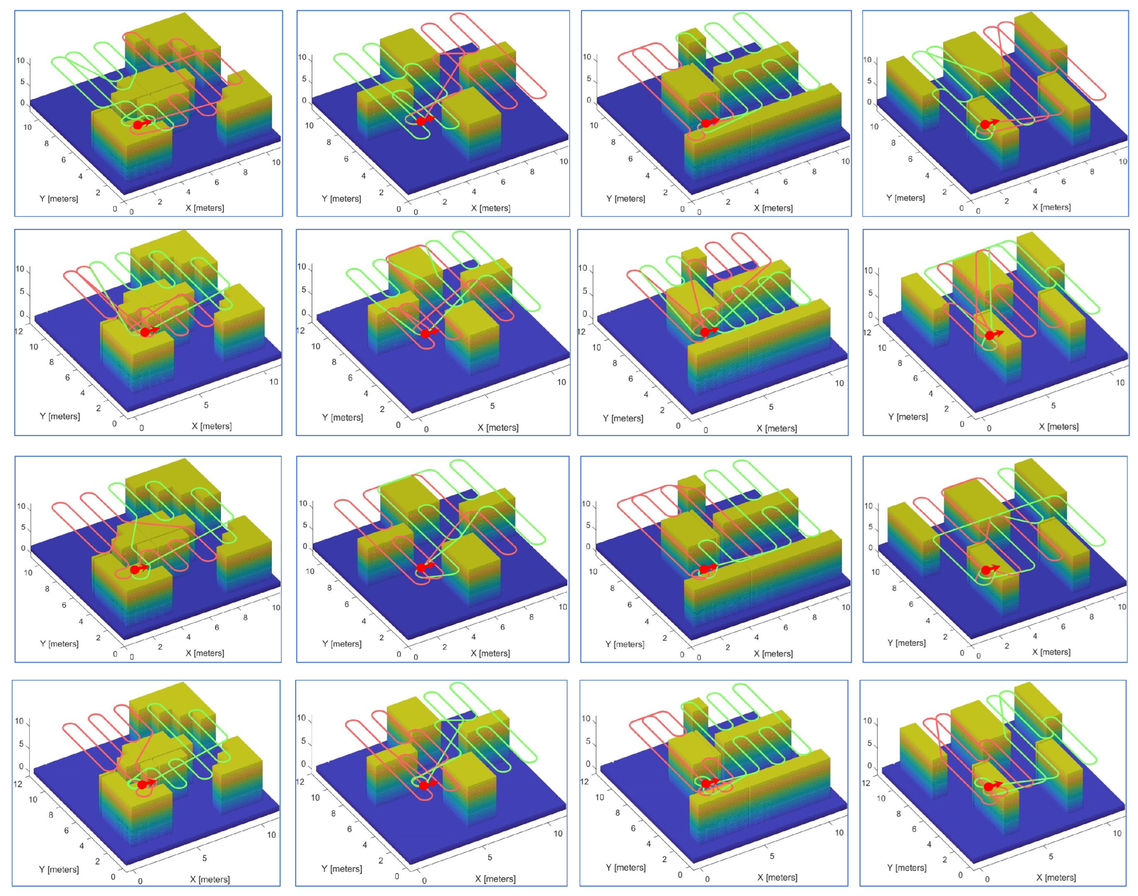
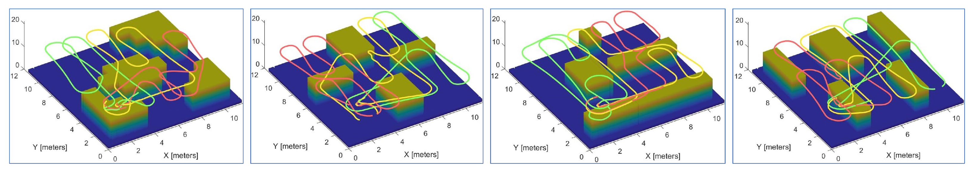
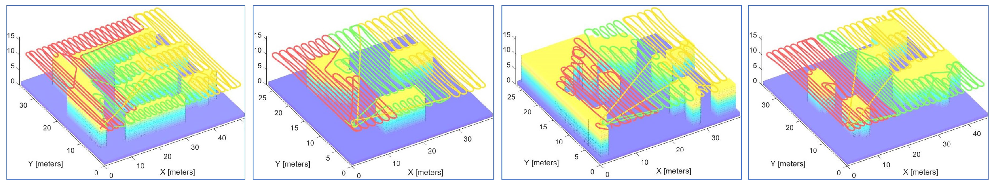
6.3. Feasibility Experiments of EDM and CDM
7. Conclusions
Author Contributions
Funding
Institutional Review Board Statement
Informed Consent Statement
Data Availability Statement
Acknowledgments
Conflicts of Interest
References
- Chen, J.; Ling, F.; Zhang, Y.; You, T.; Liu, Y.; Du, X. Coverage path planning of heterogeneous unmanned aerial vehicles based on ant colony system. Swarm Evol. Comput. 2022, 69, 101005. [Google Scholar] [CrossRef]
- Fevgas, G.; Lagkas, T.; Argyriou, V.; Sarigiannidis, P. Coverage path planning methods focusing on energy efficient and cooperative strategies for unmanned aerial vehicles. Sensors 2022, 22, 1235. [Google Scholar] [CrossRef]
- Karapetyan, N.; Moulton, J.; Lewis, J.S.; Li, A.Q.; O’Kane, J.M.; Rekleitis, I. Multi-robot dubins coverage with autonomous surface vehicles. In Proceedings of the 2018 IEEE International Conference on Robotics and Automation (ICRA), Brisbane, Australia, 21–25 May 2018; pp. 2373–2379. [Google Scholar]
- Chen, J.; Du, C.; Zhang, Y.; Han, P.; Wei, W. A clustering-based coverage path planning method for autonomous heterogeneous UAVs. IEEE Trans. Intell. Transp. Syst. 2022, 23, 25546–25556. [Google Scholar] [CrossRef]
- Karapetyan, N.; Benson, K.; McKinney, C.; Taslakian, P.; Rekleitis, I. Efficient multi-robot coverage of a known environment. In Proceedings of the 2017 IEEE/RSJ International Conference on Intelligent Robots and Systems (IROS), Vancouver, BC, Canada, 24–28 September 2017; pp. 1846–1852. [Google Scholar]
- Coombes, M.; Chen, W.H.; Liu, C. Flight testing Boustrophedon coverage path planning for fixed wing UAVs in wind. In Proceedings of the 2019 International Conference on Robotics and Automation (ICRA), Montreal, QC, Canada, 20–24 May 2019; pp. 711–717. [Google Scholar]
- Wilson, J.P.; Mittal, K.; Gupta, S. Novel motion models for time-optimal risk-aware motion planning for variable-speed AUVs. In Proceedings of the OCEANS 2019 MTS/IEEE SEATTLE, Seattle, WA, USA, 27–31 October 2019; pp. 1–5. [Google Scholar]
- Maini, P.; Gonultas, B.M.; Isler, V. Online coverage planning for an autonomous weed mowing robot with curvature constraints. IEEE Robot. Autom. Lett. 2022, 7, 5445–5452. [Google Scholar] [CrossRef]
- Deng, D.; Jing, W.; Fu, Y.; Huang, Z.; Liu, J.; Shimada, K. Constrained heterogeneous vehicle path planning for large-area coverage. In Proceedings of the 2019 IEEE/RSJ International Conference on Intelligent Robots and Systems (IROS), Macau, China, 3–8 November 2019; pp. 4113–4120. [Google Scholar]
- Dubins, L.E. On curves of minimal length with a constraint on average curvature, and with prescribed initial and terminal positions and tangents. Am. J. Math. 1957, 79, 497–516. [Google Scholar] [CrossRef]
- Rekleitis, I.; New, A.P.; Rankin, E.S.; Choset, H. Efficient boustrophedon multi-robot coverage: An algorithmic approach. Ann. Math. Artif. Intell. 2008, 52, 109–142. [Google Scholar] [CrossRef] [Green Version]
- Tan, C.S.; Mohd-Mokhtar, R.; Arshad, M.R. A comprehensive review of coverage path planning in robotics using classical and heuristic algorithms. IEEE Access 2021, 9, 119310–119342. [Google Scholar] [CrossRef]
- Cabreira, T.M.; Brisolara, L.B.; Ferreira, P.R., Jr. Survey on coverage path planning with unmanned aerial vehicles. Drones 2019, 3, 4. [Google Scholar] [CrossRef] [Green Version]
- Aggarwal, S.; Kumar, N. Path planning techniques for unmanned aerial vehicles: A review, solutions, and challenges. Comput. Commun. 2020, 149, 270–299. [Google Scholar] [CrossRef]
- Yu, X.; Jin, S.; Shi, D.; Li, L.; Kang, Y.; Zou, J. Balanced multi-region coverage path planning for unmanned aerial vehicles. In Proceedings of the 2020 IEEE International Conference on Systems, Man, and Cybernetics (SMC), Toronto, ON, Canada, 11–14 October 2020; pp. 3499–3506. [Google Scholar]
- Khan, A.; Noreen, I.; Habib, Z. On Complete Coverage Path Planning Algorithms for Non-holonomic Mobile Robots: Survey and Challenges. J. Inf. Sci. Eng. 2017, 33, 101–121. [Google Scholar]
- Li, L.; Shi, D.; Jin, S.; Kang, Y.; Xue, C.; Zhou, X.; Liu, H.; Yu, X. Complete coverage problem of multiple robots with different velocities. Int. J. Adv. Robot. Syst. 2022, 19, 17298806221091685. [Google Scholar] [CrossRef]
- Chen, J.; Zhang, Y.; Wu, L.; You, T.; Ning, X. An adaptive clustering-based algorithm for automatic path planning of heterogeneous UAVs. IEEE Trans. Intell. Transp. Syst. 2021, 23, 16842–16853. [Google Scholar] [CrossRef]
- Rafael Marti, G.R. (Ed.) Exact and Heuristic Methods in Combinatorial Optimization; Springer: Berlin/Heidelberg, Germany, 2022. [Google Scholar]
- Zhou, X.; Wang, H.; Ding, B.; Hu, T.; Shang, S. Balanced connected task allocations for multi-robot systems: An exact flow-based integer program and an approximate tree-based genetic algorithm. Expert Syst. Appl. 2019, 116, 10–20. [Google Scholar] [CrossRef]
- Matić, D. A mixed integer linear programming model and variable neighborhood search for maximally balanced connected partition problem. Appl. Math. Comput. 2014, 237, 85–97. [Google Scholar] [CrossRef]
- Sundar, K.; Rathinam, S. Algorithms for heterogeneous, multiple depot, multiple unmanned vehicle path planning problems. J. Intell. Robot. Syst. 2017, 88, 513–526. [Google Scholar] [CrossRef]
- Vandermeulen, I.; Groß, R.; Kolling, A. Turn-minimizing multirobot coverage. In Proceedings of the 2019 International Conference on Robotics and Automation (ICRA), Montreal, QC, Canada, 20–24 May 2019; pp. 1014–1020. [Google Scholar]
- Yu, X.; Roppel, T.A.; Hung, J.Y. An optimization approach for planning robotic field coverage. In Proceedings of the IECON 2015-41st Annual Conference of the IEEE Industrial Electronics Society, Yokohama, Japan, 9–12 November 2015; pp. 4032–4039. [Google Scholar]
- ElGibreen, H.; Youcef-Toumi, K. Dynamic task allocation in an uncertain environment with heterogeneous multi-agents. Auton. Robot. 2019, 43, 1639–1664. [Google Scholar] [CrossRef]
- Gabriely, Y.; Rimon, E. Spanning-tree based coverage of continuous areas by a mobile robot. Ann. Math. Artif. Intell. 2001, 31, 77–98. [Google Scholar] [CrossRef]
- Hazon, N.; Kaminka, G.A. Redundancy, efficiency and robustness in multi-robot coverage. In Proceedings of the 2005 IEEE International Conference on Robotics and Automation, Barcelona, Spain, 18–22 April 2005; pp. 735–741. [Google Scholar]
- Zheng, X.; Jain, S.; Koenig, S.; Kempe, D. Multi-robot forest coverage. In Proceedings of the 2005 IEEE/RSJ International Conference on Intelligent Robots and Systems, Edmonton, AB, Canada, 2–6 August 2005; pp. 3852–3857. [Google Scholar]
- Zhou, X.; Wang, H.; Ding, B. How Many Robots are Enough: A Multi-Objective Genetic Algorithm for the Single-Objective Time-Limited Complete Coverage Problem. In Proceedings of the IEEE 2018 International Conference on Robotics and Automation (ICRA), Brisbane, Australia, 21–25 May 2018; pp. 2380–2387. [Google Scholar]
- Wang, X.; Jiang, P.; Li, D.; Sun, T. Curvature continuous and bounded path planning for fixed-wing UAVs. Sensors 2017, 17, 2155. [Google Scholar] [CrossRef] [PubMed]
- Šelek, A.; Seder, M.; Brezak, M.; Petrović, I. Smooth Complete Coverage Trajectory Planning Algorithm for a Nonholonomic Robot. Sensors 2022, 22, 9269. [Google Scholar] [CrossRef]
- Duckett, T.; Pearson, S.; Blackmore, S.; Grieve, B.; Chen, W.H.; Cielniak, G.; Cleaversmith, J.; Dai, J.; Davis, S.; Fox, C.; et al. Agricultural robotics: The future of robotic agriculture. arXiv 2018, arXiv:1806.06762. [Google Scholar]
- Xu, A.; Viriyasuthee, C.; Rekleitis, I. Optimal complete terrain coverage using an unmanned aerial vehicle. In Proceedings of the 2011 IEEE International Conference on Robotics and Automation, Shanghai, China, 9–13 May 2011; pp. 2513–2519. [Google Scholar]
- Yu, X. Optimization Approaches for a Dubins Vehicle in Coverage Planning Problem and Traveling Salesman Problems. Ph.D. Thesis, AUBURN Univerisity, Auburn, AL, USA, 2015. [Google Scholar]
- Lewis, J.S.; Edwards, W.; Benson, K.; Rekleitis, I.; O’Kane, J.M. Semi-boustrophedon coverage with a dubins vehicle. In Proceedings of the 2017 IEEE/RSJ International Conference on Intelligent Robots and Systems (IROS), Vancouver, BC, Canada, 24–28 September 2017; pp. 5630–5637. [Google Scholar]
- Miller, C.E.; Tucker, A.W.; Zemlin, R.A. Integer programming formulation of traveling salesman problems. J. ACM (JACM) 1960, 7, 326–329. [Google Scholar] [CrossRef]
- Bixby, B. The gurobi optimizer. Transp. Res. Part B 2007, 41, 159–178. [Google Scholar]
- Frieze, A.M.; Galbiati, G.; Maffioli, F. On the worst-case performance of some algorithms for the asymmetric traveling salesman problem. Networks 1982, 12, 23–39. [Google Scholar] [CrossRef]
- Romero, P. Simulink Drone Reference Application. 2022. Available online: https://github.com/mathworks/simulinkDrone\ReferenceApp/releases/tag/v2.1 (accessed on 19 December 2022).


Disclaimer/Publisher’s Note: The statements, opinions and data contained in all publications are solely those of the individual author(s) and contributor(s) and not of MDPI and/or the editor(s). MDPI and/or the editor(s) disclaim responsibility for any injury to people or property resulting from any ideas, methods, instructions or products referred to in the content. |
© 2023 by the authors. Licensee MDPI, Basel, Switzerland. This article is an open access article distributed under the terms and conditions of the Creative Commons Attribution (CC BY) license (https://creativecommons.org/licenses/by/4.0/).
Share and Cite
Li, L.; Shi, D.; Jin, S.; Yang, S.; Zhou, C.; Lian, Y.; Liu, H. Exact and Heuristic Multi-Robot Dubins Coverage Path Planning for Known Environments. Sensors 2023, 23, 2560. https://doi.org/10.3390/s23052560
Li L, Shi D, Jin S, Yang S, Zhou C, Lian Y, Liu H. Exact and Heuristic Multi-Robot Dubins Coverage Path Planning for Known Environments. Sensors. 2023; 23(5):2560. https://doi.org/10.3390/s23052560
Chicago/Turabian StyleLi, Lin, Dianxi Shi, Songchang Jin, Shaowu Yang, Chenlei Zhou, Yaoning Lian, and Hengzhu Liu. 2023. "Exact and Heuristic Multi-Robot Dubins Coverage Path Planning for Known Environments" Sensors 23, no. 5: 2560. https://doi.org/10.3390/s23052560