
A Systematic Review of Advanced Sensor Technologies for Non-Destructive Testing and Structural Health Monitoring

Abstract
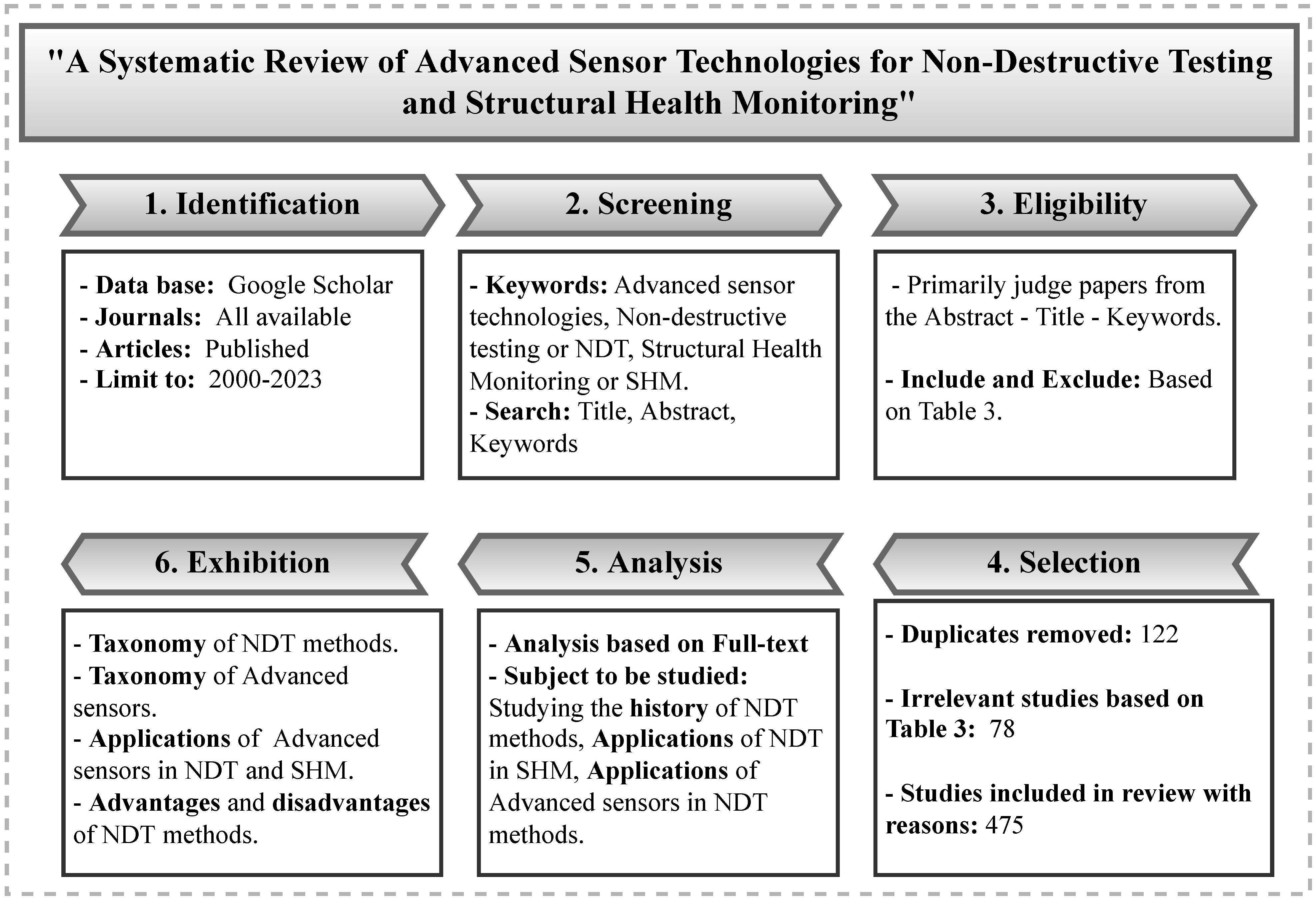
:1. Introduction
- We provide a detailed discussion on the relationship between NDT and SHM strategies, elaborating on differences and highlighting similarities.
- We present a comprehensive overview of various established and newly advanced NDT technologies discussing their advantages and disadvantages. We categorize NDT techniques into different groups providing application examples and the latest research studies. We provide detailed explanations of each method’s working principles, technical specifications, and recent innovations.
- We give an overview of SHM systems with details on methods, measurements, monitoring strategies, and technological benefits. We provide comprehensive information on conventional and advanced sensor technologies, including next-generation systems for SHM. We further address technologies for mitigating environmental and operational conditions (EOCs), such as temperature effects and their applications in SHM systems.
- We present recent advances and trends in signal processing, DL, ML, and AI used for NDT and SHM applications.
- Finally, future directions are discussed based on the knowledge acquired from this comprehensive review.
2. The Relationship between NDT and SHM Systems
- Sensor Network [54]: Sensing techniques used for NDT assessment typically have a high level of technological sophistication. In most cases, NDT techniques use only one type of sensor. It is common for NDT methods to be operated manually and applied following a standardized procedure. In general, NDT techniques are localized in nature, and they require an understanding of the location of the damage a priori. In SHM systems, on the other hand, a variety of sensors is utilized, and data transmission can be automated using a different transmission system, such as wireless communication networks. Large civil engineering structures benefit from SHM methods since they can cover large areas without needing prior knowledge of the damage location.
- System Identification [55]: SHM methods can be used to monitor a structure continuously and provide ongoing assessment information on the global status of the structure. Most SHM methods have the ability to incorporate system identification approaches and are appropriate for assessing modal and structural parameters. The reliable implementation of SHM-based system identification for large civil engineering structures is still an active field of research with developments in advanced sensing technology, data transfer systems, and data analytics. NDT techniques are not well suited to system identification since these methods evaluate local structural features rather than global behavior.
- Damage Diagnosis [56]: The use of NDT techniques can assist in identifying localized damage, provided that the area and type of damage are known before the damage is identified. Due to their localized nature, these techniques do not require global structural information and analytical models. The damage characteristics are often reliably predicted by NDT techniques using simple computational algorithms. SHM methods, on the other hand, allow for the global identification of structural damage. Identifying damage using SHM methods can be challenging, as they often require detailed structural geometry and material characteristics. A significant amount of computational effort may be required to identify SHM methods. Damage identification algorithms based on SHM are still under development to improve their reliability, accuracy, and efficiency.
- Damage Prognosis [57]: To make informed decisions, civil infrastructure management relies on damage prognosis methods that are precise and reliable. NDT methods can deliver accurate damage identification and assessment; however, due to their localized nature, they may not be able to provide reliable information on global damage characteristics and the overall structural system. Further, NDT techniques usually cannot model structural capacity and load conditions stochastically because of their short duration. SHM systems, on the other hand, are able to assess the performance of the entire structural system and provide global damage prognostics. Due to the availability of continuously monitored data, SHM methods can provide information for the stochastic modeling of structural systems for reliability analysis. Thereby, it is possible to determine the time-dependent reliability of the structure based on the evolution of the stochastic models.
3. NDT Systems
3.1. Conventional and Advanced NDT Techniques
3.1.1. Conventional NDT
3.1.2. Advanced NDT
3.2. NDT Categories
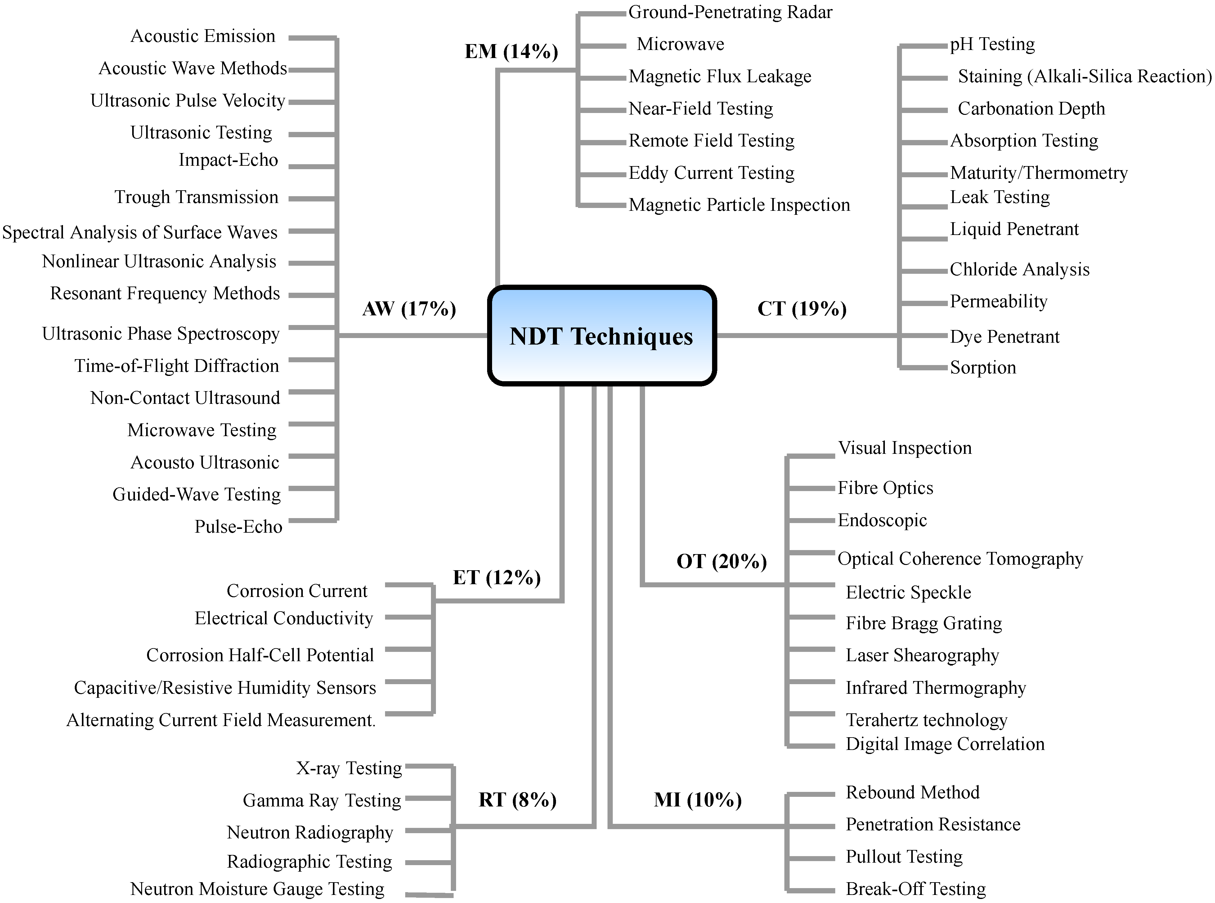
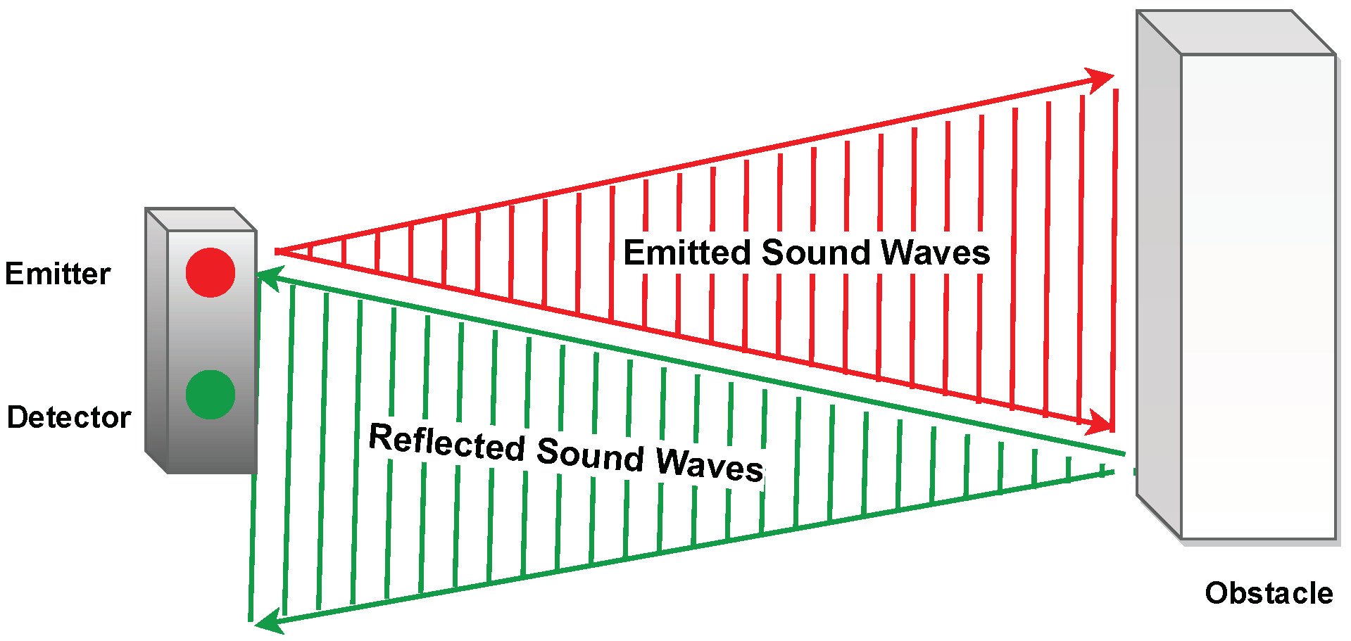
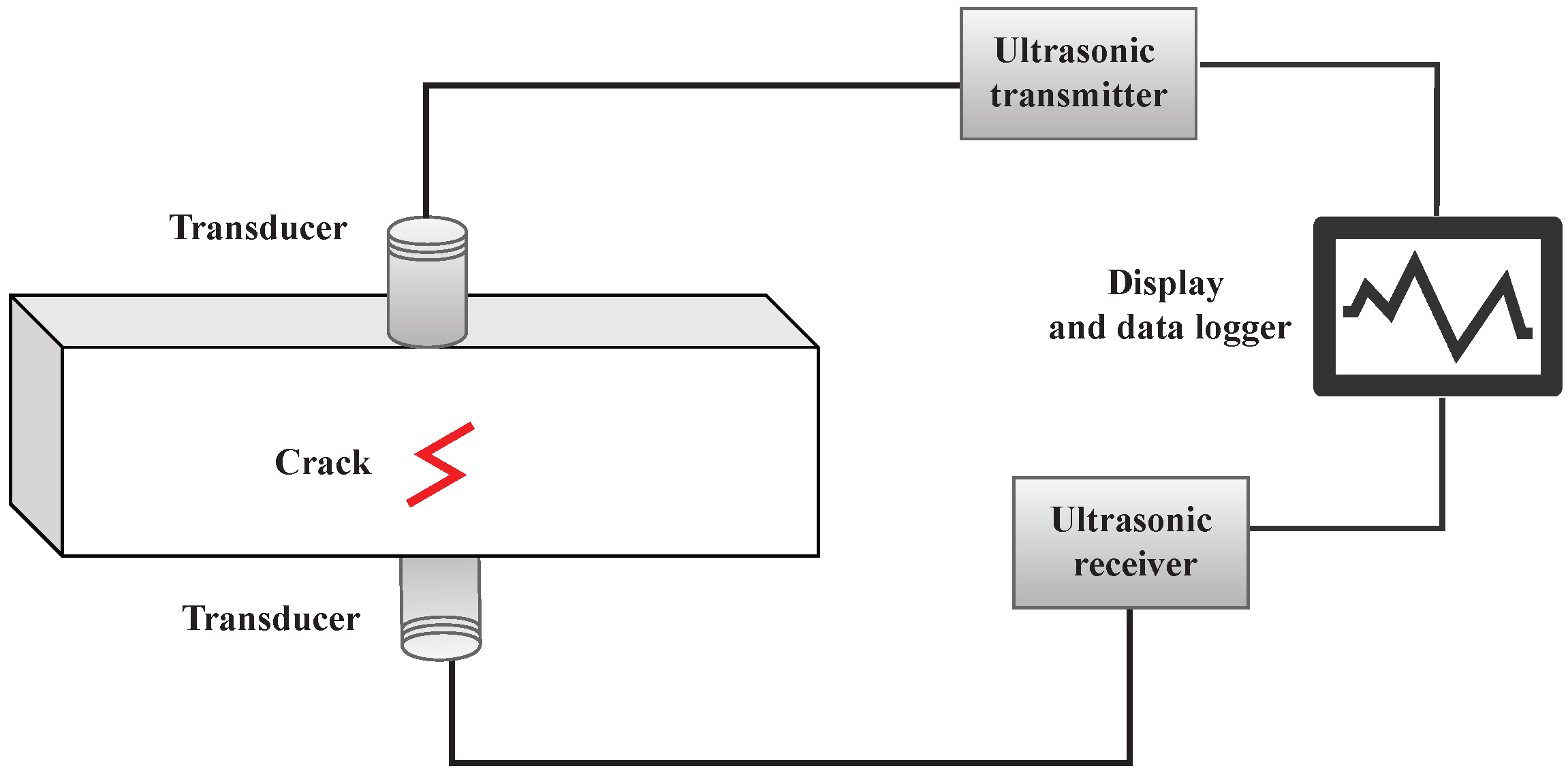
- Acoustic Wave Methods [117,118,119,120,121,122]: In acoustic wave methods, sonic and ultrasonic stress waves are detected and monitored. The stress waves are either passively emitted (such as in Acoustic Emission) or actively imparted (e.g., for Guided Wave Testing). They are typically conducted within the elastic material range in order to detect internal flaws and characterize materials. These methods include (1) Acoustic Emission, (2) Acoustic Wave Methods, (3) Ultrasonic Pulse Velocity (UPV), (4) Ultrasonic Testing, (5) Impact-Echo (IE), (6) Trough Transmission, (7) Spectral Analysis of Surface Waves, (8) Nonlinear Ultrasonic Analysis, (9) Resonant Frequency Methods, (10) Ultrasonic Phased Arrays/Ultrasonic Phase Spectroscopy, (11) Time-of-Flight Diffraction, (12) Non-Contact Ultrasound, (13) Microwave Testing, (14) Acousto Ultrasonic (15) Guided-Wave Testing and (16) Pulse-Echo.
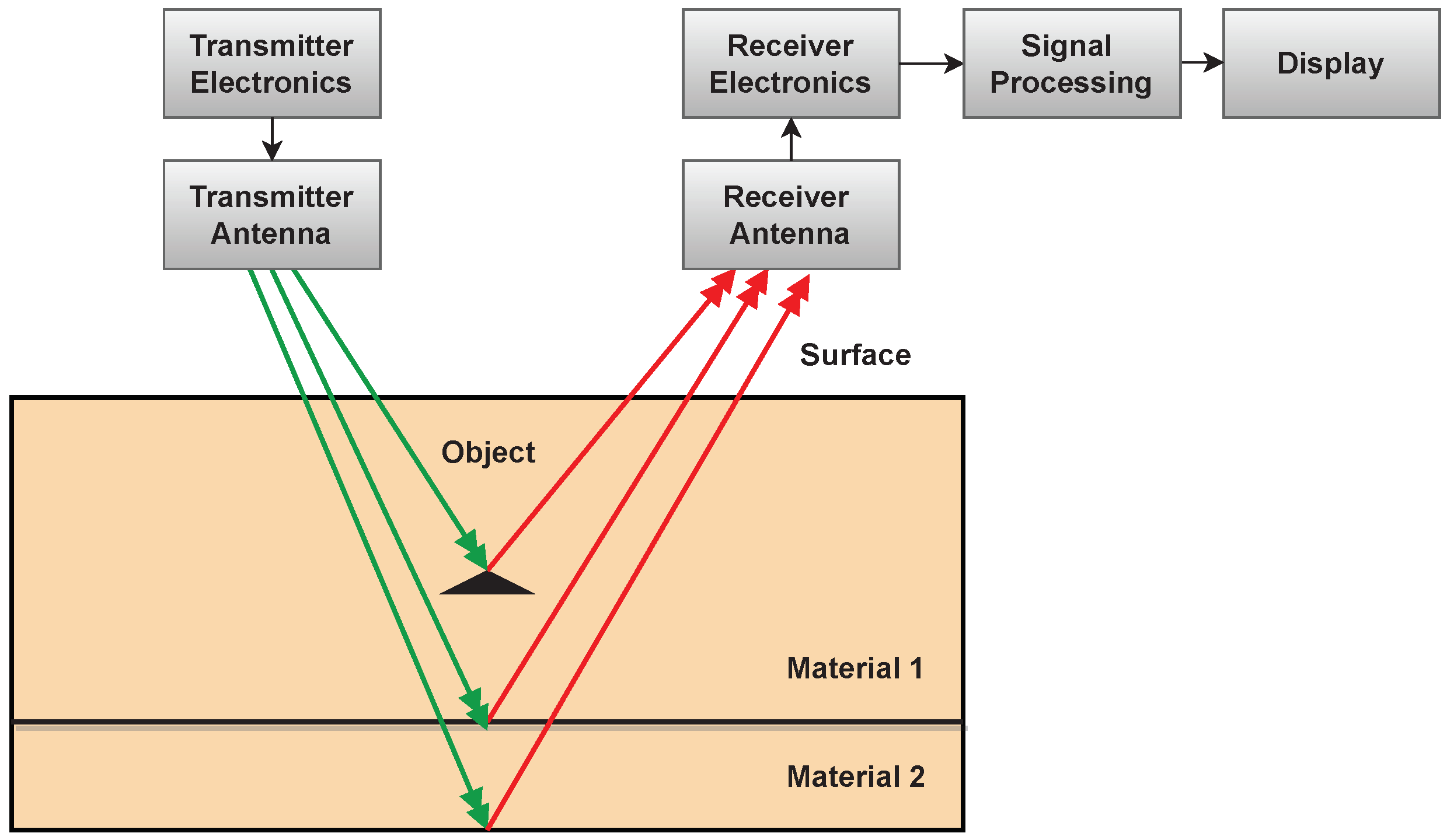
- Electromagnetic and Magnetic Methods [123,124,125]: Either transmitted or reflected electromagnetic waves pass through an element during electromagnetic testing. Changes in the material’s properties are reflected in changing electromagnetic behavior and inclusions (such as steel reinforcement), and voids within a component can be detected. No electrical current flows through the element in these tests since the waves are not electrically coupled. These methods include (1) Eddy Current Testing, (2) Magnetic Flux Leakage, (3) Microwave, (4) Remote Field Testing, (5) Near-Field Testing, (6) Magnetic Particle Inspection, and (7) Ground-Penetrating Radar (GPR).
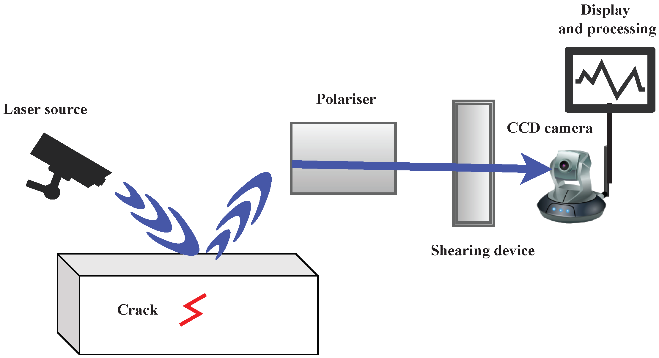
- Optical Methods [126,127,128]: Optical NDT (ONDT) techniques were likely the first methods to be used for NDT, in particular visual testing. ONDT methods offer several advantages, such as fast and contactless measurements. The non-contact nature of the measurements ensures that the object’s state is not altered and does not influence the measurement results. Specific quantities (e.g., color or reflectivity) can almost exclusively be measured optically. ONDT techniques can be categorized into two types, passive and active. Passive ONDT methods use measurement methods like ellipsometry, reflectometry, or simple visual inspection to detect defects. In active ONDT, hidden defects are detected using an excitation force, such as heating or mechanical vibration introduced by transducers. Many parameters can affect optical measurements, including the object’s physical properties, material anisotropy, stresses, and temperature. As such, a laser-excited Lamb wave propagating on carbon fiber-reinforced plastic (CFRP) has different damping and velocity depending on the propagating direction [129]. ONDT methods include (1) Visual Inspection, (2) Fibre Optics, (3) Fibre Bragg Grating, (4) Laser Shearography, (5) Infrared Thermography, (6) Digital Image Correlation, (7) Electric Speckle, (8) Optical Coherence Tomography, (9) Endoscopic and (10) Terahertz technology.
- Radiographic Methods [130,131]: In radiography, ionizing and non-ionizing radiation is utilized to examine the internal structure of objects. The object absorbs some radiation energy depending on its density and structural composition, and energy differentials can be captured using a detector such as a photographic film or digital detector. These methods include (1) X-ray Testing, (2) Gamma Ray Testing, (3) Neutron Radiography, (4) Radiographic Testing, and (5) Neutron Moisture Gauge Testing.
- Electrical and Electrochemical Methods [132,133]: In electrical methods, electricity is applied to an element resulting in a net flow of alternating or direct current throughout the element, while during electrochemical testing, an element’s electrochemical potentials are measured using a reference cell. These methods include (1) Corrosion Current, (2) Electrical Conductivity, (3) Corrosion Half-Cell Potential, (4) Capacitive/Resistive Humidity Sensors, and (5) Alternating Current Field Measurement.
- Chemical and Mass Transport Methods [134,135,136]: During chemical testing, a chemical is directly applied to an element, with the chemical response acting as a guide to determine the element’s chemical and mechanical state. Mass transport testing is performed to determine either a specific or crucial transport factor, such as porosity. Coefficients of these testing types include hydraulic conductivity (D’Arcy permeability), diffusivity, sorptivity (water uptake), and vapor diffusion (drying rate). Chemical and mass transport methods include (1) pH Testing, (2) Staining (Alkali-Silica Reaction), (3) Carbonation Depth, (4) Maturity/Thermometry, (5) Chloride Analysis, (6) Liquid Penetrant, (7) Dye Penetrant, (8) Leak Testing, (9) Permeability, (10) Sorption and (11) Absorption Testing.
- Mechanical Impact Methods [137,138]: In this type of testing, a mechanical impact is imparted on an element generating a static stress field. Typically, the impact goes beyond the elastic behavior of the material, and its mechanical properties are determined, including the point of failure (strength). These methods include (1) Rebound Method, (2) Penetration Resistance, (3) Pullout Testing, and (4) Break-Off Testing.
3.3. Sensor Technologies for NDT Systems
3.3.1. Ultrasonic Technologies
- Ultrasonic Proximity Sensors: An ultrasonic proximity sensor uses a particular type of sonic transducer to transmit and receive sound waves alternately.
- Ultrasonic 2-Point Proximity Switches: This sensor has two switching points and hence has two separate outputs.
- Ultrasonic Retro-reflective Sensors: An ultrasonic retro-reflective sensor works similarly to an ultrasonic proximity sensor, with the difference that it measures the propagation time between the sensor and the reflector.
- Ultrasonic Through Beam Sensors: An ultrasonic through-beam sensor comprises two components: an emitter and a receiver. In the receiver, switching and evaluation outputs are provided.
- Advantages: Ability to characterize material properties; can identify, quantify, and localize internal defects; applicable to various materials and components; allows for single-sided assessment; appropriate for assembling lines; fairly affordable; suitable for in situ inspections owing to portable and compact equipment; can detect discontinuities both on the surface and subsurface; long-range inspection capability; minimal preparation requirements.
- Disadvantage: Trained professionals are required to interpret complex wave features and multi-wave modes; limited computing power and algorithms impose resolution restrictions; advanced methods can have complex system setup and transducer designs; highly responsive to environmental and operational changes; damage identification in the vicinity of the transducer probe can be challenging; requires an accessible surface to transmit ultrasound.
- Blanking Distance (or Dead Band): Sets the distance, starting at the sensor face, to the point where the sensor will start measuring target signals.
- Pulses: Controls how many sound waves are sent in each ultrasonic burst.
- Sensitivity: Controls the amplification level applied to a returning signal from the target.
- Temperature Compensation: A correction factor for changes in air temperature.
- Averaging: Defines the number of target samples (readings) that will be averaged to calculate a distance reading.
- Analog Output: Sets the application’s minimum and maximum sensing range.
- Relay Set Points: Sets the minimum and maximum readings desired from the sensor for control purposes.
- Phased Array Ultrasonic Testing (PAUT): This advanced ultrasonic testing method can be used to inspect welds, assess corrosion, measure thickness, monitor structures, inspect rolling stock (wheels and axles), and perform medical imaging. A phased array ultrasonic scanning unit contains crystals arranged in a pattern to send sound waves in different directions in a material. The technology offers the following advantages: (1) The inspection is fast since no manual sensor movements are required; (2) defect detection is more accurate since a single probe scans all directions simultaneously, reducing additive errors from using multiple angle probes; (3) it provides multiple views of defects using advanced presentation views, such as C-scan view (top view), B-scan view (depth view), S-scan view (sectorial view), and conventional A-scan view (echo pattern). Consequently, the technology is considered a reliable inspection process. An evolution of the PAUT technique is full matrix capture (FMC) which uses the same probes. This method has the advantage of not requiring focusing or steering since the entire area of interest is focused. In addition, it is relatively tolerant of structural noise and misaligned flaws, making it very simple to set up and use. In contrast with conventional PAUT, the recorded data files are huge, resulting in slower acquisition speeds. To improve and automate the data analysis, the capabilities of using machine learning models machine on FMC data were investigated by Siljama et al. [182]. The researchers compared the model performance to the results of a human inspector using real thermal fatigue cracks with similar weld geometries used in training. The results showed a high flaw detection performance using the automated machine learning approach.
- Time of Flight Diffraction Ultrasonic Testing (TOFD): A TOFD system consists of two ultrasonic probes, a “transmitter” and a “receiver” attached to a fixture. There are two types of fixtures: manually operated and robotically operated. This technology detects defects by analyzing the time of wave travel and the diffraction of the wave from crack tips. Hence the name of the test, “Time of Flight Diffraction”. The TOFD technique offers the following advantages: (1) Reliability and reproducibility of inspection; (2) accurate sizing of the depth of the tips; (3) easy storage of the results; (4) quick references and comparisons; (5) monitoring of defect propagation.
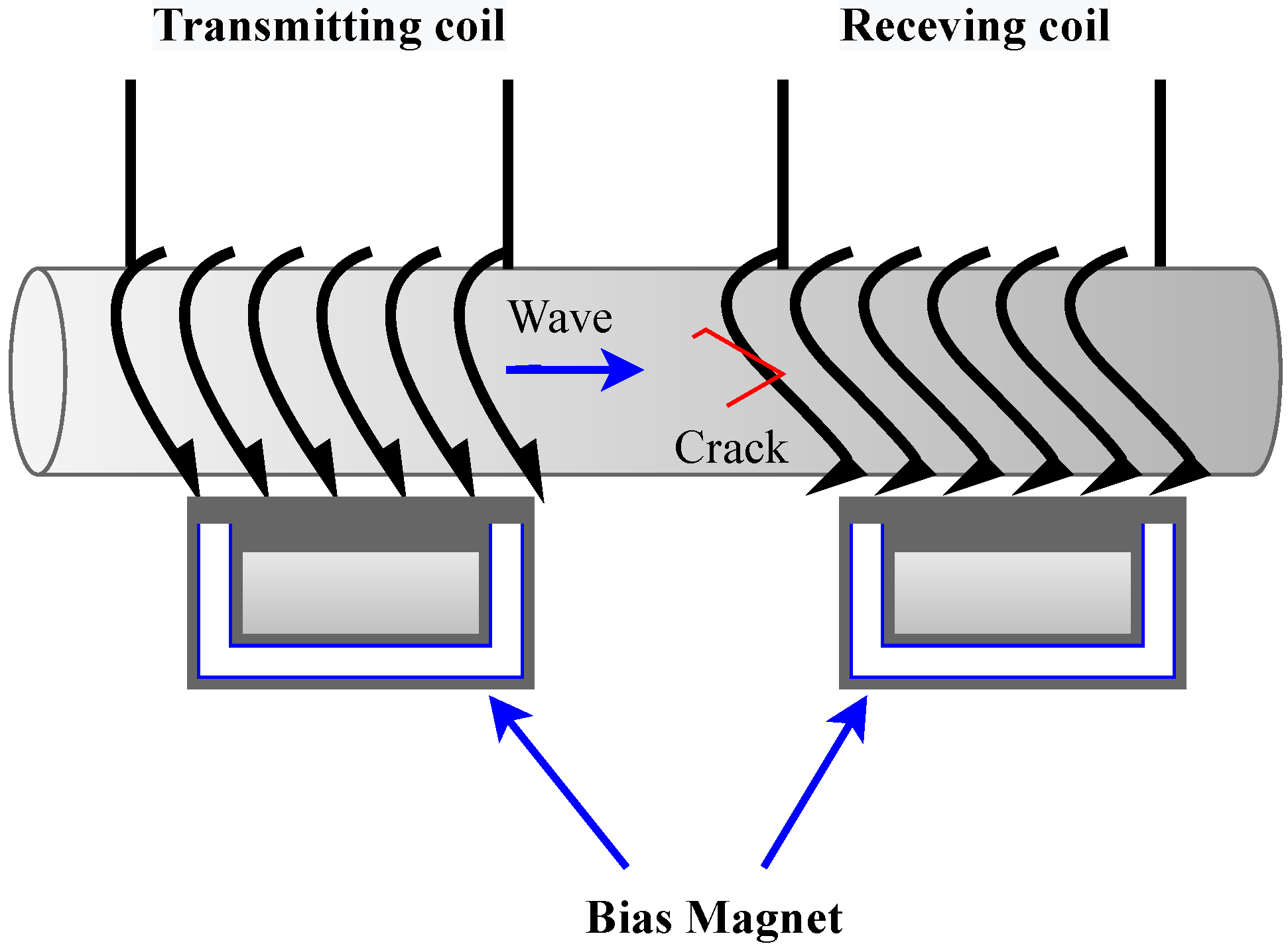
- Long Range Ultrasonic Testing (LRUT): This method, also known as guided wave ultrasonic testing, is a cost-effective and fast technique to inspect long pipelines. Using this technology, the complete length of a pipe can be assessed for internal corrosion, damage, or cracks. In LRUT, multiple probes are positioned around the pipe’s circumference, and waves are transmitted by traveling through the pipe wall. Using low-frequency sound waves will prevent the loss of sound due to scattering. A-symmetrical sound echoes indicate locations of defects, and their size can be determined through the distance amplitude curve (DAC). LRUT has the following significant advantages: (1) It is a fast and flexible testing method; (2) an extended length of pipe can be assessed at once; (3) it can scan insulated and underground pipes without the need for excavation.
- Laser Ultrasonic Testing (LUT): LUT uses lasers to generate and detect ultrasonic pulses for non-contact ultrasonic measurements. Sound pulses are generated by short-pulse, high-energy lasers. Due to the lack of physical contact, this ultrasonic technology can be applied to materials of any temperature. As a result, it is ideal for the in situ assessment of solid metallic and ceramic materials up to their melting point. This technology has the following benefits: (1) Remote and non-contact testing, enabling the inspection of samples at shallow and very high temperatures, for example, during welding with restricted access; (2) small and adjustable footprint; (3) allows the inspection of small and complex geometries; (4) uses high wave frequencies to detect microscopic flaws. Lv et al. [6] developed an automatic non-contact LUT to quantify the depth and width of subsurface defects on metallic components using ML algorithms. The objective of this study was to present and compare three widely used machine learning models in NDE, namely, extreme gradient boosting (XGBboost), adaptive boosting (Adaboost), and support vector machines (SVM), in combination with principal component analysis (PCA) for detecting both the depth and width of subsurface defects. The PCA-XGBoost analysis of laser-ultrasonic signals achieved the highest recognition rate, 98.48%, and was therefore found to be the most effective approach.
3.3.2. Electromagnetic and Magnetic Technologies
- Advantages: Fast; contactless; sensitive to surface defects; detection through several layers and through surface coatings possible; portable; sensitive to small discontinuities; accurate conductivity measurements; can be automated
- Disadvantages: Limited to electrically conductive materials; very susceptible to magnetic permeability changes; unable to detect defects parallel to surface; not suitable for complex geometries or large areas
- Magnetic position sensors: These types can detect magnetic fields and identify an object’s positional data. Sensors include Magnetic switches, Linear sensors, Angle sensors, and 3D magnetic sensors.
- Magnetic speed sensors: These sensors measure the speed (and direction, if required) of rotating targets. Examples are Crank speed sensors, Cam speed sensors, Wheel speed sensors, TLE5549 (new TMR magnetic sensor for autonomous parking), and Transmission speed sensors.
- Magnetic Flux Leakage (MFL): This inspection aims to detect flaws and material degradation in steel components and structures using electromagnetism. In MFL, magnets are used to magnetize a part temporarily, and if flaws are present, the magnetic field created will show distortions, indicating pitting, corrosion, and wall loss on the part. The technology offers the following advantages: (1) A quick and easy way to detect corrosion in ferromagnetic materials; (2) sensitive to pits of corrosion; (3) suitable for finned tube inspections.
- Tangential Eddy Current (TEC): Another magnetic induction-based inspection technique. Tangential ECT differs from conventional ECT in that the coils are oriented tangentially to the surface. The technology offers the following advantages: (1) Weld cap scanning is possible with the probe design; (2) Crack detection and characterization in carbon steel; (3) Multi-element array probes can cover an extensive area in a short period; (4) Surface preparation or coupling is not required.
- Eddy Current Array (ECA): This method represents an evolution of conventional ECT. By using multiplexed arrays of coils arranged in rows, this method is superior to ECT technology (which uses nothing more than one or two coils). The technology offers the following advantages: (1) Maintaining a high resolution while scanning a large area at once; (2) Reduced requirements for complex robotics to move the probe; (3) A more accurate flaw detection due to C-scan imaging; and (4) Complex shape inspection.
- Pulsed Eddy Current Testing (PEC): This inspection is based on the magnetic field penetration through several layers of insulation or coating to induce eddy currents on the surface of a material. Generally, PEC is used to measure the thickness or detect corrosion on ferrous materials that are covered with insulating fireproofing layers or coatings. Applications include corrosion under fireproofing (CUF), corrosion detection under insulation (CUI), and corrosion blisters and scabs. The technology offers the following advantages: (1) During an inspection; there is no need to shut down the equipment; (2) Insulation material is not altered during inspection; (3) No contact is required between the probe and the component under examination; (4) Surface preparation is not necessary; (5) Component thickness is measured.
- Remote-Field Eddy Current Testing (RFEC): This electromagnetic inspection is particularly suitable for examining ferromagnetic tubes from the inside. In order to generate eddy currents within a tube wall, an exciter coil generates a magnetic field on the inside. By appropriate frequency selection, the depth of the skin equals the thickness of the wall; therefore, eddy currents are generated throughout the wall. The technology offers the following advantages: (1) No contact with the test subject is required; (2) Coverage of a large area; (3) It is highly sensitive to variations in wall thickness; (4) Flexible and portable probe.
- Electro-Magnetic Acoustic Transducer (EMAT): An EMAT generates ultrasonic waves into a test object through electromagnetic induction with two interacting magnetic fields. The Lorentz force can be generated similarly to an electric motor by interacting a relatively high-frequency field produced by electrical coils with a low-frequency or static field produced by magnets. This disturbance induces elastic waves in the material’s lattice. The interaction of elastic waves with a magnetic field induces currents in the receiving EMAT coil circuit in a reciprocal process. When magnetostriction is present in ferromagnetic conductors, it produces additional stresses that can enhance the signals much more than can be achieved via Lorentz force alone. They are used in various applications, such as the inspection of in-service piping, the inspection of tubular, and the inspection of vessels. The technology offers the following advantages: (1) Capacity for dry inspections; (2) Imperviousness to surface conditions; (3) Unique wave modes such as shear waves with horizontal polarization.
3.3.3. Shearography Technologies
- Advantages: Non-contact method; suitable for large areas of structures; relatively low sensitivity to environmental variations; ideally suited for honeycomb structures.
- Disadvantages: Possibility of damaging the test specimen, only suitable for specimens with rough surfaces (surface roughness larger than one wavelength of light), requires adequate lightning.
- Laser shearography: This optical surface measurement technique is based on laser-speckle shearing interferometry [217].
- Vacuum shearography: This method is highly effective in diagnosing delamination, core damage, disbonding, and splice joint separations in composite materials [214].
- Thermal pulse shearography: This inspection technique is used for non-visible impact and pressure damage in composite-wrapped pressure vessels [218].
- Vibration shearography: A novel technique recently developed for NASA’s space shuttle’s external tank foam [219].

| NDT Type | Description | Refs |
|---|---|---|
| Dynamic phase-shifting shearography | This paper presented a dynamic phase-shifting shearography system based on a common-path interferometer. The theoretical analysis showed that shearography applications could be more reliable using the proposed system. | [224] |
| Digital shearography | A single-camera digital shearography system was proposed with dual sensitivity to measure minor and extensive shearograms within the same measurement field. Experiments were conducted to evaluate the system’s performance for dynamic imaging of an object with defects. | [225] |
| Acoustic shearography | This paper used acoustic shearography imaging to detect defects in carbon fiber composite materials. The results of acoustic shearography provided sufficient defect imaging with significantly reduced imaging time compared to X-ray computed tomography. | [226] |
| FEM-assisted shearography with spatially modulated heating | Shearography was advanced towards a quantitative inspection tool for thick composites utilizing the finite element method (FEM). According to the results, the proposed spatially modulated heating (SMH) approach improved deep defect detection in thick composites by 2 to 3 times compared to global heating (GH). | [227] |
| 2D shearography | A two-dimensional (2D) shearography with source displacement was proposed for measuring object contours. In the experimental work, spherical and hyperbolic paraboloid surfaces and objects with different types of surfaces were tested, and contours were successfully measured. | [228] |
| Dual shearing direction shearography | Based on a spatial light modulator (SLM), this study proposed a dual shearing shearography system. Its simple structure, relative light efficiency, and good phase map quality make this system more advantageous than spatial phase shift shearography. | [229] |
| Spatial phase-shift shearography | Dual-direction sheared spatial phase-shift digital shearography (DDS-SPS-DS) were proposed to measure strain/displacement derivatives simultaneously. Two Michelson Interferometers were used as shearing devices to create two shearograms, one in the x-shearing direction and one in the y-shearing direction. A single CCD camera was used for the recording. | [230] |
| Pixelated carrier phase-shifting shearography | The aim of this work was to develop a pixelated carrier phase-shifting shearography based on a spatial-temporal low-pass filtering algorithm. By simultaneously low-pass filtering the phase maps in the spatial and temporal domains using the algorithm in the complex domain, the phase maps showed better phase quality. | [231] |
3.3.4. Infrared Technologies
- Advantages: Affordable and fast operation; real-time implementation; compatible with a variety of materials; damage visualization; single-sided inspection; safe procedure (non-ionizing radiation).
- Disadvantages: Delicate equipment, unsuitable for field testing; the precision is affected depending on the specimen geometries and complexities; restrictions are imposed due to the expense and accessibility of excitation sources in the field; computing power and algorithms determine the processing time for data; identifying cracks will require higher automation from footage; offshore structures may have difficulty implementing the application.
- Wavelengths and electromagnetic spectrum: Radiation is characterized by its wavelength and frequency. The electromagnetic spectrum covers waves with frequencies ranging from below 1 Hz to above Hz. Infrared radiation covers a range from roughly 300 GHz to 400 THz (1 mm–0.78 m) and is invisible to the human eye. Several sub-divisions exist in the infrared spectrum, with each having its own characteristics:
- –
- NIR (near infrared): These are wavelengths in the infrared spectrum close to the visible spectrum, between 0.78 m and 2.5 m.
- –
- SWIR (short wave infrared): The spectrum from 1 m to 2.7 m.
- –
- MWIR (medium wave infrared): The spectrum from 3 m to 5 m.
- –
- LWIR (long wave infrared): The spectrum from 7 m to 14 m.
- –
- FIR (far infrared): The spectrum from 14 m to 1000 m.
- Detector: An infrared detector can detect radiation from the infrared spectrum. Current detectors can be classified into two types:
- –
- Cooled: These detectors are maintained at shallow temperatures using cryogenic cooling. This system lowers the sensor temperature to cryogenic temperatures, which reduces heat-induced noise to a level lower than the scene’s signal.
- –
- Uncooled or microbolometers: These detectors do not need a cooling system. Here, the temperature of the microbolometer changes when temperature differences occur in a scene.
- Indicator of detector sensitivity: Thermal sensitivity is measured by NETD (noise-equivalent temperature difference). This is the smallest temperature difference that a camera is capable of detecting. The temperature is expressed in milliKelvin (mK) or degrees Celsius (°C). NETD determines how well a camera can detect thermal contrast the lower the number, the better the sensitivity. In terms of contrast, NETDs are analogous to visible light detectors.
- Resolution and field of view (FOV): A camera’s FOV indicates the range/angle of light that can be captured. The FOV of an image must be considered in conjunction with its resolution (the number of pixels).
- Analog or digital: Analogue-to-digital converters (ADCs) convert analog signals to digital (binary) signals. Digital-to-analog converters (DACs) convert digital signals into analog signals.
- Planck’s Radiation Law: Radiation is emitted by every object at a temperature T not equal to 0 Kelvin.
- Stephan Boltzmann Law: The total energy emitted by a black body at all wavelengths is proportional to its absolute temperature.
- Wein’s Displacement Law: Different objects emit different wavelength spectra at different temperatures.
3.3.5. Radiographic Technologies
- Advantages: Detection of surface and internal flaws; ability to inspect hidden areas; minimal preparation; few material limitations; high resolution
- Disadvantages: Health and environmental impact of radiation; requirement of safety protective equipment; high degree of skills and experience; slow process; only qualitative but not quantitative results; high voltage requirements; expensive; ineffective for planar and surface defects.
- Analyzing variations in structures;
- Analyzing material thicknesses and tracking changes;
- Detection of cracks and voids;
- Tracking minute surface changes;
- Assessing porosity.
- Film radiography: Although this technology has been around for over 100 years, it is still highly regarded and widely used. Film radiography has a high spatial resolution and provides high-quality results. However, the film is produced with potentially harmful chemicals, and the development is time intensive.
- Computed radiography (CR): In CR, a phosphor imaging plate is used instead of a film. This requires less exposure time, and results are obtained quickly and without chemical processing. In addition, phosphor plates have an excellent dynamic range and are more sensitive than films. The image captured on a phosphor plate is converted into a digital signal which can be viewed on a computer monitor and stored digitally for later review and archive.
- Fluoroscopy: Fluoroscopy enables continuous and real-time examination of large structures, making it a cost-effective and practical solution. As a result, this method is not as sensitive as others and provides images of lower resolution.
- Digital detector array (DDA) radiography: Furthermore, this method, known as direct radiography, is similar to computed radiography. In digital imaging, an electronic flat panel detector captures and displays an image directly on a computer screen instead of using a film scanner. It produces higher-quality images and has shorter exposure times than CR, but it is more expensive and less portable than CR or film.
3.4. Ground Penetrating Radar
- Advantages: Non-invasive, non-destructive, and safe to use in public areas; fast data collection; suitable for large-area scanning; accurate depth, location, and dimension assessment of small and large objects; scanning at different depths and resolutions is possible with multiple frequencies; interpreting data in real-time or processing it off-site is possible; subsurface scanning is faster, safer, and more affordable than other methods.
- Disadvantages: Signal scattering limits performance in heterogeneous conditions (e.g., rocky soils); interpretation of radargrams is generally non-intuitive to the novice; designing, conducting, and interpreting GPR surveys requires considerable expertise; for extensive field surveys, relatively high energy consumption can be problematic.
3.5. Laser Scanning Photogrammetry
- Advantages: Rapid and thorough technology; high accuracy; non-contact testing; cost-effective; safe.
- Disadvantages: Accuracy reduction from light interferences of ambient sources; high initial investment; incapable of measuring surfaces beyond the range of the scanner.
3.6. Other NDT Approaches
- Dynamometer testing: This technique was developed to identify potential slipping in the high-speed shaft tapered roller bearings in drive train systems [285];
- Sound-based monitoring using audio speakers: This method was used to ensonify the internal cavities of WT blades and arrays of external microphones detecting patterns in airborne sound waves [286];
- Short-range Doppler radar: This technique was recently tested for on-site SHM of wind turbine blades [287];
- Multi-sensor apparatuses: This approach uses multiple types of sensors, such as optical, acoustic, and vibrational sensors, to detect bird strikes and bad strikes [288].
4. SHM Systems
- In SHM, existing civil structures are characterized to identify and detect structural defects [300].
- SHM involves continuously interrogating sensors installed within a structure to extract characteristics indicative of the structure’s current state [301].
- In SHM, different parts of the structure are continuously diagnosed and assembled as a whole so that the entire structure can be diagnosed continuously [302].
4.1. Benefits of SHM Technologies
- Active safety monitoring and control: Alert systems can inform asset managers if prescribed limits are exceeded, such as when abnormalities in load or responses occur, ensuring human and structure safety.
- Environmental monitoring: Site-specific environmental conditions such as wind and temperature can be evaluated.
- Improved structure assessment: The reliability and accuracy of structural assessments can be improved based on up-to-date structural response data.
- Optimization of maintenance: An optimal inspection, maintenance, and repair schedule can be determined on an “as needed” basis when indicated by monitoring data, resulting in cost reductions.
- Real-time safety assessments can be performed during normal operations or immediately following extreme events.
- Assumptions and parameters related to the structure design can be validated, resulting in improvements in future specifications and guidelines.
- Future performance can be predicted based on past and current monitoring data.
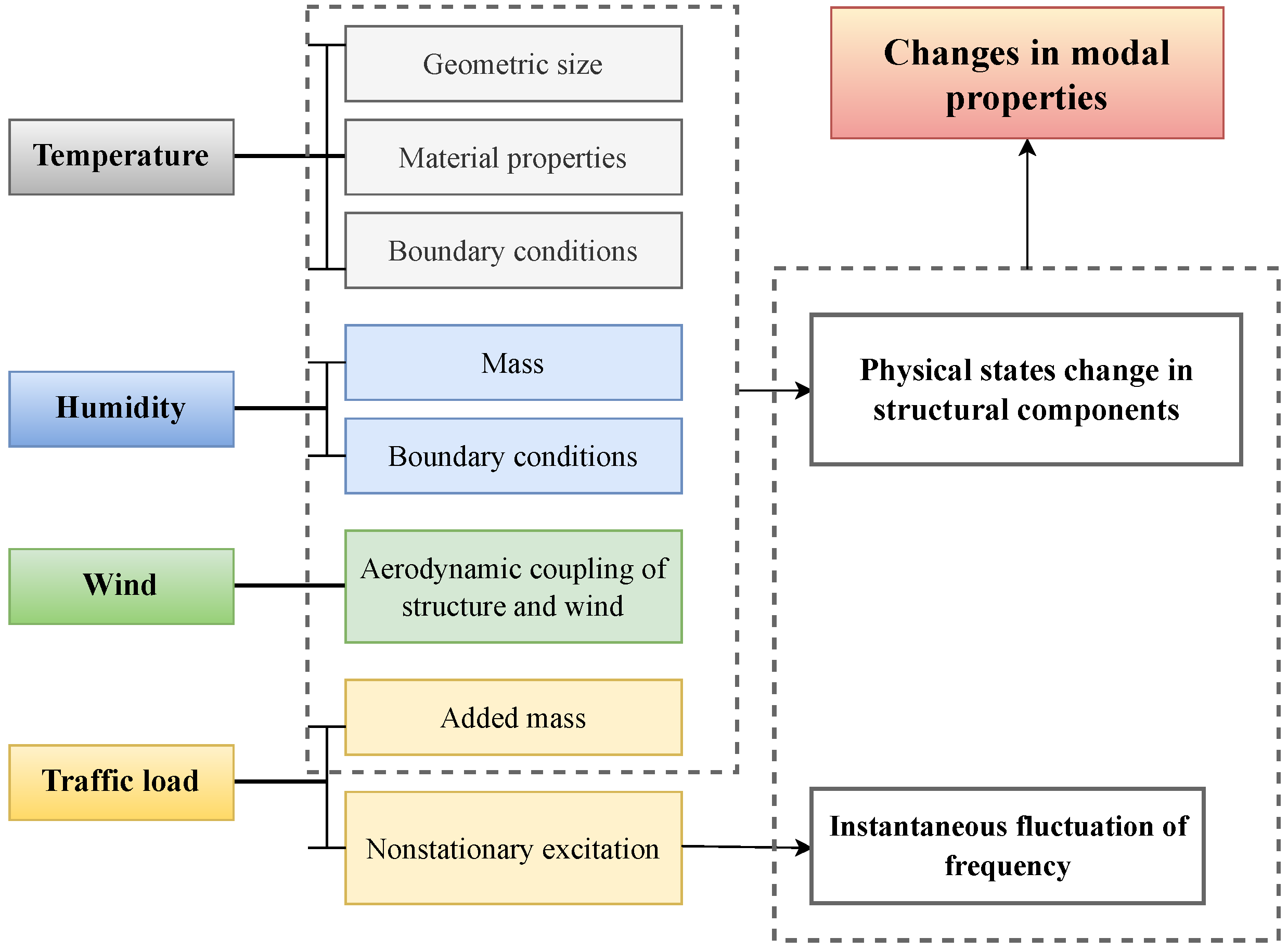
4.2. Environmental and Operational Conditions (EOCs) Effects
- Input–output methods include multiple polynomial regression (MPR), multiple linear regression (MLR), and support vector regression (SVR).
- Output–only methods include principal component analysis (PCA), cointegration analysis (CA), auto-associative neural network (AANN), and Mahalanobis squared distance (MSD).
4.3. SHM Strategies
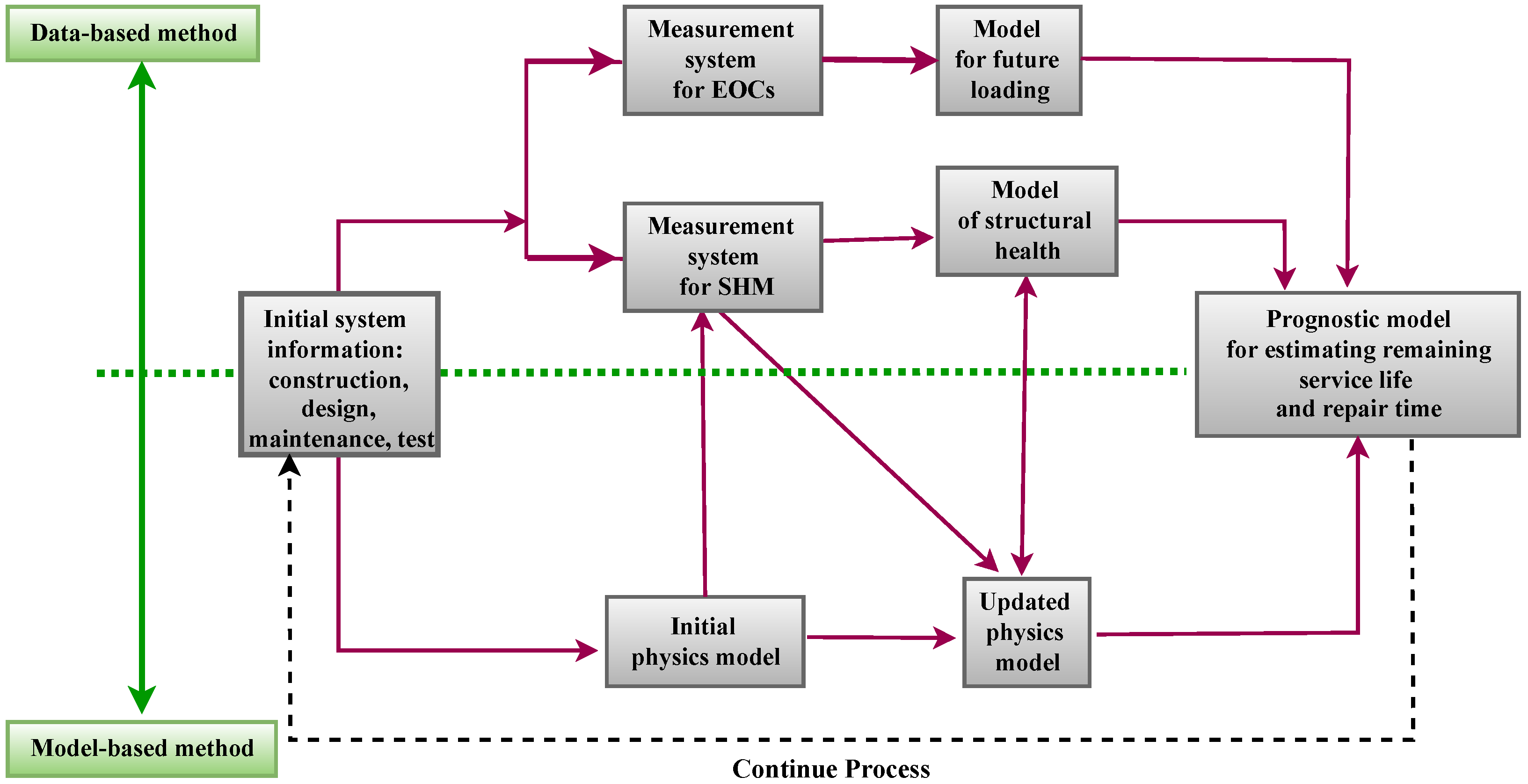
4.3.1. Model-Based SHM Systems
- Advantages: (1) Predictions can be made about the impact of variations in loading and usage, (2) potential consequences of future damage can be evaluated, (3) insights and recommendations for further inspections and measurements can be made, (4) if causal links can be established between measurements and possible causes, data interpretation becomes simpler, (5) rehabilitation and repair planning can be supported, (6) can assist in making better maintenance decisions.
- Disadvantages: (1) Modeling is time-consuming and costly, (2) modeling errors may result in false identifications and predictions, (3) managing a large number of candidate models can be difficult, (4) several interpretation-measurement cycles may be needed to identify the correct model, and (5) combinatorial challenges may arise with complex structures.
4.3.2. Data-Based SHM Systems
- Advantages: (1) No system model required, (2) a wide range of signal analysis options, (3) no damage studies required, (4) damage accumulation can be tracked by incremental training, and (5) capable of detecting situations requiring model-based interpretation over long periods.
- Disadvantages: (1) Potential misinterpretation of signals, (2) indirect guidance for structural management activities, (3) insufficient capabilities for rehabilitation decisions, and (4) unsuitable for justifying replacement avoidance.
4.4. Sensing Systems for SHM
- Monitoring objectives;
- Sensor types, numbers, and placements;
- Sensor measurement characteristics;
- Sensitivity, bandwidth, and dynamic range;
- Continuous or periodic sampling intervals;
- System installation constraints;
- Power demands;
- Data transmission;
- Telemetry, data acquisition, and storage system;
- Excitation source (for active sensing);
- Memory and processor requirements;
- Resilience of the system in the case of malfunctions;
- Data Analytics.
- Increasing the robustness of the intended measurements;
- Enhancing the system’s robustness and reliability;
- Reducing uncertainty in the monitoring results in systems.
4.4.1. Sensor Technologies for SHM
- Active or passive sensing [299]: Active sensors need an excitation or power signal from an external source. On the other hand, passive sensors, do not require any external power source and generate output directly.
- Detection substance [348]: Different substances such as electric, biological, chemical, and radioactive can be detected.
- Conversion method [349]: Conversion types include photoelectricity, thermoelectricity, electrochemistry, electromagnetics, and thermoplastics.
- Analog and digital [349]: Analog sensors measure physical quantities, including voltage or resistance, while digital sensors produce discrete output values (0 and 1’s).
- Application type: For instance, Sehrawat and Gill [350] categorized sensors suitable to the Internet of Things (IoT), including proximity, temperature, humidity, chemical, position, motion, and pressure sensors.
- Other classifications include sensor specifications, material type used, cost, and power source.
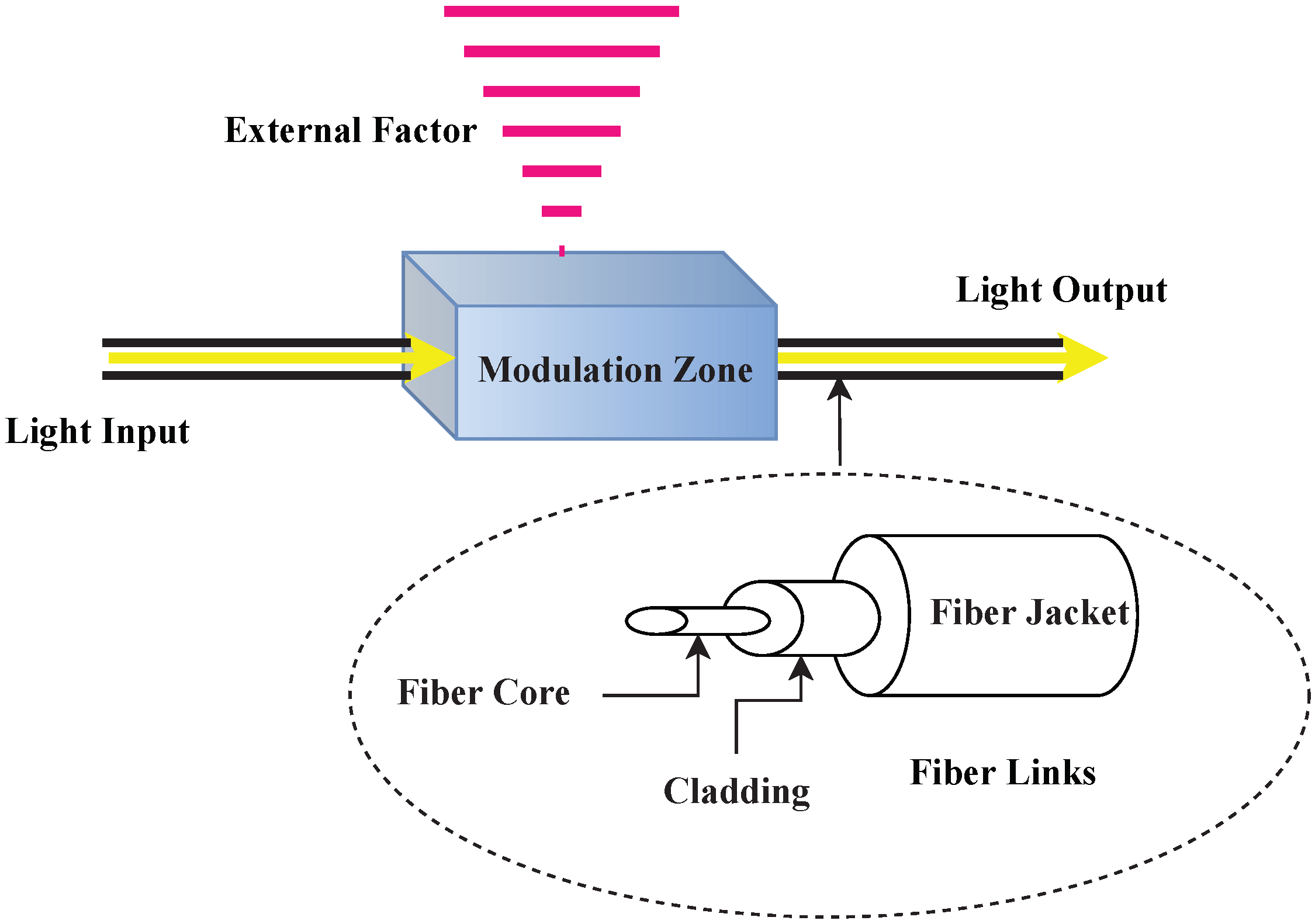
4.4.2. Fiber Optic Sensors (FOSs)
- FOSs have low signal transmission loss enabling remote monitoring and transmission over long distances.
- They are insensitive to electromagnetic interference.
- They offer a great variety of measurable parameters.
- A single optical fiber can have distributed or multiplexed topologies, allowing it to capture full distribution measurements.
- They are corrosion-resistant and have excellent long-term stability and continuous monitoring capability.
- Sensors and cabling are small and lightweight.
- FOS can be permanently integrated into structures.
- They can withstand severe environments such as extreme temperatures, radiation, and vacuum.
- SOFO sensors [353]: Surveillance d’Ouvrages par Fibres Optiques (SOFO) interferometric sensors (dynamic and static systems) are long base sensors, measuring from 200 mm to 10 m. This system uses low-coherence interferometry to measure the lengths of a pair of single-mode fibers, a measurement fiber, and a reference fiber installed on the monitored structure. To capture the structure’s deformations, the measurement fiber is pre-tensioned and mechanically attached at two anchorage points, while the reference fiber is placed loosely in the same tube. Independent of the measurement base, the sensors have excellent long-term stability and precision of 2 m. Since displacement information is encoded in the coherence of light rather than the intensity of the light, changes in the fiber transmission properties do not affect precision. Since the length difference measurements between the fibers are absolute, the reading unit and the sensors cannot be permanently connected.
- Fabry–Pérot interferometric sensors [354]: Fabry–Pérot sensors are point sensors that utilize optical cavities formed by two parallel reflecting surfaces to measure physical changes. Measurement is achieved by recording the Fabry–Pérot cavity’s length using white light interferometry. The sensors can be active or passive. Extrinsic Fabry–Pérot interferometers (EFPIs) are capillary glass tubes containing two partially mirrored optical fibers adjacent to each other with a remaining air cavity of a few micrometers between them. Two mirrors produce a back-reflected interference signal when light is launched into one of the fibers. Coherent or low-coherence techniques can demodulate this interference and reconstruct the changes in the fiber spacing. Capillary tubes are generally attached at their extremities with a space of 10 mm between them. Changes in the cavity can be correlated with strain variations between the two attachment points. Fabry–Pérot sensors are accurate, simple to use, versatile, and immune to environmental noise. They are typically used to measure strain, temperature, pressure, and displacements.
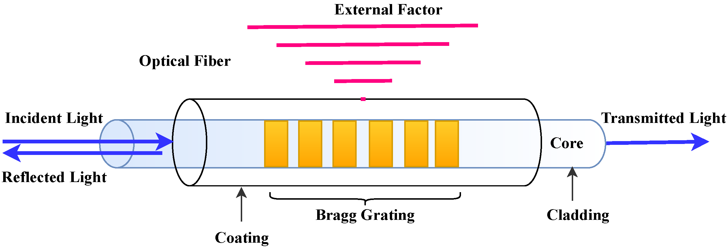
- Fiber Bragg grating (FBG) sensors [355]: FBG sensors are quasi-distributed (multiplexed) sensors that work on the principle of Fresnel reflection, where light traveling between media of different refractive indices can reflect and refract at the interface. A Bragg grating is a periodic alteration in the refractive index of the fiber core caused by the exposure of the fiber to intense ultraviolet light of 244 to 248 nanometers. A typical grating length is about ten millimeters. A grating can reflect light at wavelengths related to the grating period, while other wavelengths will be unaffected. Temperature and strain affect the grating period (length), so the spectrum of reflected light can be used to measure both parameters. For SHM of civil infrastructure, FBG sensors have been used to monitor tall structures, tunnel construction monitoring, and water pipe integrity monitoring. Figure 13 shows an overview of an FBG sensor. An application of the Bragg equation to light traveling along a Bragg grating core is given by:where : Bragg’s wavelength; : effective refraction index of the fiber core; P: Period of index modulation.Since the forward and backward propagating modes are coupled, the grating reflects a portion of the illuminated light and transmits the rest. Temperature and strain affect both and P, which is why the Bragg wavelength is sensitive to both factors. One of the most significant features of an FBG sensor is its capability to self-reference. Since the measurement values are encoded into wavelengths, which are absolute parameters, no calibration or reinitialization is required. FBG sensors have advantages over conventional sensors because they have gratings that can be multiplexed and positioned at different locations in the fiber, reflecting different wavelengths. Accuracy in the order of 1 and 0.1 °C can be achievable using the best demodulators.
- Distributed Brillouin and Raman scattering sensors [356]: In optical fibers, Brillouin and Raman’s scatterings result from the interaction of photons with localized material characteristics such as strain, temperature, and density. Due to different dynamic inhomogeneities in the silica fibers, Brillouin and Raman scattering effects have different spectral characteristics. Brillouin scattering operates backward, whereas Raman scattering operates forwards and backward. Emitting intense light at a known wavelength into a fiber causes minimal light to scatter from every location along the fiber. In addition to the original wavelength (i.e., the Rayleigh component), scattered light components are present with wavelengths higher and lower than the original signal (i.e., Raman and Brillouin components). These shifted wavelength components provide information on the local properties of the fiber, such as its strain and temperature. With a single unit, it is possible to measure thousands of points along the length of these fiber optic sensors. Raman scattering systems are typically accurate to ±0.1 °C and possess a spatial resolution of 1 m for measurement ranges up to 8 km. The best Brillouin scattering systems have a strain accuracy of ±20 , a temperature accuracy of ±0.1 °C, and a measurement range of 30 km at a spatial resolution of 1 m.
- Multicore fiber sensors [357]: Multicore optical fibers are waveguides containing several cores. The cores are embedded in a common cladding and are sufficiently spaced to avoid the overlap of modes propagating. Multiple sensors can be accommodated in the same fiber cross-section owing to the independently propagating modes. Fan-outs or graded index lenses are typically used for coupling the different cores. Strain, temperature, vibration, and acoustic waves can be measured with these sensors. By interfering with different propagating lightwaves or wiring FBGs into the different cores, multicore FBG sensors can also be used to measure the curvature of different axes in the fiber cross-section. The cores can be accurately measured since they are located at various locations relative to the neutral bending axes. Inherent axial strain and temperature compensation also allow the accurate measurement of the local curvature.
- Microstructured optical fiber sensors [358]: Optical fiber communication systems and sensors have tremendous potential due to the recent invention of microstructured optical fibers. The cross-sectional geometry of these fibers is complex, including holes for both air and silica. The propagation lightwaves are confined either through a photonic bandgap effect (photonic crystal fibers) or an effective index contrast as in conventional optical fibers with air holes reducing the cladding index of refraction (holey fibers). Sensors applied to these fibers benefit from their complex geometry, providing new sensing opportunities and enhanced response characteristics. This fiber offers the following main advantages for sensing applications: (I) Since the fundamental mode propagates through less silica, the sensors have a near-zero temperature sensitivity; (II) single-mode fibers can be used across a wide wavelength range, allowing multiplexing of sensors with significantly different wavelengths; (IV) chemical sensing applications can be achieved by inserting gas into the air holes, allowing the propagating mode to interact with the gas over an extended surface area; and (V) by arranging the air holes, polarization maintaining (PM) fibers can be fabricated without inducing residual thermal stresses, which improves the stability of the birefringence when the temperature changes.
- Polymer optical fiber sensors [359]: An optical fiber made of polymer is known as a polymer optical fiber (POF). In the design of POFs, various optical polymers are used, including polymethylmethacrylate (PMMA), amorphous fluorinated polymer (CYTOP), polystyrene (PS), and polycarbonate (PC). POFs have a high elastic strain limit, a high fracture toughness, a high degree of flexibility in bending, a higher degree of sensitivity to strain than silica, and a negative thermooptic coefficient. Biocompatibility is another advantage of polymeric materials. A significant obstacle to using POFs as sensors is fabricating them. Generally, POF sensors are based on multimode POFs because of fabrication difficulties. Since multimode POFs are less expensive, they are also easier to connect, but their diameter is greater than that of single-mode POFs. Viscoelastic properties and extreme humidity sensitivity are also characteristics of POFs. A POF sensor may operate at a lower wavelength than an equivalent silica fiber sensor because polymers are highly attenuating in the near-infrared region. Some of the same measurement principles as silica optical fiber sensors are used to demonstrate multimode POF sensors, including intensity losses, backscattering, and time-of-flight measurements. Recently, new capabilities for POF sensors have been developed, including single-mode solid POFs and single-mode microstructured POFs. As a result of the emergence of these optical fibers, high-precision, large-deformation optical fiber sensing has become possible.
- Rayleigh scattering distributed sensors [352]: Distributed optical fibers based on Rayleigh scatter use backscattered light signals from naturally occurring impurities (scatters) in standard optical fibers to achieve sensing without introducing additional markers. This allows for sensors previously distributed over long distances to be replaced with a standard optical fiber, providing distributed measurements over large distances without needing expensive individual sensors. Rayleigh backscattering can be used to measure strain and temperature along the length of the optical fiber. The advantages of using Rayleigh scattering are high measurement rates, high spatial resolution, long-range, and higher efficiency, leading to higher signal-to-noise ratios.
4.4.3. Accelerometers
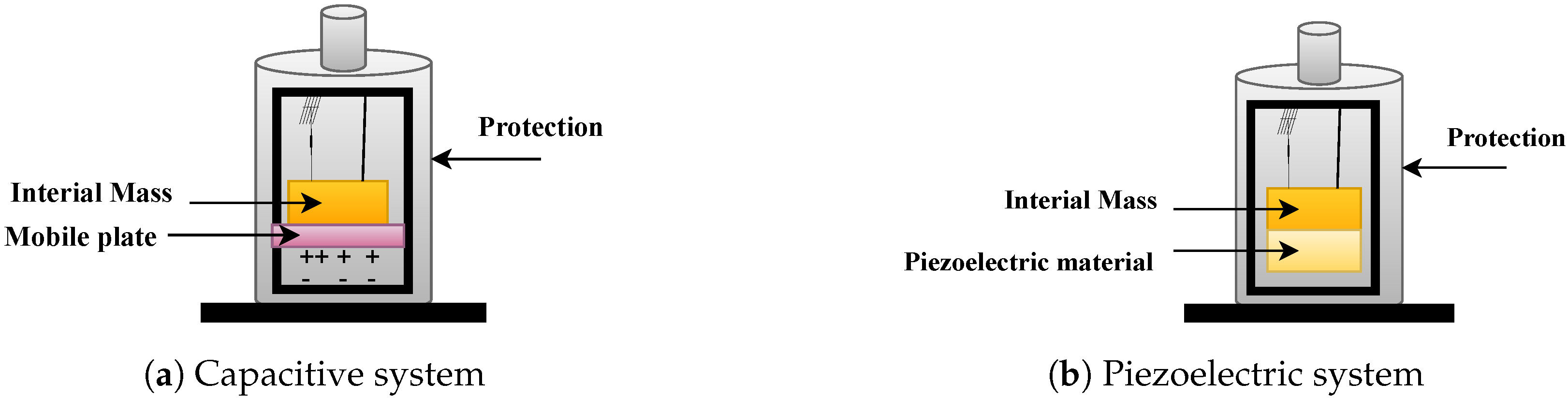
- Piezoelectric: Piezoelectric accelerometers are the most widely used accelerometers in civil and aerospace applications. They typically measure acceleration in one of three modes: shear, flexural, or compression. Piezoelectric materials generate electrical charges in response to net forces acting on them. These materials can be classified as ceramic, polymer, and composite. Due to their electrical-mechanical transformation, piezoelectric materials act as both actuators and sensors at the same time. Since they contain no moving parts, they are long-lasting, can be used across a wide frequency range, exhibit good linearity across a wide dynamic range, and are robust and adaptable to various environments. Due to their minimum frequency requirements, these sensors are not capable of measuring static accelerations, unlike capacitive or piezoresistive accelerometers. In recent years, piezoelectric sensors have been incorporated into several SHM systems of civil engineering structures to measure acceleration, electrical impedance, elastic waves, and acoustic emission. The following lists some examples of SHM-related research and applications:
- –
- A piezoelectric oscillator sensor was developed in [365];
- –
- Impedance measurements were used for damage detection in [366];
- –
- Piezoelectric sensors were used for reference-free crack detection in [367];
- –
- Impedance-based self-diagnosis was investigated for piezoelectric sensors in [368];
- –
- A smart dual PZT transducer for damage detection was developed in [369];
- –
- A wireless sensor network SHM system based on piezoelectric sensors was investigated in [370];
- –
- A low-cost multifunctional wireless sensor node was developed using piezoelectric sensors in [371].
The development of nanoscaled piezoelectric transducers has attracted increased interest due to their ultra-compactness and precision control. Future research on these sensor systems is proposed to focus on long-term ruggedness, miniaturization for increased flexibility, high-temperature applications, and high-strain and high-radiation conditions for permanently installed and embedded sensors. - Force balance: These accelerometers employ active feedback control systems to control the position of a proof mass. Feedback is used to calculate the system’s acceleration keeping the mass stationary. During acceleration of the sensor housing, the proof mass stays stationary relative to the inertial frame of reference. Consequently, the proof mass moves away from its nominal position inside the sensor housing. An error signal is produced in the control system when a displacement sensor (often capacitive) detects this relative motion. Current flows through the force-generating element, balancing the force caused by acceleration. Based on the known proof of mass and system properties, acceleration can be calculated based on the current and force applied. Force balance accelerometers are often used for civil structure monitoring due to their excellent resolution at low frequencies, thermal insensitivity, and relatively nonlinear nature. There are, however, disadvantages of these types of sensors, including an expensive control mechanism and a limited bandwidth compared to other accelerometers. In [372], a force-balance-based accelerometer system was developed for measuring aerodynamic forces at impulse facilities using typical flight configurations. As part of the Indian Institute of Science’s hypersonic shock tunnel (HST2), Saravanan et al. [373] developed and tested a new three-component accelerometer force balance.
- Capacitive: A capacitive accelerometer determines acceleration by measuring the displacement of a proof mass relative to the sensor’s housing. Because the motion of the proof mass is relatively small in a capacitive accelerometer (less than 20 m), it is typically suspended between two plates. Two capacitors measure small drifts and differentials between the mass and the top and bottom plates. Compared to piezoresistive accelerometers, capacitive accelerometers offer superior stability, sensitivity, and resolution, which makes them ideal for monitoring large structures. In contrast to piezo-electric accelerometers, they are somewhat sensitive to temperature and humidity fluctuations. Büsching et al. [374] provide a comprehensive review for the interested reader.
- MEMS: The technology of microscopic devices, particularly those with moving parts, is known as microelectromechanical systems (MEMS), also called microelectromechanical systems (or microelectronics and microelectromechanical systems). Micromechanics and microsystems are related technologies. MEMS devices generally range in size from 20 m to 1 mm (i.e., 0.02 to 1.0 mm), and components range between 1 and 100 m (i.e., 0.001 to 0.1 mm). Arrays of components (such as digital micromirror devices) can reach 1000 mm2. MEMS measure the linear acceleration of objects to which they are attached. The size and affordability of these devices allow them to be embedded in a wide range of hand-held electronic devices (such as smartphones, tablets, and video game controllers). Capacitive and ohmic switches are the two basic types of MEMS switches. MEMS switches with capacitive characteristics have moving plates or sensing elements that change the capacitance. Electrostatically controlled cantilevers control ohmic switches. As the cantilevers deform over time, ohmic MEMS switches can fail from metal fatigue of the actuator (cantilever) and contact wear. Whenever linear motion is required without a fixed reference, such as movement, shock, or vibration, MEMS accelerometers can be used. Lynch et al. [375] presented a detailed discussion of a high-performance, piezoresistive MEMS accelerometer with a planar structure. The performance of representative MEMS devices in SHM applications was presented by Parisi et al. [376], providing insight into the opportunities and capabilities of these devices.
- Piezoresistance: Piezoresistive accelerometers similarly measure stress to strain gauges. A force is applied to a piezoresistive material, and the change in resistance is measured after it is deformed. When pressure is applied to a piezoresistance accelerometer, its resistance increases. As a result of their high bandwidth, piezoresistive accelerometers are ideal for measuring high frequencies in a short period. Their low sensitivity makes them less useful for vibration testing. Interested readers can find a comprehensive review in [377].
4.4.4. Electrochemical Sensors
4.4.5. Magnetostrictive Sensors
4.4.6. Vibrating Wire Strain Gauge
4.4.7. Linear Variable Differential Transducers
4.4.8. Load Cell
4.4.9. Foil Strain Gauge
4.4.10. Tiltmeters
- Monitoring of vertical rotation, deflection, and deformation in retaining walls.
- Monitoring differential settlements on railway lines.
- Assessing the stability of structures in landslide areas.
- Monitoring tunnel movement and convergence.
- Assessing the performance of bridges and struts.
- Inspecting critical structures and utilities affected by excavation/tunneling operations.
- Inspection of dams, piers, and piles for inclination and rotation.
- Monitoring volcanoes for structural changes or deformations.
4.4.11. Laser Doppler Vibrometer
4.4.12. Acoustic Emission Sensor
4.4.13. Temperature Sensors
- Contact temperature sensors: For these sensors, the object being sensed must be in physical contact with the sensor, and temperature changes are monitored via conduction. They can be used on solids, liquids, and gases for various temperatures.
- Non-contact temperature sensors: Sensors of this type monitor temperature changes via convection and radiation. Radiation detectors can detect liquids and gases that emit radiant energy in convection currents or infrared radiation transmitted from objects (the sun).
- Resistive temperature sensors: These types of sensors work on the principle that resistance changes with temperature. Most resistive temperature sensors are either metallic sensors or thermistors. Metallic sensors consist of platinum wires wrapped around a mandrel and are covered with protective coatings or enclosed in protective housings. Platinum resistance changes linearly with temperature. Hence, Wheatstone bridge circuits can be assessed by installing one of these sensors in one circuit arm. A highly nonlinear relationship exists between a thermistor and resistance temperature. To overcome this challenge, matching pairs of thermistors are used to offset their nonlinearities. In general, thermistors are more accurate than metallic temperature sensors, but their operation range is smaller. Ceramic semiconductors can also be used as thermometers due to their change in resistance. It is noted that there are fundamental limitations to all resistive sensors. Even though the current used to operate these sensors is very small, it creates heat, leading to inaccurate temperature readings.
- Vibrating wire temperature sensors: The operation of vibrating wire temperature sensors is similar to that of VW strain gauges. In A VW temperature sensor, changes in the temperature affect the frequency at which the wire vibrates or resonates. The sensor produces a voltage proportional to the temperature reading or displays the temperature in temperature units. Since the VW temperature sensor is enclosed in a cylinder, it cannot physically contact the testing material. Therefore, no special precautions are necessary for strain effects on sensor readings.
4.4.14. Next-Generation Sensing Techniques
- Unmanned Aerial Vehicles (UAVs): Inaccessible surfaces or the requirement to install a large number of sensors limit the affordability of traditional contact-based sensors. Recent advances in non-contact measurement technology were made possible with UAVs, namely, drones. UAVs are aircraft without pilots, crews, or passengers. Rapid developments in control theory, computing capabilities, robotics, communications, and automation technologies provide the platform for the wide variety of applications of UAV technology in SHM systems. UAVs are now equipped with lightweight cameras to take pictures and estimate the structure’s global and local health. Most UAVs are composed of a navigation system with visual servoing, a global positioning system (GPS), and a vision system typically consisting of an out-of-the-box camera (e.g., an infrared camera, optical sensor, or laser detection and ranging (LADAR)). A navigator on the ground can control the aircraft remotely by controlling its in-flight data acquisition and post-flight image processing. Recent UAV applications include traffic monitoring, construction inspections, surveying, and health monitoring of roads, bridges, pipelines, and buildings, particularly in the transportation sector. In addition to reducing workplace accidents, UAV sensors reduce logistics and working hours. Compared to satellite images, they provide excellent temporal and spatial resolution, making them suitable for monitoring inaccessible areas. UAV sensors can provide 3D information about structures which can be used for large-scale system monitoring and management. Ortiz et al. [409] studied the use of UAVs for heritage site surveillance. An algorithm called CornerHarris was applied by Cho et al. [410] to detect cracks using UAVs. The researchers used Haar-like features and converted color images to greyscale to identify the damage. UAV-based crack detection of a concrete bridge was investigated by Reagan et al. [411].
- Vision-based sensors: In vision sensors, cameras are typically used to capture images and determine various characteristics of an object, including its position, orientation, and surface composition. Vision-based sensors do not require physical contact with the object or long-wired transmission networks providing benefits in cost reductions, ease of use, a wide range of applications, and improved reliability. A critical difference between image inspection systems and these sensors is that the camera, light, and controller are integrated into one device, simplifying installation and operation. In the last few years, vision-based sensors have been studied for their use in system identification. Despite presenting a significant step forward in innovation, some challenges exist, providing an exciting opportunity for further research. Lighting in the workspace, for example, may limit the measurement accuracy with the tracked object needing repositioning. As a result, modal parameter estimation may be inaccurate due to the incorrect mapping of the reference system. Sony et al. [412] used vision-based sensors for crack detection in real-life networks applying algorithms that can isolate the tracking point regardless of the picture’s luminosity. Helfrick et al. [413] investigated using stereo cameras to detect damage caused by curvature changes in 3D digital image correlation (DIC). According to Huňady et al., [414], a Q450 Dantec dynamics camera was used to estimate the damping of steel plates at 1000 frames per second. Using video recordings, Yang and Yu [415] developed a vision-based method to monitor vibrations such as velocity and displacement.
- Smartphones: Analytical devices are becoming increasingly common in our daily lives for various purposes, including communication, personal care, food allergen detection, clinical analysis, and environmental monitoring. Smartphones, the most popular state-of-the-art mobile devices, are equipped with various sensing technologies such as GPS, accelerometers, and gyroscopes, which can be used to assess the condition of structures. Modern smartphones are embedded with a growing variety of physical-chemical sensors, including ambient light sensors, magnetometers, proximity sensors, accelerometers, microphones, gyroscopes, GPS, touchscreen sensors, fingerprint sensors, pedometers, barcodes/QR codes, barometers, heart rate monitors, thermometers, air humidity monitors, and Geiger counters. Rapid developments in integrated smartphone sensing technologies resulted in improved sensing capabilities, cost-effectiveness, flexibility, durability, smaller size, and reduced weight.Since 2010, smartphones have been increasingly used in SHM applications using their wide variety of sensing capabilities–all in one device–and benefiting from their increased storage capacities, computing power, and easily adaptable software. Dashti et al. [416] used accelerometers in four iPhone 3GS and three iPod touchpad devices to collect vibration measurements from a 3D shake table test to monitor earthquake-induced ground motion. Cimellaro et al. [417] developed a mobile application that can run on iOS, Android, and BlackBerry platforms to assess earthquake damage. Zhao et al. [418] presented the development of a cable force measurement software based on the iPhone (for iOS 7.0 or higher platforms) called Orion Cloud Cell, which provided benefits in ease of use, convenience, accessibility, and time efficiency.
- Wireless sensors: In wireless sensing, sensory information is transmitted using wireless transceivers, avoiding the need for cost- and labor-intensive cabling. Wireless sensors do not process data locally, and hence, they require very little power. Energy is either supplied from an external power source such as batteries, or the sensors are self-powered, drawing power from sources including vibrations (piezoelectric energy harvesting), temperature gradients (thermoelectric energy harvesting), or radio waves (RF energy harvesting). Wireless sensing technologies have been developed to monitor physical or chemical conditions such as vibration, sound, temperature, humidity, pressure, sound, or pollutants. Several wireless sensors can be grouped to form a wireless sensor network (WSN) of spatially dispersed sensors. In a typical network, each sensor shares data through nodes that consolidate information or through a gateway that serves as a local wireless access point and router. Wireless sensors transmit very light data loads, which can be supported on low-speed networks.There are two types of wireless sensors: passive sensors and active sensors. A passive sensor measures a physical or chemical quantity passively based on the system’s state and comprises three functional subsystems: a sensing interface, a computational core, and a wireless transceiver. In contrast, active sensors generate excitation signals and then sense the system’s response. An additional subsystem (the actuation interface) generates the signal in the active sensors. Sensing transducers can be connected to wireless sensors through an interface that converts the analog outputs of the sensor to digital representations. Following the collection of measurement data by the sensing interface, local data processing and computation are carried out by a computing core. Consequently, less computational load is placed on the central data processing system. This task is accomplished with the help of a microcontroller that allows measurement data to be stored in random access memory and data interrogation programs to be held in read-only memory. A wireless transceiver is required to transmit and receive data from other wireless sensors and for their transmission to remote data repositories. Lastly, an actuation interface allows wireless sensors to interact directly with physical systems. A digital-to-analog converter (DAC), which creates continuous analog voltage output from the microcontroller, is at the core of an actuation interface.Despite the many benefits of wireless sensing, there are significant challenges associated with battery-powered wireless sensors, including their energy consumption, hardware design, cost, size, communication range, and risk of data loss. Energy-harvesting sensors are being developed to address power consumption issues in wireless sensors and new sensing techniques, such as radio-frequency identification (RFID) sensors. In [183], continuous monitoring of material integrity was achieved through ultrasonic-based NDT combined with wireless sensors. A wide range of critical issues related to WSN application in SHM was discussed by Wang et al. [419], including sensor integration, sampling frequencies, transmission bandwidth, real-time capability, and frequency of wireless transmitters. A study conducted by Fu et al. [420] examined the impact of wireless communication technology known as GPRS (General Packet Radio Service) on hydraulic engineering NDT techniques. Zhang et al. [421] proposed a novel passive wireless sensor based on ring dielectric resonators for position-insensitive crack monitoring.
4.5. Data Analysis for SHM
4.5.1. Signal Processing Methods
4.5.2. Deep Leaning in SHM
- Advances in Data Science (DS): A few decades ago, the terms “Data Science” and “Data Engineering”, the core of data-driven applications, were not yet defined. Recent advances in AI led to DL algorithms with highly advanced capabilities in data engineering tasks such as outlier detection, feature extraction, and data recovery. These capabilities are essential for any SHM system and provide the complementary base of DL and SHM.
- Advances in computer hardware and software (CHS): Recent improvements in multi-core processors led to sophisticated graphics processor units (GPU) expediting the processing of deep neural networks training in cloud-based platforms online.
- Advances in Transfer Learning (TL): Latest innovations in transfer learning attracted extensive attention toward DL-based SHM due to their improved generalization and time-saving capabilities. Pre-trained networks, like VGG, ResNet, and AlexNet, opened new research fields and increased DL-based applications in SHM.
- Advances in cloud-based computation and big data (CC—BD): Rapid advances in cloud-based computing and wireless technologies, combined with a trend of decreasing costs for sensors, portable devices, and cameras, facilitated the sensor deployment and facilitated wireless data transfer into cloud-based computing systems, making autonomous monitoring regimes on complex infrastructures feasible.
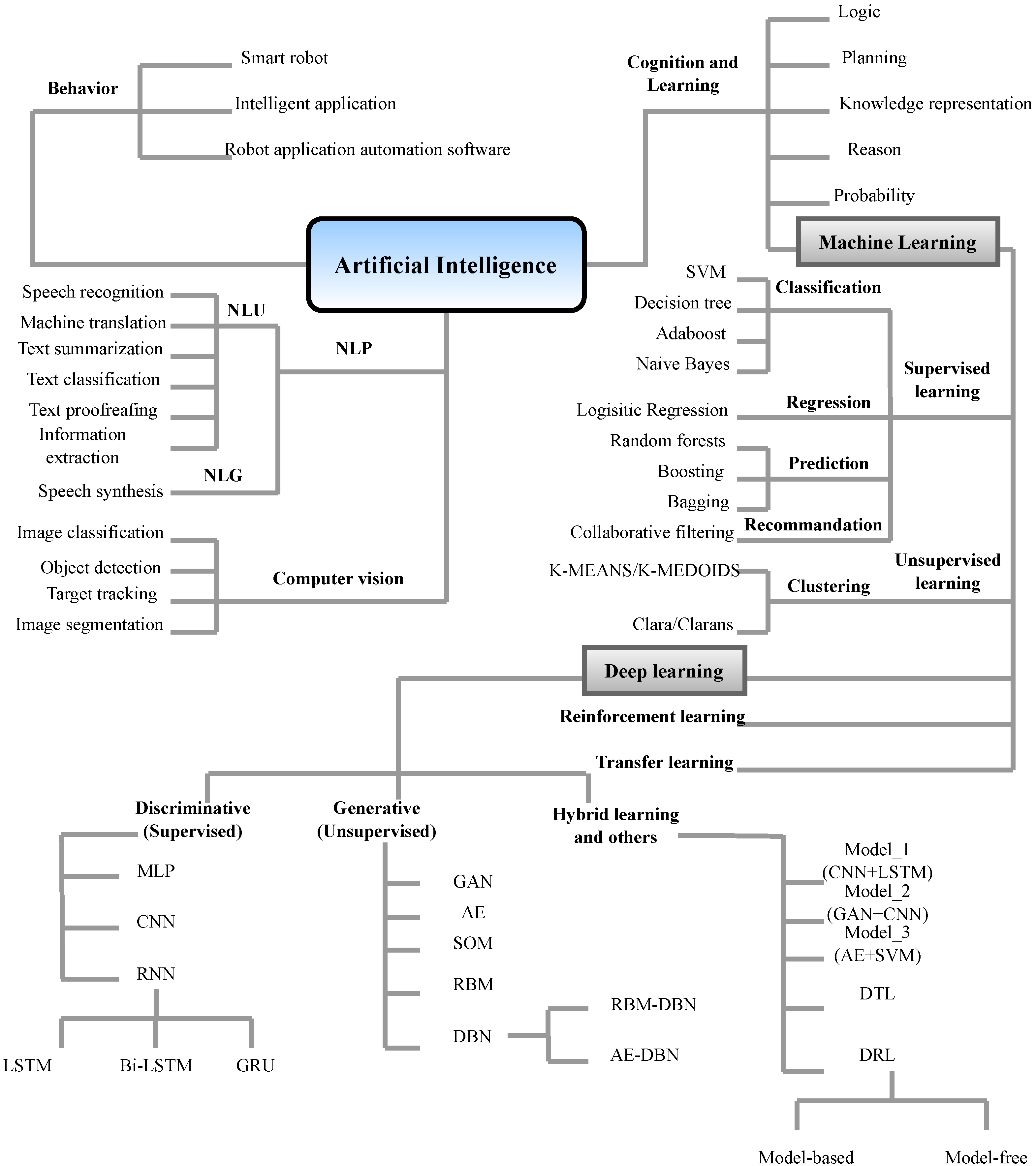
- Supervised learning: Learning from labeled training information to predict results for unseen data. Classification and regression are the most popular applications of supervised learning.
- Unsupervised learning: Labelled data are not required. Data are clustered by finding hidden patterns and relationships among data points.
- Semi-supervised learning: Refers to a type of training problem where the data set is composed of a small volume of labeled data and a large volume of unlabeled data.
- Reinforcement learning: This scheme, which is situated between supervised and unsupervised learning, provides an “agent” that has the capability to learn from its surrounding environment.
5. Future Directions
- The newest generation of sensing systems incorporates recent innovations in sensor technologies such as intelligent materials, active sensing, wireless data transfer, and deep learning, while some of these novel techniques have been applied to real structures, many have only been studied under research conditions, and they must be further explored in real-life environments for their benefits and challenges to be fully assessed and understood.
- NDT and SHM of components exposed to high temperatures (>650 °C) is a field of increasing importance. Their implementation, however, poses significant challenges due to the harsh high-temperature environments. The development of advanced sensors suitable to these environments is, therefore, an essential field of future research.
- Despite significant progress in sensing developments, many challenges remain demanding further research efforts. The next generation of smart structures is aimed to incorporate smart materials with embedded sensing power that consume only little energy or are self-powered, resist noise and environmental variations, and are cost-effective and eco-friendly.
- Novel vision-based sensors need to be insensitive to light conditions, demanding the development of improved algorithms for image processing.
- Self-sensing materials are an exciting field of research investigating strategies such as embedding fiber-optic and piezoceramic sensors in a structure’s critical components. Future research directions are aimed at developing self-sensing materials that are able to instantly identify any material changes induced by damage in the nano- or microstructure.
- Further research is needed in the field of deep learning algorithms as potential replacements or additions to traditional data analysis approaches for intelligent pattern recognition for damage identification and classification.
- Big data-driven product design is a hot topic with many ongoing developments and applications related to the Internet of things (IoT).
- Digital twin technology, which analyzes sensor data using AI algorithms, is a cutting-edge technology linking the physical and virtual worlds. More research is needed to exploit the capabilities of digital twin technology fully.
- Existing sensor technologies, such as cameras, microphones, inertial measurement units, etc., are widely used for various applications, but their high-power consumption and battery replacement remain a concern. Further developments are needed on self-powered sensors, such as using triboelectric nanogenerators (TENGs) that provide a feasible platform to realize self-sustainable and low-power systems.
6. Conclusions
Author Contributions
Funding
Institutional Review Board Statement
Informed Consent Statement
Data Availability Statement
Conflicts of Interest
References
- El Masri, Y.; Rakha, T. A scoping review of non-destructive testing (NDT) techniques in building performance diagnostic inspections. Constr. Build. Mater. 2020, 265, 120542. [Google Scholar] [CrossRef]
- Mićić, M.; Brajović, L.; Lazarević, L.; Popović, Z. Inspection of RCF rail defects–Review of NDT methods. Mech. Syst. Signal Process. 2023, 182, 109568. [Google Scholar] [CrossRef]
- Ramírez, I.S.; Márquez, F.P.G.; Papaelias, M. Review on additive manufacturing and non-destructive testing. J. Manuf. Syst. 2023, 66, 260–286. [Google Scholar] [CrossRef]
- Gagliardi, V.; Tosti, F.; Bianchini Ciampoli, L.; Battagliere, M.L.; D’Amato, L.; Alani, A.M.; Benedetto, A. Satellite remote sensing and non-destructive testing methods for transport infrastructure monitoring: Advances, challenges and perspectives. Remote Sens. 2023, 15, 418. [Google Scholar] [CrossRef]
- Perfetto, D.; De Luca, A.; Perfetto, M.; Lamanna, G.; Caputo, F. Damage Detection in Flat Panels by Guided Waves Based Artificial Neural Network Trained through Finite Element Method. Materials 2021, 14, 7602. [Google Scholar] [CrossRef]
- Lv, G.; Guo, S.; Chen, D.; Feng, H.; Zhang, K.; Liu, Y.; Feng, W. Laser ultrasonics and machine learning for automatic defect detection in metallic components. NDT E Int. 2023, 133, 102752. [Google Scholar] [CrossRef]
- Cantero-Chinchilla, S.; Wilcox, P.D.; Croxford, A.J. Deep learning in automated ultrasonic NDE—Developments, axioms and opportunities. NDT E Int. 2022, 131, 102703. [Google Scholar] [CrossRef]
- Shrifan, N.H.; Akbar, M.F.; Isa, N.A.M. Prospect of using artificial intelligence for microwave nondestructive testing technique: A review. IEEE Access 2019, 7, 110628–110650. [Google Scholar] [CrossRef]
- Schmidt, C.; Hocke, T.; Denkena, B. Artificial intelligence for non-destructive testing of CFRP prepreg materials. Prod. Eng. 2019, 13, 617–626. [Google Scholar] [CrossRef]
- Liu, Y.; Yuan, K.; Li, T.; Li, S.; Ren, Y. NDT Method for Line Laser Welding Based on Deep Learning and One-Dimensional Time-Series Data. Appl. Sci. 2022, 12, 7837. [Google Scholar] [CrossRef]
- Hassani, S.; Mousavi, M.; Gandomi, A.H. Structural Health Monitoring in Composite Structures: A Comprehensive Review. Sensors 2022, 22, 153. [Google Scholar] [CrossRef]
- Zinno, R.; Haghshenas, S.S.; Guido, G.; VItale, A. Artificial intelligence and structural health monitoring of bridges: A review of the state-of-the-art. IEEE Access 2022, 10, 88058–88078. [Google Scholar] [CrossRef]
- Sujith, A.; Sajja, G.S.; Mahalakshmi, V.; Nuhmani, S.; Prasanalakshmi, B. Systematic review of smart health monitoring using deep learning and Artificial intelligence. Neurosci. Inform. 2022, 2, 100028. [Google Scholar] [CrossRef]
- Flah, M.; Nunez, I.; Ben Chaabene, W.; Nehdi, M.L. Machine learning algorithms in civil structural health monitoring: A systematic review. Arch. Comput. Methods Eng. 2021, 28, 2621–2643. [Google Scholar] [CrossRef]
- Malekloo, A.; Ozer, E.; AlHamaydeh, M.; Girolami, M. Machine learning and structural health monitoring overview with emerging technology and high-dimensional data source highlights. Struct. Health Monit. 2022, 21, 1906–1955. [Google Scholar] [CrossRef]
- Chou, J.Y.; Fu, Y.; Huang, S.K.; Chang, C.M. SHM data anomaly classification using machine learning strategies: A comparative study. Smart Struct. Syst. 2022, 29, 77–91. [Google Scholar]
- Kraljevski, I.; Duckhorn, F.; Tschöpe, C.; Wolff, M. Machine learning for anomaly assessment in sensor networks for NDT in aerospace. IEEE Sensors J. 2021, 21, 11000–11008. [Google Scholar] [CrossRef]
- Tian, Y.G.; Zhang, Z.N.; Tian, S.Q. Nondestructive testing for wheat quality with sensor technology based on Big Data. J. Anal. Methods Chem. 2020, 2020, 8851509. [Google Scholar] [CrossRef]
- Yurchenko, A.; Mekhtiyev, A.; Bulatbayev, F.; Neshina, Y.; Alkina, A. The Model of a Fiber-Optic Sensor for Monitoring Mechanical Stresses in Mine Workings. Russ. J. Nondestruct. Test. 2018, 54, 528–533. [Google Scholar] [CrossRef]
- Wevers, M.; Rippert, L.; Van Huffel, S. Optical fibres for in situ monitoring the damage development in composites and the relation with acoustic emission measurements. J. Acoust. Emiss. 2000, 18, 41. [Google Scholar]
- Sundaresan, M.J.; Schulz, M.J.; Ghoshal, A.; Martin, W.N., Jr.; Pratap, P.R. Neural system for structural health monitoring. In Proceedings of the Smart Structures and Materials 2001: Sensory Phenomena and Measurement Instrumentation for Smart Structures and Materials, Newport Beach, CA, USA, 5–6 March 2001; Volume 4328, pp. 130–141. [Google Scholar]
- Martin, J.M.M.; Munoz-Esquer, P.; Rodriguez-Lence, F.; Guemes, J.A. Fiber optic sensors for process monitoring of composite aerospace structures. In Proceedings of the Smart Structures and Materials 2002: Smart Sensor Technology and Measurement Systems, San Diego, CA, USA, 18–19 March 2002; Volume 4694, pp. 53–64. [Google Scholar]
- Toyama, N.; Noda, J.; Okabe, T. Quantitative damage detection in cross-ply laminates using Lamb wave method. Compos. Sci. Technol. 2003, 63, 1473–1479. [Google Scholar] [CrossRef]
- Mallet, L.; Lee, B.; Staszewski, W.; Scarpa, F. Structural health monitoring using scanning laser vibrometry: II. Lamb waves for damage detection. Smart Mater. Struct. 2004, 13, 261. [Google Scholar] [CrossRef]
- Oka, M.; Yakushiji, T.; Tsuchida, Y.; Enokizono, M. Evaluation of fatigue damage in an austenitic stainless steel (SUS304) using the eddy current probe. In Proceedings of the 2005 IEEE International Magnetics Conference (INTERMAG), Nagoya, Japan, 4–8 April 2005; pp. 427–428. [Google Scholar]
- Tsuda, H. Ultrasound and damage detection in CFRP using fiber Bragg grating sensors. Compos. Sci. Technol. 2006, 66, 676–683. [Google Scholar] [CrossRef]
- Yashiro, S.; Takatsubo, J.; Toyama, N. An NDT technique for composite structures using visualized Lamb-wave propagation. Compos. Sci. Technol. 2007, 67, 3202–3208. [Google Scholar] [CrossRef]
- Yu, T.Y.; Büyüköztürk, O. A far-field airborne radar NDT technique for detecting debonding in GFRP–retrofitted concrete structures. NDT E Int. 2008, 41, 10–24. [Google Scholar] [CrossRef]
- Meitzler, T.J.; Wong, I.; Bryk, D.; Reynolds, T.; Ebenstein, S. Damage Detection in Composite Plate Armor Using Ultrasonic Techniques; Technical Report, Army Tank-Automotive Command Warren Mi Survivability Research Div; US Army RDECOM-TARDEC: Warren, MI, USA, 2009. [Google Scholar]
- Güemes, A.; Fernandez-Lopez, A. Damage detection in bolted joints by fibre optics distributed sensing. In Proceedings of the 2nd International Symposium on NDT in Aerospace, Williamsburg, VA, USA, 5–7 October 2010; Number 1, pp. 14–20. [Google Scholar]
- Zhou, J. A study of Acoustic Emission Technique for Concrete Damage Detection. Master’s Report, Michigan Technological University, Houghton, MI, USA, 2011; pp. 14–20. [Google Scholar]
- Amaro, A.; Reis, P.; De Moura, M.; Santos, J. Damage detection on laminated composite materials using several NDT techniques. Insight-Non-Destr. Test. Cond. Monit. 2012, 54, 14–20. [Google Scholar] [CrossRef]
- Cuadra, J.; Vanniamparambil, P.A.; Hazeli, K.; Bartoli, I.; Kontsos, A. Damage quantification in polymer composites using a hybrid NDT approach. Compos. Sci. Technol. 2013, 83, 11–21. [Google Scholar] [CrossRef]
- Ye, G.; Neal, B.; Boot, A.; Kappatos, V.; Selcuk, C.; Gan, T.H. Development of an ultrasonic NDT system for automated in situ inspection of wind turbine blades. In Proceedings of the EWSHM-7th European Workshop on Structural Health Monitoring, Nantes, France, 8–11 July 2014. [Google Scholar]
- Song, Y.; Wu, F. Rail Damage Detection Based on AE Technology and Wavelet Data Processing. Appl. Mech. Mater. Trans. Tech. Publ. 2015, 744, 1339–1343. [Google Scholar] [CrossRef]
- Wang, D.; He, J.; Dong, B.; Liu, X.; Zhang, W. Novel damage detection techniques for structural health monitoring using a hybrid sensor. Math. Probl. Eng. 2016, 2016, 3734258. [Google Scholar] [CrossRef] [Green Version]
- Moriot, J.; Quaegebeur, N.; Le Duff, A.; Masson, P. Model-Assisted Assessment of Damage Detection and Localization Using Guided Wave-Based Imaging Techniques. Struct. Health Monit. 2017, 17, 1460–1472. [Google Scholar] [CrossRef] [Green Version]
- Yang, K.; Rongong, J.A.; Worden, K. Damage detection in a laboratory wind turbine blade using techniques of ultrasonic NDT and SHM. Strain 2018, 54, e12290. [Google Scholar] [CrossRef]
- Rathod, H.; Gupta, R. Sub-surface simulated damage detection using Non-Destructive Testing Techniques in reinforced-concrete slabs. Constr. Build. Mater. 2019, 215, 754–764. [Google Scholar] [CrossRef]
- Rittmann, J.; Rahammer, M.; Holtmann, N.; Kreutzbruck, M. A mobile nondestructive testing (NDT) system for fast detection of impact damage in fiber-reinforced plastics (FRP). J. Sensors Sens. Syst. 2020, 9, 43–50. [Google Scholar] [CrossRef]
- Ni, Q.Q.; Hong, J.; Xu, P.; Xu, Z.; Khvostunkov, K.; Xia, H. Damage detection of CFRP composites by electromagnetic wave nondestructive testing (EMW-NDT). Compos. Sci. Technol. 2021, 210, 108839. [Google Scholar] [CrossRef]
- Chakraborty, J.; Stolinski, M. Signal-Level Fusion Approach for Embedded Ultrasonic Sensors in Damage Detection of Real RC Structures. Mathematics 2022, 10, 724. [Google Scholar] [CrossRef]
- Kim, D.; Kim, R.; Min, J.; Choi, H. Initial freeze—Thaw damage detection in concrete using two-dimensional non-contact ultrasonic sensors. Constr. Build. Mater. 2023, 364, 129854. [Google Scholar] [CrossRef]
- Howard, J.; Murashov, V.; Cauda, E.; Snawder, J. Advanced sensor technologies and the future of work. Am. J. Ind. Med. 2022, 65, 3–11. [Google Scholar] [CrossRef]
- IMARC Group. Structural Health Monitoring Market: Global Industry Trends, Share, Size, Growth, Opportunity and Forecast 2022–2027; IMARC Group: Noida, India, 2022; 145p. [Google Scholar]
- Panwar, N.G.; Singh, S.; Garg, A.; Gupta, A.K.; Gao, L. Recent Advancements in Battery Management System for Li-Ion Batteries of Electric Vehicles: Future Role of Digital Twin, Cyber-Physical Systems, Battery Swapping Technology, and Nondestructive Testing. Energy Technol. 2021, 9, 2000984. [Google Scholar] [CrossRef]
- Towsyfyan, H.; Biguri, A.; Boardman, R.; Blumensath, T. Successes and challenges in non-destructive testing of aircraft composite structures. Chin. J. Aeronaut. 2020, 33, 771–791. [Google Scholar] [CrossRef]
- Ma, Q.; Tian, G.; Zeng, Y.; Li, R.; Song, H.; Wang, Z.; Gao, B.; Zeng, K. Pipeline in-line inspection method, instrumentation and data management. Sensors 2021, 21, 3862. [Google Scholar] [CrossRef]
- Malik, M.S. Model assisted POD of laser-ultrasonics NDT for train axles: A review. In Proceedings of the 2016 International Conference on Electrical, Electronics, and Optimization Techniques (ICEEOT), Chennai, India, 3–5 March 2016; pp. 4645–4648. [Google Scholar]
- Gupta, M.; Khan, M.A.; Butola, R.; Singari, R.M. Advances in applications of Non-Destructive Testing (NDT): A review. Adv. Mater. Process. Technol. 2022, 8, 2286–2307. [Google Scholar] [CrossRef]
- Khedmatgozar Dolati, S.S.; Caluk, N.; Mehrabi, A.; Khedmatgozar Dolati, S.S. Non-Destructive Testing Applications for Steel Bridges. Appl. Sci. 2021, 11, 9757. [Google Scholar] [CrossRef]
- Wooldridge, A. Recent advances in automated ultrasonic inspection of Magnox power stations. Mater. Test. 2007, 49, 290–298. [Google Scholar] [CrossRef] [Green Version]
- Lovejoy, M. Magnetic Particle Inspection: A Practical Guide; Springer Science & Business Media: Berlin/Heidelberg, Germany, 1993. [Google Scholar]
- Mustapha, S.; Lu, Y.; Ng, C.T.; Malinowski, P. Sensor networks for structures health monitoring: Placement, implementations, and challenges—A review. Vibration 2021, 4, 551–585. [Google Scholar] [CrossRef]
- Shokravi, H.; Shokravi, H.; Bakhary, N.; Rahimian Koloor, S.S.; Petrů, M. Health monitoring of civil infrastructures by subspace system identification method: An overview. Appl. Sci. 2020, 10, 2786. [Google Scholar] [CrossRef] [Green Version]
- Teng, S.; Chen, X.; Chen, G.; Cheng, L.; Bassir, D. Structural damage detection based on convolutional neural networks and population of bridges. Measurement 2022, 202, 111747. [Google Scholar] [CrossRef]
- Vega, M.A.; Hu, Z.; Fillmore, T.B.; Smith, M.D.; Todd, M.D. A novel framework for integration of abstracted inspection data and structural health monitoring for damage prognosis of miter gates. Reliab. Eng. Syst. Saf. 2021, 211, 107561. [Google Scholar] [CrossRef]
- Junyan, L.; Yang, L.; Fei, W.; Yang, W. Study on probability of detection (POD) determination using lock-in thermography for nondestructive inspection (NDI) of CFRP composite materials. Infrared Phys. Technol. 2015, 71, 448–456. [Google Scholar] [CrossRef]
- Hübschen, G.; Altpeter, I.; Tschuncky, R.; Herrmann, H.G. Materials Characterization Using Nondestructive Evaluation (NDE) Methods; Woodhead Publishing: Soston, UK, 2016. [Google Scholar]
- Bray, D.E.; Stanley, R.K. Nondestructive Evaluation: A Tool in Design, Manufacturing, and Service; CRC Press: Boca Raton, FL, USA, 2018. [Google Scholar]
- Yang, R.; He, Y.; Zhang, H. Progress and trends in nondestructive testing and evaluation for wind turbine composite blade. Renew. Sustain. Energy Rev. 2016, 60, 1225–1250. [Google Scholar] [CrossRef]
- Honarvar, F.; Varvani-Farahani, A. A review of ultrasonic testing applications in additive manufacturing: Defect evaluation, material characterization, and process control. Ultrasonics 2020, 108, 106227. [Google Scholar] [CrossRef]
- Amiri, N.; Farrahi, G.; Kashyzadeh, K.R.; Chizari, M. Applications of ultrasonic testing and machine learning methods to predict the static & fatigue behavior of spot-welded joints. J. Manuf. Process. 2020, 52, 26–34. [Google Scholar]
- Lehmann, E.H.; Ridikas, D.; Barradas, N.P. What Future in Neutron Imaging? Neutron Radiogr. WCNR-11 2020, 15, 3. [Google Scholar]
- Saeedifar, M.; Zarouchas, D. Damage characterization of laminated composites using acoustic emission: A review. Compos. Part B Eng. 2020, 195, 108039. [Google Scholar] [CrossRef]
- Sahu, M.K.; Sagar, S.P. Nonlinearity in the propagation of acoustic waves: Simulation and experimental validation in a creep damaged material. Mater. Today Proc. 2021, 44, 2251–2256. [Google Scholar] [CrossRef]
- Górszczyk, J.; Malicki, K.; Zych, T. Application of digital image correlation (DIC) method for road material testing. Materials 2019, 12, 2349. [Google Scholar] [CrossRef] [Green Version]
- Escauriza, E.M.; Olbinado, M.P.; Rutherford, M.E.; Chapman, D.J.; Jonsson, J.C.; Rack, A.; Eakins, D.E. Ultra-high-speed indirect X-ray imaging system with versatile spatiotemporal sampling capabilities. Appl. Optics 2018, 57, 5004–5010. [Google Scholar] [CrossRef]
- Sen, S.; Abdullah-Al-Shafi, M.; Sikder, A.S.; Hossain, M.S.; Azad, M.M. Zeonex based decagonal photonic crystal fiber (D-PCF) in the terahertz (THz) band for chemical sensing applications. Sens. Bio-Sens. Res. 2021, 31, 100393. [Google Scholar] [CrossRef]
- Varma, C.M. Colloquium: Linear in temperature resistivity and associated mysteries including high temperature superconductivity. Rev. Mod. Phys. 2020, 92, 031001. [Google Scholar] [CrossRef]
- Kirimtat, A.; Krejcar, O. A review of infrared thermography for the investigation of building envelopes: Advances and prospects. Energy Build. 2018, 176, 390–406. [Google Scholar] [CrossRef]
- Gatto, V.; Anisimov, A.G.; Lettinga, W.; Tao, N.; Lantman, M.; Crijns, B.; Groves, R.M. Application of shearography and the percussion method for the structural inspection of wall paintings: A case study of St. Christopher in Maria Church, Nisse. In Proceedings of the Optics for Arts, Architecture, and Archaeology VIII, Online Only, 21–25 June 2021; Volume 11784, pp. 87–94. [Google Scholar]
- Joubert, J.M. Intermetallic compounds of the Cr–Mn system investigated using in situ powder neutron diffraction: The reported order-disorder transformation of the σ phase elucidated. Intermetallics 2022, 146, 107580. [Google Scholar] [CrossRef]
- AbdAlla, A.N.; Faraj, M.A.; Samsuri, F.; Rifai, D.; Ali, K.; Al-Douri, Y. Challenges in improving the performance of eddy current testing. Meas. Control 2019, 52, 46–64. [Google Scholar] [CrossRef] [Green Version]
- Park, S.H.; Choi, S.; Jhang, K.Y. Porosity evaluation of additively manufactured components using deep learning-based ultrasonic nondestructive testing. Int. J. Precis. Eng. Manuf. Green Technol. 2022, 9, 395–407. [Google Scholar] [CrossRef]
- Taheri, H.; Jones, C.; Taheri, M. Assessment and detection of stress corrosion cracking by advanced eddy current array nondestructive testing and material characterization. J. Nat. Gas Sci. Eng. 2022, 102, 104568. [Google Scholar] [CrossRef]
- Zhang, J.; Cho, Y.; Kim, J.; Malikov, A.K.U.; Kim, Y.H.; Yi, J.H.; Li, W. Non-Destructive Evaluation of Coating Thickness Using Water Immersion Ultrasonic Testing. Coatings 2021, 11, 1421. [Google Scholar] [CrossRef]
- Pan, Z.; Zhou, W.; Zhang, K.; Ma, L.; Liu, J. Flexural damage and failure behavior of 3D printed continuous fiber composites by complementary nondestructive testing technology. Polym. Compos. 2022, 43, 2864–2877. [Google Scholar] [CrossRef]
- Awoyera, P.O.; Olalusi, O.B. Modeling Temperature of Fire-Damaged Reinforced Concrete Buildings Based on Nondestructive Testing and Gene Algorithm Techniques. Fire Technol. 2022, 58, 941–957. [Google Scholar] [CrossRef]
- Zheng, Y.; Wang, S.; Zhang, P.; Xu, T.; Zhuo, J. Application of Nondestructive Testing Technology in Quality Evaluation of Plain Concrete and RC Structures in Bridge Engineering: A Review. Buildings 2022, 12, 843. [Google Scholar] [CrossRef]
- Lee, J.; Lee, H.; Berkache, A. Novel Approaches for Nondestructive Testing and Evaluation. Appl. Sci. 2022, 12, 565. [Google Scholar] [CrossRef]
- Asif, M.; Khan, M.A.; Khan, S.Z.; Choudhry, R.S.; Khan, K.A. Identification of an effective nondestructive technique for bond defect determination in laminate composites—A technical review. J. Compos. Mater. 2018, 52, 3589–3599. [Google Scholar] [CrossRef] [Green Version]
- Ke, Q.; Li, W.; Wang, W.; Song, S. Correction method with stress field effects in ultrasound nondestructive testing. Nondestruct. Test. Eval. 2022, 37, 277–296. [Google Scholar] [CrossRef]
- Yang, N.; Wang, Z. Influence of number and position of measuring points on the nondestructive testing method to predict the flexural modulus of aged wood. Holzforschung 2022, 76, 421–429. [Google Scholar] [CrossRef]
- Ewald, V.; Goby, X.; Jansen, H.; Groves, R.M.; Benedictus, R. Incorporating inductive bias into deep learning: A perspective from automated visual inspection in aircraft maintenance. In Proceedings of the 10th International Symposium on NDT in Aerospace, Dresden, Germany, 24–26 October 2018; pp. 1–9. [Google Scholar]
- Yasuda, Y.D.; Cappabianco, F.A.; Martins, L.E.G.; Gripp, J.A. Aircraft visual inspection: A systematic literature review. Comput. Ind. 2022, 141, 103695. [Google Scholar] [CrossRef]
- Grinzato, E.; Bressan, C.; Marinetti, S.; Bison, P.; Bonacina, C. Monitoring of the Scrovegni Chapel by IR thermography: Giotto at infrared. Infrared Phys. Technol. 2002, 43, 165–169. [Google Scholar] [CrossRef]
- Gholizadeh, S.; Leman, Z.; Baharudin, B.H.T. A review of the application of acoustic emission technique in engineering. Struct. Eng. Mech. 2015, 54, 1075–1095. [Google Scholar] [CrossRef]
- Gao, P.; Wang, C.; Li, Y.; Cong, Z. Electromagnetic and eddy current NDT in weld inspection: A review. Insight-Non-Destr. Test. Cond. Monit. 2015, 57, 337–345. [Google Scholar] [CrossRef]
- Endramawan, T.; Haris, E.; Dionisius, F.; Prinka, Y. Aplikasi Non Destructive Test Penetrant Testing (Ndt-Pt) Untuk Analisis Hasil Pengelasan Smaw 3g Butt Joint. J. Teknol. Ter. 2017, 3, 44–48. [Google Scholar] [CrossRef]
- Roshan, C.C.; Raghul, C.; Ram, H.V.; Suraj, K.; Solomon, J. Non-destructive testing by liquid penetrant testing and ultrasonic testing—A review. Int. J. Adv. Res. Ideas Innov. Technol. 2019, 5, 694–697. [Google Scholar]
- Wilkinson, S.; Duke, S.M. Comparative Testing of Radiographic Testing, Ultrasonic Testing and Phased Array Advanced Ultrasonic Testing non Destructive Testing Techniques in Accordance with the AWS D1. 5 Bridge Welding Code; Technical Report; Florida Department of Transportation: Tallahassee, FL, USA, 2014.
- Chen, Y.; Kang, Y.; Feng, B.; Li, Y.; Cai, X.; Wang, S. Automatic Defect Identification in Magnetic Particle Testing Using a Digital Model Aided De-noising Method. Measurement 2022, 198, 111427. [Google Scholar] [CrossRef]
- Wang, B.; He, P.; Kang, Y.; Jia, J.; Liu, X.; Li, N. Ultrasonic Testing of Carbon Fiber-Reinforced Polymer Composites. J. Sensors 2022, 2022, 5462237. [Google Scholar] [CrossRef]
- Márquez, F.P.G.; Chacón, A.M.P. A review of non-destructive testing on wind turbines blades. Renew. Energy 2020, 161, 998–1010. [Google Scholar] [CrossRef]
- Dackermann, U.; Elsener, R.; Li, J.; Crews, K. A comparative study of using static and ultrasonic material testing methods to determine the anisotropic material properties of wood. Constr. Build. Mater. 2016, 102, 963–976. [Google Scholar] [CrossRef]
- Zscherpel, U.; Ewert, U.; Bavendiek, K.; Jechow, M. Strategies for Film Replacement in Radiography-Approaches Used in the New Standards. In Proceedings of the International Symposium on Digital Industrial Radiology and Computed Tomography, Berlin, Germany, 20–22 June 2011; pp. 20–22. [Google Scholar]
- Shaikh, H.; Sivaibharasi, N.; Sasi, B.; Anita, T.; Amirthalingam, R.; Rao, B.; Jayakumar, T.; Khatak, H.; Raj, B. Use of eddy current testing method in detection and evaluation of sensitisation and intergranular corrosion in austenitic stainless steels. Corros. Sci. 2006, 48, 1462–1482. [Google Scholar] [CrossRef]
- Mohammed, S. NDT and SHM Methods of Damage Detection in Welded Structures. Ph.D. Thesis, University of South Carolina, Columbia, SC, USA, 2016. [Google Scholar]
- Lvovsky, O.; Grayson, C.M. Aerospace Payloads Leak Test Methodology. In Proceedings of the American Society for Nondestructive Testing (ASNT) Fall Conference, Houston, TX, USA, 15–19 November 2010. number JSC-CN-21358. [Google Scholar]
- Peng, X.; Anyaoha, U.; Liu, Z.; Tsukada, K. Analysis of magnetic-flux leakage (MFL) data for pipeline corrosion assessment. IEEE Trans. Magn. 2020, 56, 1–15. [Google Scholar] [CrossRef]
- Alobaidi, W.M.; Sandgren, E. High-Efficiency Remote Measurement of Pipe Defect Using RF/UT Technologies: A Theoretical Analysis Part One—Straight Beam UT. In Proceedings of the Pressure Vessels and Piping Conference. American Society of Mechanical Engineers, New York, NY, USA, 17–21 July 2016; Volume 50411, p. V005T10A006. [Google Scholar]
- Low, C.; Wong, B. Defect evaluation using the alternating current field measurement technique. Insight-Non-Destr. Test. Cond. Monit. 2004, 46, 598–605. [Google Scholar] [CrossRef]
- Ahmed, S.R.; Saka, M. Quantitative nondestructive testing of small, tight cracks using ultrasonic angle beam technique. Mater. Eval. 2000, 58, 564–574. [Google Scholar]
- Singh, D.K.; Singh, B.; Malhotra, A. A Study on Microwave Absorption and Ultrasonic Techniques with Different Liquid Polymer.
- Junkin, G.; Huang, T.; Bennett, J.C. Holographic testing of terahertz antennas. IEEE Trans. Antennas Propag. 2000, 48, 409–417. [Google Scholar] [CrossRef]
- Zhao, Q.; Dan, X.; Sun, F.; Wang, Y.; Wu, S.; Yang, L. Digital shearography for NDT: Phase measurement technique and recent developments. Appl. Sci. 2018, 8, 2662. [Google Scholar] [CrossRef] [Green Version]
- Beránek, L.; Kroisová, D.; Dvořáčková, Š.; Urban, J.; Šimota, J.; Andronov, V.; Bureš, L.; Pelikán, L. Use of computed tomography in dimensional quality control and NDT. Manuf. Technol. 2020, 20, 566–575. [Google Scholar] [CrossRef]
- Gao, Y.; Song, G.; Li, S.; Zhen, F.; Chen, D.; Song, A. LineSpyX: A power line inspection robot based on digital radiography. IEEE Robot. Autom. Lett. 2020, 5, 4759–4765. [Google Scholar] [CrossRef]
- Song, J.I.; Kim, H.S. Preliminary study (1) for development of computed radiography (CR) image analysis according to X-ray non-destructive test by wood species. J. Conserv. Sci. 2021, 37, 220–231. [Google Scholar] [CrossRef]
- Guo, W.; Gao, B.; Yun Tian, G.; Si, D. Physic perspective fusion of electromagnetic acoustic transducer and pulsed eddy current testing in non-destructive testing system. Philos. Trans. R. Soc. A 2020, 378, 20190608. [Google Scholar] [CrossRef] [PubMed]
- Mayworm, R.; Alvarenga, A.; Costa-Felix, R. A metrological approach to the time of flight diffraction method (ToFD). Measurement 2021, 167, 108298. [Google Scholar] [CrossRef]
- Yilmaz, B.; Asokkumar, A.; Jasiūnienė, E.; Kažys, R.J. Air-coupled, contact, and immersion ultrasonic non-destructive testing: Comparison for bonding quality evaluation. Appl. Sci. 2020, 10, 6757. [Google Scholar] [CrossRef]
- Nadzri, M.M.M.; Ahmad, A. Design Issues and Challenges of Long-Range Ultrasonic Testing (LRUT) for Pipeline Inspection. In Proceedings of the 12th National Technical Seminar on Unmanned System Technology 2020, 27–28 October 2022; pp. 115–126. [Google Scholar]
- Saffiudeen, M.F.; Syed, A.; Mohammed, F.T. Failure Analysis of Heat Exchanger Using Internal Rotary Inspection System (IRIS). J. Fail. Anal. Prev. 2021, 21, 494–498. [Google Scholar] [CrossRef]
- Taheri, H.; Hassen, A.A. Nondestructive ultrasonic inspection of composite materials: A comparative advantage of phased array ultrasonic. Appl. Sci. 2019, 9, 1628. [Google Scholar] [CrossRef] [Green Version]
- Pan, Y.; Molin, Q.; Guo, T.; Zhang, L.; Cao, B.; Yang, J.; Wang, W.; Xue, X. Wireless passive surface acoustic wave (SAW) technology in gas sensing. Sens. Rev. 2021, 41, 135–143. [Google Scholar] [CrossRef]
- Brigante, M.; Sumbatyan, M. Acoustic methods for the nondestructive testing of concrete: A review of foreign publications in the experimental field. Russ. J. Nondestruct. Test. 2013, 49, 100–111. [Google Scholar] [CrossRef]
- Perfetto, D.; Lamanna, G.; Petrone, G.; De Fenza, A.; De Luca, A. A modelling technique to investigate the effects of quasi-static loads on guided-wave based structural health monitoring systems. Forces Mech. 2022, 9, 100125. [Google Scholar] [CrossRef]
- Perfetto, D.; Khodaei, Z.S.; De Luca, A.; Aliabadi, M.; Caputo, F. Experiments and modelling of ultrasonic waves in composite plates under varying temperature. Ultrasonics 2022, 126, 106820. [Google Scholar] [CrossRef]
- Dackermann, U.; Crews, K.; Kasal, B.; Li, J.; Riggio, M.; Rinn, F.; Tannert, T. In situ assessment of structural timber using stress-wave measurements. Mater. Struct. 2014, 47, 787–803. [Google Scholar] [CrossRef]
- Krause, M.; Dackermann, U.; Li, J. Elastic wave modes for the assessment of structural timber: Ultrasonic echo for building elements and guided waves for pole and pile structures. J. Civ. Struct. Health Monit. 2015, 5, 221–249. [Google Scholar] [CrossRef] [Green Version]
- Liu, S.; Sun, Y.; Gu, M.; Liu, C.; He, L.; Kang, Y. Review and analysis of three representative electromagnetic NDT methods. Insight-Non-Destr. Test. Cond. Monit. 2017, 59, 176–183. [Google Scholar] [CrossRef]
- Wang, Z.; Gu, Y.; Wang, Y. A review of three magnetic NDT technologies. J. Magn. Magn. Mater. 2012, 324, 382–388. [Google Scholar] [CrossRef]
- Blitz, J. Electrical and Magnetic Methods of Non-Destructive Testing; Springer Science & Business Media: Berlin/Heidelberg, Germany, 1997; Volume 3. [Google Scholar]
- Zhu, Y.K.; Tian, G.Y.; Lu, R.S.; Zhang, H. A review of optical NDT technologies. Sensors 2011, 11, 7773–7798. [Google Scholar] [CrossRef] [PubMed] [Green Version]
- Liu, M.; Li, X. Mechanical properties measurement of materials and devices at micro-and nano-scale by optical methods: A review. Opt. Lasers Eng. 2022, 150, 106853. [Google Scholar] [CrossRef]
- Kroworz, A.; Katunin, A. Non-destructive testing of structures using optical and other methods: A review. Struct. Durab. Health Monit. 2018, 12, 1. [Google Scholar]
- Focke, O.; Hildebrand, A.; Von Kopylow, C.; Calomfirescu, M. Inspection of lamb waves in carbon fiber composites using shearographic interferometry. In Proceedings of the Nondestructive Characterization for Composite Materials, Aerospace Engineering, Civil Infrastructure, and Homeland Security 2008, San Diego, CA, USA, 11–13 March 2008; Volume 6934, pp. 20–31. [Google Scholar]
- Kriesz, H. Radiographic NDT—A review. NDT Int. 1979, 12, 270–273. [Google Scholar] [CrossRef]
- Klochkov, N.; Zverkov, I.; Kurlaev, N.; Soliman, M.S.A. Improvement of non-destructive testing methods in diagnostics of composite honeycomb structures of civil aircraft. In Proceedings of the AIP Conference Proceedings, 2021; Volume 2402, p. 020045. [Google Scholar]
- Robles, K.P.V.; Yee, J.J.; Kee, S.H. Electrical Resistivity Measurements for Nondestructive Evaluation of Chloride-Induced Deterioration of Reinforced Concrete—A Review. Materials 2022, 15, 2725. [Google Scholar] [CrossRef]
- Chen, L.; Liu, Y.; Zhang, S. Electrochemical Reduction of Cr (VI) Using a Graphene-Modified Stainless Steel Electrode. J. Electrochem. Soc. 2022, 169, 082511. [Google Scholar] [CrossRef]
- Wei, Y.; Yang, N.; Huang, K.; Wan, J.; You, F.; Yu, R.; Feng, S.; Wang, D. Steering hollow multishelled structures in photocatalysis: Optimizing surface and mass transport. Adv. Mater. 2020, 32, 2002556. [Google Scholar] [CrossRef]
- Climent, M.Á.; Miró, M.; Eiras, J.N.; Poveda, P.; de Vera, G.; Segovia, E.G.; Ramis, J. Early Detection of Corrosion-Induced Concrete Micro-cracking by Using Nonlinear Ultrasonic Techniques: Possible Influence of Mass Transport Processes. Corros. Mater. Degrad. 2022, 3, 235–257. [Google Scholar] [CrossRef]
- Sharma, G.J.; Ramani, V.N. Role of Collisional Interaction Between Helium Molecules and Background Air Molecules in the NDT Helium Leak Testing Method in Vacuum. In Advances in Non Destructive Evaluation; Springer: Berlin/Heidelberg, Germany, 2022; pp. 287–294. [Google Scholar]
- Al-Sabah, S.; Sourav, S.N.A.; McNally, C. The post-installed screw pull-out test: Development of a method for assessing in situ concrete compressive strength. J. Build. Eng. 2021, 33, 101658. [Google Scholar] [CrossRef]
- Madandoust, R.; Kazemi, M. Numerical analysis of break-off test method on concrete. Constr. Build. Mater. 2017, 151, 487–493. [Google Scholar] [CrossRef]
- Yusa, N.; Shishido, H.; Hashizume, H. Evaluating the iII-posedness of inverse problem to size flaws from eddy current NDT signals obtained with an absolute type probe. Appl. Mech. Mater. Trans. Tech. Publ. 2014, 619, 337–341. [Google Scholar] [CrossRef]
- Husby, K.; Johnsen, C.E.; Ringset, V. Presenting a novel NDT Eddy Current probe for crack detection on rough welds and steel with variable permeability. In Proceedings of the 2022 IEEE Sensors Applications Symposium (SAS), Sundsvall, Sweden, 1–3 August 2022; pp. 1–6. [Google Scholar]
- Rohkohl, E.; Kraken, M.; Schönemann, M.; Breuer, A.; Herrmann, C. How to characterize a NDT method for weld inspection in battery cell manufacturing using deep learning. Int. J. Adv. Manuf. Technol. 2022, 119, 4829–4843. [Google Scholar] [CrossRef]
- Sumanan; Kumar, A. Phased array ultrasonic imaging using angle beam virtual source full matrix capture-total focusing method. NDT E Int. 2020, 116, 102324. [Google Scholar] [CrossRef]
- Ducousso, M.; Reverdy, F. Real-time imaging of microcracks on metallic surface using total focusing method and plane wave imaging with Rayleigh waves. NDT E Int. 2020, 116, 102311. [Google Scholar] [CrossRef]
- Kumar, N.P.; Patankar, V. Design and development of water-immersible two-channel high-voltage spike pulser for under-water inspection and gauging of pipes. Rev. Sci. Instruments 2022, 93, 014703. [Google Scholar] [CrossRef]
- Ulapane, N.; Alempijevic, A.; Miro, J.V.; Vidal-Calleja, T. Non-destructive evaluation of ferromagnetic material thickness using pulsed eddy current sensor detector coil voltage decay rate. NDT E Int. 2018, 100, 108–114. [Google Scholar] [CrossRef]
- Xi, Z.; Luo, X.; Peng, Y.; Wang, X. Simulation and performance study of circular ultrasonic array for tubes’ internal inspection. Ultrasonics 2021, 116, 106508. [Google Scholar] [CrossRef]
- She, S.; Chen, Y.; He, Y.; Zou, X. Optimal design of remote field eddy current testing probe for ferromagnetic pipeline inspection. Measurement 2021, 168, 108306. [Google Scholar] [CrossRef]
- Jiang, S.; Lu, X.; Wang, H.; Song, K.; Jiang, Y. Simulation and experimental study of remote field current testing for hidden defects of aluminum alloy plate with damping coating. Sens. Rev. 2022, 42, 365–375. [Google Scholar] [CrossRef]
- Sacarea, A.I.; Oancea, G.; Parv, L. Magnetic Particle Inspection Optimization Solution within the Frame of NDT 4.0. Processes 2021, 9, 1067. [Google Scholar] [CrossRef]
- Biruu, F.; Sexton, J.; Liang, C.W.; Missous, M. An Automated Two-Dimensional Magnetic Field Scanner based on Quantum Well Hall Effect Sensor for Non-Destructive Testing. In Proceedings of the British Institute for Non-Destructive Testing, 57th Annual British Conference, Nottingham, UK, 10–12 September 2018. [Google Scholar]
- Moskovchenko, A.; Vavilov, V.; Švantner, M.; Muzika, L.; Houdková, Š. Active IR thermography evaluation of coating thickness by determining apparent thermal effusivity. Materials 2020, 13, 4057. [Google Scholar] [CrossRef] [PubMed]
- Wang, Y.; Fan, M.; Cao, B.; Ye, B.; Wen, D. Measurement of coating thickness using lift-off point of intersection features from pulsed eddy current signals. NDT E Int. 2020, 116, 102333. [Google Scholar] [CrossRef]
- Craeye, B.; Van De Laar, H.; van der Eijk, J.; Gijbels, W.; Lauriks, L. On-site strength assessment of limestone based concrete slabs by combining non-destructive techniques. J. Build. Eng. 2017, 13, 216–223. [Google Scholar] [CrossRef]
- Helal, J.; Sofi, M.; Mendis, P. Non-destructive testing of concrete: A review of methods. Electron. J. Struct. Eng. 2015, 14, 97–105. [Google Scholar] [CrossRef]
- Breysse, D.; Martínez-Fernández, J.L. Assessing concrete strength with rebound hammer: Review of key issues and ideas for more reliable conclusions. Mater. Struct. 2014, 47, 1589–1604. [Google Scholar] [CrossRef]
- Brozovsky, J. High-strength concrete—NDT with rebound hammer: Influence of aggregate on test results. Nondestruct. Test. Eval. 2014, 29, 255–268. [Google Scholar] [CrossRef]
- Nowak, T.P.; Jasieńko, J.; Hamrol-Bielecka, K. In situ assessment of structural timber using the resistance drilling method–Evaluation of usefulness. Constr. Build. Mater. 2016, 102, 403–415. [Google Scholar] [CrossRef]
- Niemz, P.; Mannes, D. Non-destructive testing of wood and wood-based materials. J. Cult. Herit. 2012, 13, S26–S34. [Google Scholar] [CrossRef]
- Zielińska, M.; Rucka, M. Non-destructive Testing of Wooden Elements. In Proceedings of the IOP Conference Series: Materials Science and Engineering, Sanya, China, 12–14 November 2021; Volume 1203, p. 032058. [Google Scholar]
- Franke, S.; Franke, B.; Scharmacher, F. Assessment of timber structures using the X-ray technology. Adv. Mater. Res. 2013, 778, 321–327. [Google Scholar] [CrossRef]
- Dehui, W.; Fan, Y.; Teng, W.; Chen, W. A novel electromagnetic nondestructive testing method for carbon fiber reinforced polymer laminates based on power loss. Compos. Struct. 2021, 276, 114421. [Google Scholar] [CrossRef]
- Gholizadeh, S. A review of non-destructive testing methods of composite materials. Procedia Struct. Integr. 2016, 1, 50–57. [Google Scholar] [CrossRef] [Green Version]
- De Angelis, G.; Meo, M.; Almond, D.P.; Pickering, S.G.; Angioni, S.L. A new technique to detect defect size and depth in composite structures using digital shearography and unconstrained optimization. NDT E Int. 2012, 45, 91–96. [Google Scholar] [CrossRef]
- Gryzagoridis, J.; Findeis, D. Benchmarking shearographic NDT for composites. Insight-Non-Destr. Test. Cond. Monit. 2008, 50, 249–252. [Google Scholar] [CrossRef] [Green Version]
- Łątka, D.; Matysek, P. The estimation of compressive stress level in brick masonry using the flat-jack method. Procedia Eng. 2017, 193, 266–272. [Google Scholar] [CrossRef]
- Armanasco, A.; Foppoli, D. A flat jacks method for in situ testing of brick masonry shear characteristics. Constr. Build. Mater. 2020, 262, 119840. [Google Scholar] [CrossRef]
- Ercan, E.; Alver, N.; Nuhoğlu, A. Evaluation of material properties by NDT methods and FEM analysis of a stone masonry arch bridge. Chall. J. Struct. Mech. 2015, 1, 168–172. [Google Scholar]
- Alarcón, M.J.; Barrera, M.; Hernández, J.; Lisboa, J.; Olivares, L.; Navarrete, A. Methodology for ultrasonic inspection of dispersion type U–Mo fuel plates. Prog. Nucl. Energy 2020, 130, 103572. [Google Scholar] [CrossRef]
- Fang, Y.; Lin, L.; Feng, H.; Lu, Z.; Emms, G.W. Review of the use of air-coupled ultrasonic technologies for nondestructive testing of wood and wood products. Comput. Electron. Agric. 2017, 137, 79–87. [Google Scholar] [CrossRef]
- Abbas, M.; Shafiee, M. Structural health monitoring (SHM) and determination of surface defects in large metallic structures using ultrasonic guided waves. Sensors 2018, 18, 3958. [Google Scholar] [CrossRef] [PubMed] [Green Version]
- Gupta, R.; Mitchell, D.; Blanche, J.; Harper, S.; Tang, W.; Pancholi, K.; Baines, L.; Bucknall, D.G.; Flynn, D. A Review of Sensing Technologies for Non-Destructive Evaluation of Structural Composite Materials. J. Compos. Sci. 2021, 5, 319. [Google Scholar] [CrossRef]
- Sun, X.; Guo, C.; Yuan, L.; Kong, Q.; Ni, Y. Diffuse Ultrasonic Wave-Based Damage Detection of Railway Tracks Using PZT/FBG Hybrid Sensing System. Sensors 2022, 22, 2504. [Google Scholar] [CrossRef]
- Chakraborty, J.; Wang, X.; Stolinski, M. Analysis of Sensitivity of Distance between Embedded Ultrasonic Sensors and Signal Processing on Damage Detectability in Concrete Structures. Acoustics 2022, 4, 89–110. [Google Scholar] [CrossRef]
- Chakraborty, J.; Wang, X.; Stolinski, M. Damage detection in multiple RC structures based on embedded ultrasonic sensors and wavelet transform. Buildings 2021, 11, 56. [Google Scholar] [CrossRef]
- Okabe, Y.; Yu, F.; Saito, O. Ultrasonic Nondestructive Evaluation Methods Applicable to High-Temperature Environments Based on Optical Fiber Remote Sensing. In Proceedings of the International Conference on Leading Edge Manufacturing/Materials and Processing, Cincinnati, OH, USA, 22–26 June 2020; Volume 83624, p. V001T07A005. [Google Scholar]
- Ye, J.; Toyama, N. Automatic defect detection for ultrasonic wave propagation imaging method using spatio-temporal convolution neural networks. Struct. Health Monit. 2022, 21, 14759217211073503. [Google Scholar] [CrossRef]
- Posilović, L.; Medak, D.; Milković, F.; Subašić, M.; Budimir, M.; Lončarić, S. Deep learning-based anomaly detection from ultrasonic images. Ultrasonics 2022, 124, 106737. [Google Scholar] [CrossRef]
- Zhang, J.; Zhang, M.; Dong, B.; Ma, H. Quantitative evaluation of steel corrosion induced deterioration in rubber concrete by integrating ultrasonic testing, machine learning and mesoscale simulation. Cem. Concr. Compos. 2022, 128, 104426. [Google Scholar] [CrossRef]
- Meng, M.; Chua, Y.J.; Wouterson, E.; Ong, C.P.K. Ultrasonic signal classification and imaging system for composite materials via deep convolutional neural networks. Neurocomputing 2017, 257, 128–135. [Google Scholar] [CrossRef]
- Rautela, M.; Senthilnath, J.; Moll, J.; Gopalakrishnan, S. Combined two-level damage identification strategy using ultrasonic guided waves and physical knowledge assisted machine learning. Ultrasonics 2021, 115, 106451. [Google Scholar] [CrossRef] [PubMed]
- Singh, H.; Ahmed, A.S.; Melandsø, F.; Habib, A. Ultrasonic image denoising using machine learning in point contact excitation and detection method. Ultrasonics 2023, 127, 106834. [Google Scholar] [CrossRef] [PubMed]
- Siljama, O.; Koskinen, T.; Jessen-Juhler, O.; Virkkunen, I. Automated flaw detection in multi-channel phased array ultrasonic data using machine learning. J. Nondestruct. Eval. 2021, 40, 1–13. [Google Scholar] [CrossRef]
- El Kouche, A.; Hassanein, H.S. Ultrasonic non-destructive testing (NDT) using wireless sensor networks. Procedia Comput. Sci. 2012, 10, 136–143. [Google Scholar] [CrossRef] [Green Version]
- Yu, F.; Saito, O.; Okabe, Y. An ultrasonic visualization system using a fiber-optic Bragg grating sensor and its application to damage detection at a temperature of 1000 C. Mech. Syst. Signal Process. 2021, 147, 107140. [Google Scholar] [CrossRef]
- Suhas, B.; Bhagavat, S.; Vimalanand, V.; Suresh, P. Wireless Sensor Networks Based Monitoring of Railway Tracks. In Proceedings of the 2018 International CET Conference on Control, Communication, and Computing (IC4), Thiruvananthapuram, India, 5–7 July 2018; pp. 187–192. [Google Scholar]
- Huang, L.; Hong, X.; Yang, Z.; Liu, Y.; Zhang, B. CNN-LSTM network-based damage detection approach for copper pipeline using laser ultrasonic scanning. Ultrasonics 2022, 121, 106685. [Google Scholar] [CrossRef]
- Rehman, K.; Nawaz, F. Remote pipeline monitoring using wireless sensor networks. In Proceedings of the 2017 International Conference on Communication, Computing and Digital Systems (C-CODE), Islamabad, Pakistan, 8–9 March 2017; pp. 32–37. [Google Scholar]
- Wang, W.; Li, H.; Wang, C.; Zhou, W.; Bao, Y. An improved ultrasonic computerized tomography (UCT) technique for damage localization based on compressive sampling (CS) theory. Struct. Control. Health Monit. 2022, 29, e2938. [Google Scholar] [CrossRef]
- Xiao, J.; Chen, J.; Yu, X.; Lisevych, D.; Fan, Z. Remote characterization of surface slots by enhanced laser-generated ultrasonic Rayleigh waves. Ultrasonics 2022, 119, 106595. [Google Scholar] [CrossRef]
- Chang, J.; Chu, Z.; Gao, X.; Soldatov, A.; Dong, S. A magnetoelectric-ultrasonic multimodal system for synchronous NDE of surface and internal defects in metal. Mech. Syst. Signal Process. 2023, 183, 109667. [Google Scholar] [CrossRef]
- Chen, Y.; Jiang, L.; Peng, Y.; Wang, M.; Xue, Z.; Wu, J.; Yang, Y.; Zhang, J. Ultra-fast laser ultrasonic imaging method for online inspection of metal additive manufacturing. Opt. Lasers Eng. 2023, 160, 107244. [Google Scholar] [CrossRef]
- Zhang, H.; Peng, L.; Zhang, H.; Zhang, T.; Zhu, Q. Phased array ultrasonic inspection and automated identification of wrinkles in laminated composites. Compos. Struct. 2022, 300, 116170. [Google Scholar] [CrossRef]
- Lv, H.; Yang, Z.; Pan, H.; Wu, R. Electromagnetic absorption materials: Current progress and new frontiers. Prog. Mater. Sci. 2022, 127, 100946. [Google Scholar] [CrossRef]
- Vallone, G.; Arbelaez, D.; Araujo, D.M.; Ballarino, A.; Ferracin, P.; Hafalia, A.; Hopkins, S.; Marinozzi, V.; Pong, I.; Prestemon, S.; et al. Magnetic and mechanical analysis of a large aperture 15 T cable test facility dipole magnet. IEEE Trans. Appl. Supercond. 2021, 31, 1–6. [Google Scholar] [CrossRef]
- Sederberg, S.; Kong, F.; Corkum, P.B. Tesla-scale terahertz magnetic impulses. Phys. Rev. X 2020, 10, 011063. [Google Scholar] [CrossRef] [Green Version]
- Sophian, A.; Tian, G.; Taylor, D.; Rudlin, J. Electromagnetic and eddy current NDT: A review. Insight 2001, 43, 302–306. [Google Scholar]
- Krause, H.J.; Kreutzbruck, M. Recent developments in SQUID NDE. Phys. C Supercond. 2002, 368, 70–79. [Google Scholar] [CrossRef]
- Zhang, H.; Liao, L.; Zhao, R.; Zhou, J.; Yang, M.; Xia, R. The non-destructive test of steel corrosion in reinforced concrete bridges using a micro-magnetic sensor. Sensors 2016, 16, 1439. [Google Scholar] [CrossRef] [Green Version]
- Qing, Z.; Yuchien, T.; Jinjin, L.; Hao, L.; Kaili, J.; Yuan, Z.; Wenhui, C.; Zhang, M.; Xueshen, W. High transfer coefficient niobium nano-SQUID integrated with a nanogap modulation flux line. Meas. Sci. Technol. 2020, 32, 025001. [Google Scholar] [CrossRef]
- Brookes, M.J.; Leggett, J.; Rea, M.; Hill, R.M.; Holmes, N.; Boto, E.; Bowtell, R. Magnetoencephalography with optically pumped magnetometers (OPM-MEG): The next generation of functional neuroimaging. Trends Neurosci. 2022. [Google Scholar] [CrossRef]
- Shuai, S.; Lu, S.; Xiang, Z.; Lu, W. Stress-induced giant magneto-impedance effect of amorphous CoFeNiSiPB ribbon with magnetic field annealing. J. Magn. Magn. Mater. 2022, 551, 169131. [Google Scholar] [CrossRef]
- Kaluza, F.; Grüger, A.; Grüger, H. New and future applications of fluxgate sensors. Sensors Actuators Phys. 2003, 106, 48–51. [Google Scholar] [CrossRef]
- Lee, J.; Hwang, J.; Jun, J.; Choi, S. Nondestructive testing and crack evaluation of ferromagnetic material by using the linearly integrated hall sensor array. J. Mech. Sci. Technol. 2008, 22, 2310–2317. [Google Scholar] [CrossRef]
- Jander, A.; Smith, C.; Schneider, R. Magnetoresistive sensors for nondestructive evaluation. Adv. Sens. Technol. Nondestruct. Eval. Struct. Health Monit. 2005, 5770, 1–13. [Google Scholar]
- Bernieri, A.; Betta, G.; Ferrigno, L.; Laracca, M. Improving performance of GMR sensors. IEEE Sensors J. 2013, 13, 4513–4521. [Google Scholar] [CrossRef]
- Miao, L.; Gao, B.; Li, H.; Lu, X.; Liu, L.; Woo, W.L.; Wu, J. Novel interventional electromagnetic thermography for subsurface defect detection. Int. J. Therm. Sci. 2023, 184, 107960. [Google Scholar] [CrossRef]
- Wang, Y.; Melikhov, Y.; Meydan, T. Dipole modelling of temperature-dependent magnetic flux leakage. NDT E Int. 2023, 133, 102749. [Google Scholar] [CrossRef]
- Sheng, H.; Wang, P.; Tang, C. Predicting Mechanical Properties of Cold-Rolled Steel Strips Using Micro-Magnetic NDT Technologies. Materials 2022, 15, 2151. [Google Scholar] [CrossRef]
- Yuan, F.; Yu, Y.; Li, L.; Tian, G. Investigation of DC electromagnetic-based motion induced eddy current on NDT for crack detection. IEEE Sensors J. 2021, 21, 7449–7457. [Google Scholar] [CrossRef]
- Yuan, F.; Yu, Y.; Wang, W.; Tian, G. A novel probe of DC electromagnetic NDT based on drag effect: Design and application in crack characterization of high-speed moving ferromagnetic material. IEEE Trans. Instrum. Meas. 2021, 70, 1–10. [Google Scholar] [CrossRef]
- Tian, L.; Wang, Z.; Liu, W.; Cheng, Y.; Alsaadi, F.E.; Liu, X. An improved generative adversarial network with modified loss function for crack detection in electromagnetic nondestructive testing. Complex Intell. Syst. 2022, 8, 467–476. [Google Scholar] [CrossRef]
- Hu, S.; Shi, W.; Lu, C.; Chen, Y.; Chen, G.; Shen, G. Rapid detection of cracks in the rail foot by ultrasonic b-scan imaging using a shear horizontal guided wave electromagnetic acoustic transducer. NDT E Int. 2021, 120, 102437. [Google Scholar] [CrossRef]
- Bhavani, N.P.; Senthilkumar, G.; Kunjumohamad, S.C.; Pazhani, A.J.; Kumar, R.; Mehbodniya, A.; Webber, J.L. Real-Time Inspection in Detection Magnetic Flux Leakage by Deep Learning Integrated with Concentrating Non-Destructive Principle and Electromagnetic Induction. IEEE Instrum. Meas. Mag. 2022, 25, 48–54. [Google Scholar] [CrossRef]
- Newman, J.W. Aerospace NDT with advanced laser shearography. In Proceedings of the 17th World Conference on Nondestructive Testing, Shanghai, China, 25–28 October 2008; pp. 1–6. [Google Scholar]
- Zhu, L.; Wang, Y.; Xu, N.; Wu, S.; Dong, M.; Yang, L. Real-time monitoring of phase maps of digital shearography. Opt. Eng. 2013, 52, 101902. [Google Scholar] [CrossRef] [Green Version]
- Francis, D.; Tatam, R.; Groves, R. Shearography technology and applications: A review. Meas. Sci. Technol. 2010, 21, 102001. [Google Scholar] [CrossRef] [Green Version]
- Růžek, R.; Lohonka, R.; Jironč, J. Ultrasonic C-Scan and shearography NDI techniques evaluation of impact defects identification. NDT E Int. 2006, 39, 132–142. [Google Scholar] [CrossRef]
- Huang, Y.; Ng, S.; Liu, L.; Li, C.; Chen, Y.; Hung, Y. NDT&E using shearography with impulsive thermal stressing and clustering phase extraction. Opt. Lasers Eng. 2009, 47, 774–781. [Google Scholar]
- Hung, Y.; Ho, H. Shearography: An optical measurement technique and applications. Mater. Sci. Eng. R Rep. 2005, 49, 61–87. [Google Scholar] [CrossRef]
- Hung, Y.; Shang, H.; Yang, L.X. Unified approach for holography and shearography in surface deformation measurement and nondestructive testing. Opt. Eng. 2003, 42, 1197–1207. [Google Scholar] [CrossRef]
- Fomitchov, P.A.; Krishnaswamy, S. A compact dual-purpose camera for shearography and electronic speckle-pattern interferometry. Meas. Sci. Technol. 1997, 8, 581. [Google Scholar] [CrossRef]
- Groves, R.M.; Fu, S.; James, S.W.; Tatam, R.P. Single-axis combined shearography and digital speckle photography instrument for full surface strain characterization. Opt. Eng. 2005, 44, 025602. [Google Scholar]
- Rosso, V.; Béland, R.; Renotte, Y.; Habraken, S.; Lion, Y.; Charette, P. Simultaneous coherent imaging and strain measurement using coupled photorefractive holography and shearography. Opt. Lett. 2008, 33, 797–799. [Google Scholar] [CrossRef] [PubMed]
- Yan, P.; Liu, X.; Dong, J.; Wang, Y.; Wang, B.; Li, J.; Sun, F. Robust dynamic phase-shifting common-path shearography using LCPG and pixelated micropolarizer array. Opt. Lasers Eng. 2022, 153, 106997. [Google Scholar] [CrossRef]
- Zhang, B.; Zheng, X.; Guo, B.; Fang, S.; Sia, B.; Yang, L. Sagnac Interferometer Based Digital Shearography for Simultaneous Dual Sensitivity Measurement. Opt. Lasers Eng. 2022, 152, 106984. [Google Scholar] [CrossRef]
- Zhang, L.; Tham, Z.W.; Chen, Y.F.; Tan, C.Y.; Cui, F.; Mutiargo, B.; Ke, L. Defect imaging in carbon fiber composites by acoustic shearography. Compos. Sci. Technol. 2022, 223, 109417. [Google Scholar] [CrossRef]
- Tao, N.; Anisimov, A.G.; Groves, R.M. FEM-assisted shearography with spatially modulated heating for non-destructive testing of thick composites with deep defects. Compos. Struct. 2022, 297, 115980. [Google Scholar] [CrossRef]
- Yu, M.; Wu, S.; Li, W.; Si, J. Contour Measurement of Object with Arbitrary Surface Using Two-Dimensional Shearography with Source Displacement. Optics 2022, 3, 352–363. [Google Scholar] [CrossRef]
- Zhang, B.; Sun, F.; Yang, L.; Yang, L. Spatial-light-modulator-based dual shearing direction shearography. Appl. Opt. 2020, 59, 11080–11086. [Google Scholar] [CrossRef]
- Wang, Y.; Gao, X.; Xie, X.; Wu, S.; Liu, Y.; Yang, L. Simultaneous dual directional strain measurement using spatial phase-shift digital shearography. Opt. Lasers Eng. 2016, 87, 197–203. [Google Scholar] [CrossRef]
- Yan, P.; Liu, X.; Wu, S.; Sun, F.; Zhao, Q.; Wang, Y. Pixelated carrier phase-shifting shearography using spatiotemporal low-pass filtering algorithm. Sensors 2019, 19, 5185. [Google Scholar] [CrossRef] [Green Version]
- Qu, Z.; Jiang, P.; Zhang, W. Development and application of infrared thermography non-destructive testing techniques. Sensors 2020, 20, 3851. [Google Scholar] [CrossRef]
- Yang, Y.; Tan, H.; Cheng, B.; Fan, J.; Yu, J.; Ho, W. Near-infrared-responsive photocatalysts. Small Methods 2021, 5, 2001042. [Google Scholar] [CrossRef] [PubMed]
- Balageas, D.; Maldague, X.; Burleigh, D.; Vavilov, V.P.; Oswald-Tranta, B.; Roche, J.M.; Pradere, C.; Carlomagno, G.M. Thermal (IR) and other NDT techniques for improved material inspection. J. Nondestruct. Eval. 2016, 35, 1–17. [Google Scholar] [CrossRef]
- Vavilov, V.; Burleigh, D. Infrared Thermography and Thermal Nondestructive Testing; Springer: Berlin/Heidelberg, Germany, 2020; Volume 71, pp. 448–456. [Google Scholar]
- Rogalski, A. Recent progress in infrared detector technologies. Infrared Phys. Technol. 2011, 54, 136–154. [Google Scholar] [CrossRef]
- Usamentiaga, R.; Venegas, P.; Guerediaga, J.; Vega, L.; Molleda, J.; Bulnes, F.G. Infrared thermography for temperature measurement and non-destructive testing. Sensors 2014, 14, 12305–12348. [Google Scholar] [CrossRef] [Green Version]
- Kylili, A.; Fokaides, P.A.; Christou, P.; Kalogirou, S.A. Infrared thermography (IRT) applications for building diagnostics: A review. Appl. Energy 2014, 134, 531–549. [Google Scholar] [CrossRef]
- Astarita, T.; Cardone, G.; Carlomagno, G. Infrared thermography: An optical method in heat transfer and fluid flow visualisation. Opt. Lasers Eng. 2006, 44, 261–281. [Google Scholar] [CrossRef]
- Umar, M.; Vavilov, V.; Abdullah, H.; Ariffin, A. Ultrasonic infrared thermography in non-destructive testing: A review. Russ. J. Nondestruct. Test. 2016, 52, 212–219. [Google Scholar] [CrossRef]
- Zhang, H.; Yang, R.; He, Y.; Foudazi, A.; Cheng, L.; Tian, G. A review of microwave thermography nondestructive testing and evaluation. Sensors 2017, 17, 1123. [Google Scholar] [CrossRef] [Green Version]
- Heinz, D.; Halek, B.; Krešák, J.; Peterka, P.; Fedorko, G.; Molnár, V. Methodology of measurement of steel ropes by infrared technology. Eng. Fail. Anal. 2022, 133, 105978. [Google Scholar] [CrossRef]
- Deane, S.; Avdelidis, N.P.; Ibarra-Castanedo, C.; Zhang, H.; Yazdani Nezhad, H.; Williamson, A.A.; Mackley, T.; Maldague, X.; Tsourdos, A.; Nooralishahi, P. Comparison of cooled and uncooled ir sensors by means of signal-to-noise ratio for ndt diagnostics of aerospace grade composites. Sensors 2020, 20, 3381. [Google Scholar] [CrossRef] [PubMed]
- Swiderski, W. Non-destructive testing of light armours of CFRP after ballistic impacts by IR thermography methods. Compos. Struct. 2019, 224, 111086. [Google Scholar] [CrossRef]
- Du, B.; He, Y.; He, Y.; Zhang, C. Progress and trends in fault diagnosis for renewable and sustainable energy system based on infrared thermography: A review. Infrared Phys. Technol. 2020, 109, 103383. [Google Scholar] [CrossRef]
- Dua, G.; Arora, V.; Mulaveesala, R. Defect detection capabilities of pulse compression based infrared non-destructive testing and evaluation. IEEE Sensors J. 2020, 21, 7940–7947. [Google Scholar] [CrossRef]
- Chulkov, A.; Nesteruk, D.; Vavilov, V.; Moskovchenko, A.; Saeed, N.; Omar, M. Optimizing input data for training an artificial neural network used for evaluating defect depth in infrared thermographic nondestructive testing. Infrared Phys. Technol. 2019, 102, 103047. [Google Scholar] [CrossRef]
- Dazzi, A.; Prater, C.B. AFM-IR: Technology and applications in nanoscale infrared spectroscopy and chemical imaging. Chem. Rev. 2017, 117, 5146–5173. [Google Scholar] [CrossRef]
- Sudhagar, S.; Sakthivel, M.; Daniel, S.A.A. Application of image processing to radiographic image for quantitative assessment of friction stir welding quality of aluminium 2024 alloy. Measurement 2020, 152, 107294. [Google Scholar] [CrossRef]
- Yang, L.; Jiang, H. Weld defect classification in radiographic images using unified deep neural network with multi-level features. J. Intell. Manuf. 2021, 32, 459–469. [Google Scholar] [CrossRef]
- Li, X.F.; Sun, J.; Lu, S.; Wang, L. Application of On-line Digital Radiographic Inspection for Pipeline with Insulation. J. Phys. Conf. Ser. 2022, 2366, 012006. [Google Scholar] [CrossRef]
- Kim, K.; Kang, S.; Kim, W.; Cho, H.; Park, C.; Lee, D.; Kim, G.; Park, S.; Lim, H.; Lee, H.; et al. Improvement of radiographic visibility using an image restoration method based on a simple radiographic scattering model for X-ray nondestructive testing. NDT E Int. 2018, 98, 117–122. [Google Scholar] [CrossRef]
- Yenumula, L.; Acharya, R.V.; Kumar, U. Case Studies in the Use of Digital Radiographic Imaging for Structural Integrity Assessment and Failure Analysis. In Advances in Non Destructive Evaluation; Springer: Berlin/Heidelberg, Germany, 2022; pp. 181–186. [Google Scholar]
- Chen, Z.H.; Juang, J.C. AE-RTISNet: Aeronautics engine radiographic testing inspection system net with an improved fast region-based convolutional neural network framework. Appl. Sci. 2020, 10, 8718. [Google Scholar] [CrossRef]
- Boaretto, N.; Centeno, T.M. Automated detection of welding defects in pipelines from radiographic images DWDI. NDT E Int. 2017, 86, 7–13. [Google Scholar] [CrossRef]
- Kolkoori, S.; Wrobel, N.; Zscherpel, U.; Ewert, U. A new X-ray backscatter imaging technique for non-destructive testing of aerospace materials. NDT E Int. 2015, 70, 41–52. [Google Scholar] [CrossRef]
- Xiao, Z.; Song, K.Y.; Gupta, M.M. Development of a CNN edge detection model of noised X-ray images for enhanced performance of non-destructive testing. Measurement 2021, 174, 109012. [Google Scholar] [CrossRef]
- Menaria, T.; Kumar, M. Review on radiographic imaging modalities for non-destructive testing and evaluation (NDT & E). In Proceedings of International Conference on Sustainable Computing in Science, Technology and Management (SUSCOM), Amity University Rajasthan, Jaipur, India, 26–28 February 2019. [Google Scholar]
- Udod, V.; Van, Y.; Osipov, S.; Chakhlov, S.; Usachev, E.Y.; Lebedev, M.; Temnik, A. State-of-the art and development prospects of digital radiography systems for nondestructive testing, evaluation, and inspection of objects: A review. Russ. J. Nondestruct. Test. 2016, 52, 492–503. [Google Scholar] [CrossRef]
- Galos, J.; Ghaffari, B.; Hetrick, E.; Jones, M.; Benoit, M.; Wood, T.; Sanders, P.; Easton, M.; Mouritz, A. Novel non-destructive technique for detecting the weld fusion zone using a filler wire of high X-ray contrast. NDT E Int. 2021, 124, 102537. [Google Scholar] [CrossRef]
- Cho, H.; Oh, J.; Choi, S.; Cho, H.; Park, Y.; Hong, D.; Lee, M.; Yang, Y.; Je, U.; Kim, D.; et al. Performance evaluation of a gamma-ray imaging system for nondestructive testing of welded pipes. Nucl. Instruments Methods Phys. Res. Sect. Accel. Spectrometers Detect. Assoc. Equip. 2011, 652, 650–653. [Google Scholar] [CrossRef]
- Chankow, N.; Punnachaiya, S.; Wonglee, S. Neutron radiography using neutron imaging plate. Appl. Radiat. Isot. 2010, 68, 662–664. [Google Scholar] [CrossRef]
- Benedetto, A.; Tosti, F.; Ciampoli, L.B.; D’amico, F. An overview of ground-penetrating radar signal processing techniques for road inspections. Signal Process. 2017, 132, 201–209. [Google Scholar] [CrossRef]
- Plati, C.; Georgouli, K.; Loizos, A. Review of NDT assessment of road pavements using GPR. In Nondestructive Testing of Materials and Structures; Springer: Berlin/Heidelberg, Germany, 2013; pp. 855–860. [Google Scholar]
- Huston, D.; Busuioc, D. Radar technology: Radio frequency, interferometric, millimeter wave and terahertz sensors for assessing and monitoring civil infrastructures. In Sensor Technologies for Civil Infrastructures; Elsevier: Amsterdam, The Netherlands, 2014; pp. 201–237. [Google Scholar]
- Pajewski, L.; Benedetto, A.; Derobert, X.; Giannopoulos, A.; Loizos, A.; Manacorda, G.; Marciniak, M.; Plati, C.; Schettini, G.; Trinks, I. Applications of Ground Penetrating Radar in civil engineering—COST action TU1208. In Proceedings of the 2013 7th International Workshop on Advanced Ground Penetrating Radar, Nantes, France, 2–5 July 2013; pp. 1–6. [Google Scholar]
- Tosti, F.; Ferrante, C. Using ground penetrating radar methods to investigate reinforced concrete structures. Surv. Geophys. 2020, 41, 485–530. [Google Scholar] [CrossRef]
- Morris, I.; Abdel-Jaber, H.; Glisic, B. Quantitative attribute analyses with ground penetrating radar for infrastructure assessments and structural health monitoring. Sensors 2019, 19, 1637. [Google Scholar] [CrossRef] [PubMed] [Green Version]
- Shen, R.; Zhao, Y.; Hu, S.; Li, B.; Bi, W. Reverse-Time Migration Imaging of Ground-Penetrating Radar in NDT of Reinforced Concrete Structures. Remote Sens. 2021, 13, 2020. [Google Scholar] [CrossRef]
- Tong, Z.; Yuan, D.; Gao, J.; Wei, Y.; Dou, H. Pavement-distress detection using ground-penetrating radar and network in networks. Constr. Build. Mater. 2020, 233, 117352. [Google Scholar] [CrossRef]
- Garcia-Fernandez, M.; Alvarez-Lopez, Y.; Gonzalez-Valdes, B.; Arboleya-Arboleya, A.; Rodriguez-Vaqueiro, Y.; Las Heras, F.; Pino, A. UAV-mounted GPR for NDT applications. In Proceedings of the 2018 15th European Radar Conference (EuRAD), Madrid, Spain, 26–28 September 2018; pp. 2–5. [Google Scholar]
- Santos-Assunçao, S.; Perez-Gracia, V.; Caselles, O.; Clapes, J.; Salinas, V. Assessment of complex masonry structures with GPR compared to other non-destructive testing studies. Remote Sens. 2014, 6, 8220–8237. [Google Scholar] [CrossRef] [Green Version]
- Lai, W.W.L.; Dérobert, X.; Annan, P. A review of Ground Penetrating Radar application in civil engineering: A 30-year journey from Locating and Testing to Imaging and Diagnosis. NDT E Int. 2018, 96, 58–78. [Google Scholar]
- Sossa, V.; Pérez-Gracia, V.; González-Drigo, R.; Rasol, M.A. Lab non destructive test to analyze the effect of corrosion on ground penetrating radar scans. Remote Sens. 2019, 11, 2814. [Google Scholar] [CrossRef] [Green Version]
- Loizos, A.; Plati, C. Accuracy of pavement thicknesses estimation using different ground penetrating radar analysis approaches. NDT E Int. 2007, 40, 147–157. [Google Scholar] [CrossRef]
- Giannopoulos, A. Modelling ground penetrating radar by GprMax. Constr. Build. Mater. 2005, 19, 755–762. [Google Scholar] [CrossRef]
- Barkataki, N.; Mazumdar, S.; Singha, P.B.D.; Kumari, J.; Tiru, B.; Sarma, U. Classification of soil types from GPR B scans using deep learning techniques. In Proceedings of the 2021 International Conference on Recent Trends on Electronics, Information, Communication & Technology (RTEICT), Bengaluru, India, 27–28 August 2021; pp. 840–844. [Google Scholar]
- Tong, Z.; Gao, J.; Yuan, D. Advances of deep learning applications in ground-penetrating radar: A survey. Constr. Build. Mater. 2020, 258, 120371. [Google Scholar] [CrossRef]
- Wang, M.L.; Lynch, J.P.; Sohn, H. Sensor Technologies for Civil Infrastructures; Woodhead Publishing: Soston, UK, 2014; pp. 151–168. [Google Scholar]
- Napolitano, R.; Hess, M.; Glisic, B. Integrating non-destructive testing, laser scanning, and numerical modeling for damage assessment: The room of the elements. Heritage 2019, 2, 151–168. [Google Scholar] [CrossRef] [Green Version]
- Laefer, D.F.; Truong-Hong, L.; Carr, H.; Singh, M. Crack detection limits in unit based masonry with terrestrial laser scanning. NDT E Int. 2014, 62, 66–76. [Google Scholar] [CrossRef] [Green Version]
- Rodríguez, J.; Martín, M.T.; Arias, P.; Ordóñez, C.; Herráez, J. Flat elements on buildings using close-range photogrammetry and laser distance measurement. Opt. Lasers Eng. 2008, 46, 541–545. [Google Scholar] [CrossRef]
- Sturzenegger, M.; Stead, D. Close-range terrestrial digital photogrammetry and terrestrial laser scanning for discontinuity characterization on rock cuts. Eng. Geol. 2009, 106, 163–182. [Google Scholar] [CrossRef]
- Koch, C.; Brilakis, I. Pothole detection in asphalt pavement images. Adv. Eng. Inform. 2011, 25, 507–515. [Google Scholar] [CrossRef]
- Helsen, J.; Guo, Y.; Keller, J.; Guillaume, P. Experimental investigation of bearing slip in a wind turbine gearbox during a transient grid loss event. Wind Energy 2016, 19, 2255–2269. [Google Scholar] [CrossRef]
- Poozesh, P.; Aizawa, K.; Niezrecki, C.; Baqersad, J.; Inalpolat, M.; Heilmann, G. Structural health monitoring of wind turbine blades using acoustic microphone array. Struct. Health Monit. 2017, 16, 471–485. [Google Scholar] [CrossRef]
- Zhao, H.; Chen, G.; Hong, H.; Zhu, X. Remote structural health monitoring for industrial wind turbines using short-range Doppler radar. IEEE Trans. Instrum. Meas. 2021, 70, 1–9. [Google Scholar] [CrossRef]
- Hu, C.; Albertani, R.; Suryan, R.M. Wind turbine sensor array for monitoring avian and bat collisions. Wind Energy 2018, 21, 255–263. [Google Scholar] [CrossRef]
- Elenchezhian, M.R.P.; Vadlamudi, V.; Raihan, R.; Reifsnider, K.; Reifsnider, E. Artificial intelligence in real-time diagnostics and prognostics of composite materials and its uncertainties—A review. Smart Mater. Struct. 2021, 30, 083001. [Google Scholar] [CrossRef]
- Sause, M.G.; Gribov, A.; Unwin, A.R.; Horn, S. Pattern recognition approach to identify natural clusters of acoustic emission signals. Pattern Recognit. Lett. 2012, 33, 17–23. [Google Scholar] [CrossRef]
- El Guerjouma, R.; Baboux, J.C.; Ducret, D.; Godin, N.; Guy, P.; Huguet, S.; Jayet, Y.; Monnier, T. Non-destructive evaluation of damage and failure of fibre reinforced polymer composites using ultrasonic waves and acoustic emission. Adv. Eng. Mater. 2001, 3, 601–608. [Google Scholar] [CrossRef]
- Liu, C.; Dobson, J.; Cawley, P. Efficient generation of receiver operating characteristics for the evaluation of damage detection in practical structural health monitoring applications. Proc. R. Soc. A Math. Phys. Eng. Sci. 2017, 473, 20160736. [Google Scholar] [CrossRef] [PubMed] [Green Version]
- Lu, Y.; Ye, L.; Su, Z.; Zhou, L.; Cheng, L. Artificial neural network (ANN)-based crack identification in aluminum plates with Lamb wave signals. J. Intell. Mater. Syst. Struct. 2009, 20, 39–49. [Google Scholar] [CrossRef]
- Aldrin, J.C.; Forsyth, D.S. Demonstration of using signal feature extraction and deep learning neural networks with ultrasonic data for detecting challenging discontinuities in composite panels. In Proceedings of the AIP Conference Proceedings, 2019; Volume 2102, p. 020012. [Google Scholar]
- Tang, W.; Mitchell, D.; Blanche, J.; Gupta, R.; Flynn, D. Machine Learning Analysis of Non-Destructive Evaluation Data from Radar Inspection of Wind Turbine Blades. In Proceedings of the 2021 IEEE International Conference on Sensing, Diagnostics, Prognostics, and Control (SDPC), Weihai, China, 13–15 August 2021; pp. 122–128. [Google Scholar]
- Blanche, J.; Lewis, H.; Couples, G.D.; Buckman, J.; Lenoir, N.; Tengattini, A.; Flynn, D. Dynamic fluid ingress detection in geomaterials using K-band frequency modulated continuous wave radar. IEEE Access 2020, 8, 111027–111041. [Google Scholar] [CrossRef]
- Blanche, J.; Mitchell, D.; Gupta, R.; Tang, A.; Flynn, D. Asset integrity monitoring of wind turbine blades with non-destructive radar sensing. In Proceedings of the 2020 11th IEEE Annual Information Technology, Electronics and Mobile Communication Conference (IEMCON), Vancouver, BC, USA, 4–7 November 2020; pp. 0498–0504. [Google Scholar]
- Kong, L.C.W.; Harper, S.; Mitchell, D.; Blanche, J.; Lim, T.; Flynn, D. Interactive digital twins framework for asset management through internet. In Proceedings of the 2020 IEEE Global Conference on Artificial Intelligence and Internet of Things (GCAIoT), Dubai, United Arab Emirates, 12–16 December 2020; pp. 1–7. [Google Scholar]
- Hassani, S.; Mousavi, M.; Sharif-Khodaei, Z. Smart bridge monitoring. In The Rise of Smart Cities; Elsevier: Amsterdam, The Netherlands, 2022; pp. 343–372. [Google Scholar]
- Bassoli, E.; Vincenzi, L.; Bovo, M.; Mazzotti, C. Dynamic identification of an ancient masonry bell tower using a MEMS-based acquisition system. In Proceedings of the 2015 IEEE Workshop on Environmental, Energy, and Structural Monitoring Systems (EESMS) Proceedings, Trento, Italy, 9–10 July 2015; pp. 226–231. [Google Scholar]
- Saisi, A.; Gentile, C.; Ruccolo, A. Continuous monitoring of a challenging heritage tower in Monza, Italy. J. Civ. Struct. Health Monit. 2018, 8, 77–90. [Google Scholar] [CrossRef]
- Guidorzi, R.; Diversi, R.; Vincenzi, L.; Mazzotti, C.; Simioli, V. Structural monitoring of a tower by means of MEMS-based sensing and enhanced autoregressive models. Eur. J. Control 2014, 20, 4–13. [Google Scholar] [CrossRef]
- Alamdari, M.M.; Rakotoarivelo, T.; Khoa, N.L.D. A spectral-based clustering for structural health monitoring of the Sydney Harbour Bridge. Mech. Syst. Signal Process. 2017, 87, 384–400. [Google Scholar] [CrossRef]
- Sun, Z.; Sun, H. Jiangyin Bridge: An example of integrating structural health monitoring with bridge maintenance. Struct. Eng. Int. 2018, 28, 353–356. [Google Scholar] [CrossRef]
- Wang, H.; Hu, R.; Xie, J.; Tong, T.; Li, A. Comparative study on buffeting performance of Sutong Bridge based on design and measured spectrum. J. Bridge Eng. 2013, 18, 587–600. [Google Scholar] [CrossRef]
- Ko, J.; Ni, Y.Q. Technology developments in structural health monitoring of large-scale bridges. Eng. Struct. 2005, 27, 1715–1725. [Google Scholar] [CrossRef]
- Figueiredo, E.; Brownjohn, J. Three decades of statistical pattern recognition paradigm for SHM of bridges. Struct. Health Monit. 2022, 21, 14759217221075241. [Google Scholar] [CrossRef]
- Chen, Z.; Zhou, X.; Wang, X.; Dong, L.; Qian, Y. Deployment of a smart structural health monitoring system for long-span arch bridges: A review and a case study. Sensors 2017, 17, 2151. [Google Scholar] [CrossRef] [PubMed] [Green Version]
- Alokita, S.; Rahul, V.; Jayakrishna, K.; Kar, V.; Rajesh, M.; Thirumalini, S.; Manikandan, M. Recent advances and trends in structural health monitoring. Struct. Health Monit. Biocomposites Fibre-Reinf. Compos. Hybrid Compos. 2019, 53–73. [Google Scholar] [CrossRef]
- Koh, H.M.; Park, W.; Choo, J.F. Achievements and challenges in bridge health monitoring systems and intelligent infrastructures in Korea. In Proceedings of the 4th International Conference on Structural Health Monitoring of Intelligent Infrastructure, Zurich, Switzerland, 22–24 July 2009; pp. 1–14. [Google Scholar]
- Zhu, S.; Xu, Y.L.; Wong, K.Y.; Zheng, Y.; Li, S.; Huang, W.F.; Hu, L. Diagnosis and prognosis of Stonecutters Bridges based on structural health monitoring system. In Proceedings of the 5th International Conference on Structural Health Monitoring of Intelligent Infrastructure, SHMII-5 2011, Cancun, Mexico, 11–15 December 2011. [Google Scholar]
- Sun, L.; Sun, Z.; Dan, D.; Zhang, Q.; Huang, H. Researches and implementations of structural health monitoring systems for long span bridges in China. Doboku Gakkai Ronbunshuu A 2009, 65, 15–29. [Google Scholar] [CrossRef] [Green Version]
- Zhang, J.; Zhu, S.; Xu, Y.L.; Chen, Z. SHM-based correlation study of trainload-induced response in Tsing Ma Bridge. In Missing Source Name from PIRA; Department of Civil and Structural Engineering and Department of Mechanical: Hong Kong, 2011. [Google Scholar]
- Farreras-Alcover, I.; Chryssanthopoulos, M.K.; Andersen, J.E. Data-based models for fatigue reliability of orthotropic steel bridge decks based on temperature, traffic and strain monitoring. Int. J. Fatigue 2017, 95, 104–119. [Google Scholar] [CrossRef]
- Kim, S.; Oberheim, T.; Pakzad, S.; Culler, D.; Demmel, J.; Fenves, G. Structural health monitoring of the golden gate bridge. Struct. Health Monit. Gold. Gate Bridge 2003. [Google Scholar]
- Cachot, E.; Vayssade, T.; Virlogeux, M.; Lancon, H.; Hajar, Z.; Servant, C. The Millau viaduct: Ten years of structural monitoring. Struct. Eng. Int. 2015, 25, 375–380. [Google Scholar] [CrossRef] [Green Version]
- Fujino, Y.; Murata, M.; Okano, S.; Takeguchi, M. Monitoring system of the Akashi Kaikyo Bridge and displacement measurement using GPS. In Proceedings of the Nondestructive Evaluation of Highways, Utilities, and Pipelines IV, Newport Beach, CA, USA, 7–9 March 2000; Volume 3995, pp. 229–236. [Google Scholar]
- Talebinejad, I.; Fischer, C.; Ansari, F.; Yanev, B.S. Structural Health Monitoring of the Masonry Arch Approach Spans in Brooklyn Bridge. Technical Report 9. In Proceedings of the Transportation Research Board 89th Annual Meeting, Washington, DC, USA, 10–14 January 2010. [Google Scholar]
- Inaudi, D. Overview of 40 bridge structural health monitoring projects. In Proceedings of the International Bridge Conference, IBC, Pittsburgh, PA, USA, 6–9 June 2010; pp. 15–17. [Google Scholar]
- Chen, Q.; Jiang, W.; Meng, X.; Jiang, P.; Wang, K.; Xie, Y.; Ye, J. Vertical deformation monitoring of the suspension bridge tower using GNSS: A case study of the forth road bridge in the UK. Remote Sens. 2018, 10, 364. [Google Scholar] [CrossRef] [Green Version]
- McKinstray, R.; Angus, E.; OBrien, E.; Micu, E.; Malekjafarian, A.; Lydon, M. Image data for bridge traffic load monitoring on Forth Road Bridge. In Proceedings of the 17th European Bridge Conference, Edinburgh, UK, 15–17 May 2018; pp. 15–17. [Google Scholar]
- Aono, K.; Hasni, H.; Pochettino, O.; Lajnef, N.; Chakrabartty, S. Quasi-self-powered piezo-floating-gate sensing technology for continuous monitoring of large-scale bridges. Front. Built Environ. 2019, 5, 29. [Google Scholar] [CrossRef] [Green Version]
- Bridge, J.A.; Davis, J.R. Sunshine Skyway Bridge Monitoring Phase II; Department of Transportation and University of Florida, Herbert Wertheim College of Engineering: Gainesville, FL, USA, 2021; Volume 21, pp. 921–940. [Google Scholar]
- Butcher, A.; Newhook, J. Long-term monitoring of the confederation bridge. In Proceedings of the 4th International Conference on Structural Health Monitoring of Intelligent Infrastructure, Zurich, Switzerland, 2009. [Google Scholar]
- Srinivasan, S.; PA, M.; Mao, J.; Jin, W.L.; McCARTER, W.J.; Li, K. Electrical Based Sensors and Remote Monitoring System for Assessing the Corrosion Related Activity in Concrete at Hangzhou Bay Bridge. In Proceedings of the Workshop on Civil Structural Health Monitoring (CSHM-4), Berlin, Germany, 6–8 December 2012. [Google Scholar]
- Sien, M.H.; Ming, S.L.; Peng, S. Assessment of the dynamic characteristics of the Helix bridge at Marina Bay, Singapore. Struct. Eng. 2017, 6, 54–62. [Google Scholar]
- Lopez, A. FH 13-02 Approaches to Chesapeake Bay; National Oceanic and Atmospheric Administration: Washington, DC, USA, 2013; pp. 54–62.
- Cunha, A.; Caetano, E.; Delgado, R. Dynamic tests on a large cable-stayed bridge. An efficient approach. J. Bridge Eng. ASCE 2001, 6, 54–62. [Google Scholar] [CrossRef]
- Babanajad, S.; Moon, F.; Braley, J.; Ansari, F.; Norouzzadeh, E.; Taylor, T.; Roy, S.; Maher, A. Structural Health Monitoring of Representative Cracks in the Manhattan Bridge; Technical Report; Rutgers University, Center for Advanced Infrastructure and Transportation: New York, NY, USA, 2020. [Google Scholar]
- Liu, A.; Wang, L.; Bornn, L.; Farrar, C. Robust structural health monitoring under environmental and operational uncertainty with switching state-space autoregressive models. Struct. Health Monit. 2019, 18, 435–453. [Google Scholar] [CrossRef]
- Xia, Y.; Chen, B.; Weng, S.; Ni, Y.Q.; Xu, Y.L. Temperature effect on vibration properties of civil structures: A literature review and case studies. J. Civ. Struct. Health Monit. 2012, 2, 29–46. [Google Scholar] [CrossRef] [Green Version]
- Peeters, B.; De Roeck, G. One-year monitoring of the Z24-Bridge: Environmental effects versus damage events. Earthq. Eng. Struct. Dyn. 2001, 30, 149–171. [Google Scholar] [CrossRef]
- Li, H.; Li, S.; Ou, J.; Li, H. Modal identification of bridges under varying environmental conditions: Temperature and wind effects. Struct. Control. Health Monit. 2010, 17, 495–512. [Google Scholar] [CrossRef]
- Cross, E.; Koo, K.; Brownjohn, J.; Worden, K. Long-term monitoring and data analysis of the Tamar Bridge. Mech. Syst. Signal Process. 2013, 35, 16–34. [Google Scholar] [CrossRef] [Green Version]
- Xia, Y.; Hao, H.; Zanardo, G.; Deeks, A. Long term vibration monitoring of an RC slab: Temperature and humidity effect. Eng. Struct. 2006, 28, 441–452. [Google Scholar] [CrossRef]
- Chang, K.; Kim, C.; Borjigin, S. Variability in bridge frequency induced by a parked vehicle. Smart Struct. Syst. 2014, 13, 755–773. [Google Scholar] [CrossRef]
- Cavadas, F.; Smith, I.F.; Figueiras, J. Damage detection using data-driven methods applied to moving-load responses. Mech. Syst. Signal Process. 2013, 39, 409–425. [Google Scholar] [CrossRef] [Green Version]
- Barthorpe, R.J. On Model-and Data-Based Approaches to Structural Health Monitoring. Ph.D. Thesis, University of Sheffield, Sheffield, UK, 2010. [Google Scholar]
- Hassani, S.; Mousavi, M.; Gandomi, A.H. A Hilbert transform sensitivity-based model-updating method for damage detection of structures with closely-spaced eigenvalues. Eng. Struct. 2022, 268, 114761. [Google Scholar] [CrossRef]
- Liu, G.; Li, L.; Zhang, L.; Li, Q.; Law, S. Sensor faults classification for SHM systems using deep learning-based method with Tsfresh features. Smart Mater. Struct. 2020, 29, 075005. [Google Scholar] [CrossRef]
- Ni, F.; Zhang, J.; Noori, M.N. Deep learning for data anomaly detection and data compression of a long-span suspension bridge. Comput.-Aided Civ. Infrastruct. Eng. 2020, 35, 685–700. [Google Scholar] [CrossRef]
- Hassani, S.; Mousavi, M.; Gandomi, A.H. Damage detection of composite laminate structures using VMD of FRF contaminated by high percentage of noise. Compos. Struct. 2022, 286, 115243. [Google Scholar] [CrossRef]
- Hassani, S.; Mousavi, M.; Gandomi, A.H. A mode shape sensitivity-based method for damage detection of structures with closely-spaced eigenvalues. Measurement 2022, 190, 110644. [Google Scholar] [CrossRef]
- Gordan, M.; Ghaedi, K.; Ismail, Z.; Benisi, H.; Hashim, H.; Ghayeb, H.H. From conventional to sustainable SHM: Implementation of artificial intelligence in the department of civil engineering, University of Malaya. In Proceedings of the 2021 IEEE International Conference on Artificial Intelligence in Engineering and Technology (IICAIET), Kota Kinabalu, Malaysia, 13–15 September 2021; pp. 1–6. [Google Scholar]
- Neves, A.C.; González, I.; Karoumi, R. Development and Validation of a Data-Based SHM Method for Railway Bridges. In Structural Health Monitoring Based on Data Science Techniques; Springer: Berlin/Heidelberg, Germany, 2022; pp. 95–116. [Google Scholar]
- Singh, P. Big Data-Based Structural Health Monitoring of Concrete structures—A Perspective Review. Adv. Ind. Prod. Eng. 2021, 529–540. [Google Scholar]
- Rocha, H.; Semprimoschnig, C.; Nunes, J.P. Sensors for process and structural health monitoring of aerospace composites: A review. Eng. Struct. 2021, 237, 112231. [Google Scholar] [CrossRef]
- Tubaishat, M.; Madria, S. Sensor networks: An overview. IEEE Potentials 2003, 22, 20–23. [Google Scholar] [CrossRef] [Green Version]
- Schröder, J.; Doerner, S.; Schneider, T.; Hauptmann, P. Analogue and digital sensor interfaces for impedance spectroscopy. Meas. Sci. Technol. 2004, 15, 1271. [Google Scholar] [CrossRef]
- Sehrawat, D.; Gill, N.S. Smart sensors: Analysis of different types of IoT sensors. In Proceedings of the 2019 3rd International Conference on Trends in Electronics and Informatics (ICOEI), Tirunelveli, India, 23–25 April 2019; pp. 523–528. [Google Scholar]
- Adams, D. Health Monitoring of Structural Materials and Components: Methods with Applications; John Wiley & Sons: Hoboken, NJ, USA, 2007. [Google Scholar]
- Gowshikan, A.; Kariyawasam, K.; Xu, X.; Kechavarzi, C.; de Battista, N.; Ferdinando, N.; Acikgoz, S.; Gunawardana, N.; Ranasinghe, M. A Review on the Advances in Distributed Fibre Optic Sensing Technology for Structural Health Monitoring. In Proceedings of the 12th International Conference on Structural Engineering and Construction Management; Springer: Berlin/Heidelberg, Germany, 2021; pp. 145–159. [Google Scholar]
- Porco, F.; Fiore, A.; Porco, G.; Uva, G. Monitoring and safety for prestressed bridge girders by SOFO sensors. J. Civ. Struct. Health Monit. 2013, 3, 3–18. [Google Scholar] [CrossRef]
- Islam, M.; Ali, M.M.; Lai, M.H.; Lim, K.S.; Ahmad, H. Chronology of Fabry-Perot interferometer fiber-optic sensors and their applications: A review. Sensors 2014, 14, 7451–7488. [Google Scholar] [CrossRef] [PubMed] [Green Version]
- Adhreena, M.; Hafizi, Z. A Review on the Application of Fiber Bragg Grating Sensors in Bolted Joints Health Monitoring. In Proceedings of the International Conference on Mechanical Engineering Research, Barcelona, Spain, 28–30 April 2023; pp. 655–667. [Google Scholar]
- Foaleng, S.M.; Thévenaz, L. Impact of Raman scattering and modulation instability on the performances of Brillouin sensors. In Proceedings of the 21st International Conference on Optical Fiber Sensors, Ottawa, ON, Canada, 15–19 May 2011; Volume 7753, pp. 1450–1453. [Google Scholar]
- Villatoro, J.; Arrizabalaga, O.; Antonio-Lopez, E.; Zubia, J.; de Ocáriz, I.S. Multicore fiber sensors. In Proceedings of the Optical Fiber Communication Conference, Los Angeles, CA, USA, 19–23 March 2017. Th3H–1. [Google Scholar]
- Peters, K.; Inaudi, D. Fiber optic sensors for assessing and monitoring civil infrastructures. In Sensor Technologies for Civil Infrastructures; Elsevier: Amsterdam, The Netherlands, 2014; pp. 121–158. [Google Scholar]
- Chu, P.L. Recent Development of a Polymer Optical Fiber and its Applications. In Guided Wave Optical Components and Devices; Elsevier: Amsterdam, The Netherlands, 2006; pp. 27–40. [Google Scholar]
- Pant, S.; Genest, M.; Li, L.; Li, G. Structural Health Monitoring of Adhesively Bonded Skin-Stiffener Composite Joint Using Distributed Fibre Optic Sensor; European Workshop on Structural Health Monitoring; Springer: Berlin/Heidelberg, Germany, 2023; pp. 823–830. [Google Scholar]
- Li, Y.; Sharif Khodaei, Z. The Sensitivity Enhancement of Distributed Fiber Optical Sensors; European Workshop on Structural Health Monitoring; Springer: Berlin/Heidelberg, Germany, 2023; pp. 351–359. [Google Scholar]
- Wu, Y.; Long, X.; Lu, J.; Zhou, R.; Liu, L.; Wu, Y. Long-life in situ temperature field monitoring using Fiber Bragg grating sensors in electromagnetic launch high-rate hardcase lithium-ion battery. J. Energy Storage 2023, 57, 106207. [Google Scholar] [CrossRef]
- Yu, F.; Saito, O.; Okabe, Y.; Li, Z. A Fiber-Optic Ultrasonic Visualization Technique for Damage Detection in a 1000 °C Environment. In Experimental Vibration Analysis for Civil Engineering Structures; Springer: Berlin/Heidelberg, Germany, 2023; pp. 163–172. [Google Scholar]
- Li, Z.; Yu, F.; Saito, O.; Okabe, Y. Application of Regenerated Phase-Shifted Fiber Bragg Grating Sensors to Acoustic Emission Detection Under Elevated Temperature. In Experimental Vibration Analysis for Civil Engineering Structures; Springer: Berlin/Heidelberg, Germany, 2023; pp. 173–182. [Google Scholar]
- Kim, B.S.; Roh, Y.R. Piezoelectric sensor system for structural health monitoring. Adv. Sci. Technol. 2008, 56, 194–199. [Google Scholar]
- Park, S.; Ahmad, S.; Yun, C.B.; Roh, Y. Multiple crack detection of concrete structures using impedance-based structural health monitoring techniques. Exp. Mech. 2006, 46, 609–618. [Google Scholar] [CrossRef]
- Sohn, H.; Kim, S.B. Baseline-free crack detection in steel structures using lamb waves and PZT polarity. J. Earthq. Eng. Soc. Korea 2006, 10, 79–91. [Google Scholar]
- Park, S.; Shin, H.H.; Yun, C.B. Wireless impedance sensor nodes for functions of structural damage identification and sensor self-diagnosis. Smart Mater. Struct. 2009, 18, 055001. [Google Scholar] [CrossRef]
- Sohn, H.; Kim, S.B. Development of dual PZT transducers for reference-free crack detection in thin plate structures. IEEE Trans. Ultrason. Ferroelectr. Freq. Control 2009, 57, 229–240. [Google Scholar] [CrossRef] [PubMed]
- Park, J.W.; Jung, H.J.; Jo, H.; Jang, S.; Spencer Jr, B.F. Feasibility study of wind generator for smart wireless sensor node in cable-stayed bridge. In Proceedings of the Sensors and Smart Structures Technologies for Civil, Mechanical, and Aerospace Systems 2010, San Diego, CA, USA, 8–11 March 2010; Volume 7647, pp. 1241–1248. [Google Scholar]
- Min, J.; Park, S.; Yun, C.B.; Song, B. Development of a low-cost multifunctional wireless impedance sensor node. Smart Struct. Syst 2010, 6, 689–709. [Google Scholar] [CrossRef]
- Sahoo, N.; Mahapatra, D.; Jagadeesh, G.; Gopalakrishnan, S.; Reddy, K. Design and analysis of a flat accelerometer-based force balance system for shock tunnel testing. Measurement 2007, 40, 93–106. [Google Scholar] [CrossRef]
- Saravanan, S.; Jagadeesh, G.; Reddy, K. Aerodynamic force measurement using 3-component accelerometer force balance system in a hypersonic shock tunnel. Shock Waves 2009, 18, 425–435. [Google Scholar] [CrossRef]
- Büsching, F.; Kulau, U.; Gietzelt, M.; Wolf, L. Comparison and validation of capacitive accelerometers for health care applications. Comput. Methods Programs Biomed. 2012, 106, 79–88. [Google Scholar] [CrossRef]
- Lynch, J.P.; Partridge, A.; Law, K.H.; Kenny, T.W.; Kiremidjian, A.S.; Carryer, E. Design of piezoresistive MEMS-based accelerometer for integration with wireless sensing unit for structural monitoring. J. Aerosp. Eng. 2003, 16, 108–114. [Google Scholar] [CrossRef] [Green Version]
- Parisi, E.; Moallemi, A.; Barchi, F.; Bartolini, A.; Brunelli, D.; Buratti, N.; Acquaviva, A. Time and Frequency Domain Assessment of Low-Power MEMS Accelerometers for Structural Health Monitoring. In Proceedings of the 2022 IEEE International Workshop on Metrology for Industry 4.0 & IoT (MetroInd4. 0&IoT), Trento, Italy, 7–9 June 2022; pp. 234–239. [Google Scholar]
- Adresi, M.; Sabagh, B.; Sharifi, S. A review study on the novel methods in pavement damage detection based on piezo-resistance capability in self-sensing concrete. Road 2022. [Google Scholar] [CrossRef]
- Ciui, B.; Tertis, M.; Feurdean, C.N.; Ilea, A.; Sandulescu, R.; Wang, J.; Cristea, C. Cavitas electrochemical sensor toward detection of N-epsilon (carboxymethyl) lysine in oral cavity. Sensors Actuators B Chem. 2019, 281, 399–407. [Google Scholar] [CrossRef]
- Namuduri, S.; Narayanan, B.N.; Davuluru, V.S.P.; Burton, L.; Bhansali, S. Deep learning methods for sensor based predictive maintenance and future perspectives for electrochemical sensors. J. Electrochem. Soc. 2020, 167, 037552. [Google Scholar] [CrossRef]
- Zhang, D.; Gao, W.; Yan, X. Determination of natural frequencies of pipes using white noise for magnetostrictive longitudinal guided-wave nondestructive testing. IEEE Trans. Instrum. Meas. 2019, 69, 2678–2685. [Google Scholar] [CrossRef]
- Neild, S.; Williams, M.; McFadden, P. Development of a vibrating wire strain gauge for measuring small strains in concrete beams. Strain 2005, 41, 3–9. [Google Scholar] [CrossRef]
- Kuhinek, D.; Zoric, I. Enhanced vibrating wire strain sensor. In Proceedings of the 2007 IEEE Instrumentation & Measurement Technology Conference IMTC 2007, Warsaw, Poland, 1–3 May 2007; pp. 1–4. [Google Scholar]
- Joshi, S.; Harle, S.M. Linear variable differential transducer (LVDT) & Its applications in civil engineering. Int. J. Transp. Eng. Technol. 2017, 3, 62. [Google Scholar]
- Safizadeh, M.; Latifi, S. Using multi-sensor data fusion for vibration fault diagnosis of rolling element bearings by accelerometer and load cell. Inf. Fusion 2014, 18, 1–8. [Google Scholar] [CrossRef]
- Tamura, R.; Horikoshi, T.; Sakaino, S.; Tsuji, T. High Dynamic Range 6-Axis Force Sensor Employing a Semiconductor—Metallic Foil Strain Gauge Combination. IEEE Robot. Autom. Lett. 2021, 6, 6243–6249. [Google Scholar] [CrossRef]
- Liu, J.; Xu, W.J.; Zhang, C.; Luo, Q.; Hu, Z.K.; Zhou, M.K. Sensitive quantum tiltmeter with nanoradian resolution. Phys. Rev. A 2022, 105, 013316. [Google Scholar] [CrossRef]
- Darwish, A.; Halkon, B.; Oberst, S. Non-Contact Vibro-Acoustic Object Recognition Using Laser Doppler Vibrometry and Convolutional Neural Networks. Sensors 2022, 22, 9360. [Google Scholar] [CrossRef] [PubMed]
- Sikorski, W. Development of acoustic emission sensor optimized for partial discharge monitoring in power transformers. Sensors 2019, 19, 1865. [Google Scholar] [CrossRef] [PubMed] [Green Version]
- Meserkhani, A.; Jafari, S.M.; Rahi, A. Experimental comparison of acoustic emission sensors in the detection of outer race defect of angular contact ball bearings by artificial neural network. Measurement 2021, 168, 108198. [Google Scholar] [CrossRef]
- Caso, E.; Fernandez-del Rincon, A.; Garcia, P.; Iglesias, M.; Viadero, F. Monitoring of misalignment in low speed geared shafts with acoustic emission sensors. Appl. Acoust. 2020, 159, 107092. [Google Scholar] [CrossRef]
- Mujica, L.E.; Gharibnezhad, F.; Rodellar, J.; Todd, M. Considering temperature effect on robust principal component analysis orthogonal distance as a damage detector. Struct. Health Monit. 2020, 19, 781–795. [Google Scholar] [CrossRef] [Green Version]
- Putkis, O.; Dalton, R.; Croxford, A. The influence of temperature variations on ultrasonic guided waves in anisotropic CFRP plates. Ultrasonics 2015, 60, 109–116. [Google Scholar] [CrossRef]
- Dhingra, I.; Kaur, G.; Kaler, R. Design and analysis of fiber Bragg grating sensor to monitor strain and temperature for structural health monitoring. Opt. Quantum Electron. 2021, 53, 1–9. [Google Scholar] [CrossRef]
- Caspani, V.F.; Tonelli, D.; Poli, F.; Zonta, D. Designing a Structural Health Monitoring System Accounting for Temperature Compensation. Infrastructures 2022, 7, 5. [Google Scholar] [CrossRef]
- Helseth, L. Interdigitated electrodes based on liquid metal encapsulated in elastomer as capacitive sensors and triboelectric nanogenerators. Nano Energy 2018, 50, 266–272. [Google Scholar] [CrossRef]
- Muthu, P.; Raj, V.; Bommi, R.; Baskar, M.; Selvaganapathi, S.; Sivaprakasam, P. Adiabatic CMOS-Based Electrostatic MEMS Actuation for Reduced Dynamic Power and Switching Activity. J. Nanomater. 2022, 2022. [Google Scholar] [CrossRef]
- Kim, H.K.; Shin, W.; Ahn, T.J. UV sensor based on photomechanically functional polymer-coated FBG. IEEE Photonics Technol. Lett. 2010, 22, 1404–1406. [Google Scholar] [CrossRef]
- Mihailov, S.J. Fiber Bragg grating sensors for harsh environments. Sensors 2012, 12, 1898–1918. [Google Scholar] [CrossRef] [PubMed]
- Liu, L.; Chen, D.; Pan, M.; Tian, W.; Wang, W.; Yu, Y. Planar eddy current sensor array with null-offset. IEEE Sensors J. 2019, 19, 4647–4651. [Google Scholar] [CrossRef]
- Cavillon, M.; Lancry, M.; Poumellec, B.; Wang, Y.; Canning, J.; Cook, K.; Hawkins, T.; Dragic, P.; Ballato, J. Overview of high temperature fibre Bragg gratings and potential improvement using highly doped aluminosilicate glass optical fibres. J. Phys. Photonics 2019, 1, 042001. [Google Scholar] [CrossRef] [Green Version]
- Pillai, G.; Li, S.S. Piezoelectric MEMS resonators: A review. IEEE Sensors J. 2020, 21, 12589–12605. [Google Scholar] [CrossRef]
- Liang, Y.; Ma, M.; Zhang, F.; Liu, F.; Liu, Z.; Wang, D.; Li, Y. An LC wireless microfluidic sensor based on low temperature co-fired ceramic (LTCC) technology. Sensors 2019, 19, 1189. [Google Scholar] [CrossRef] [PubMed] [Green Version]
- Zhi, S.; Feng, Z.; Lei, C. Improved performance of fundamental mode orthogonal fluxgate using a micro-patterned meander-shaped ribbon core. Sensors 2019, 19, 5058. [Google Scholar] [CrossRef] [PubMed] [Green Version]
- Lu, P.; Mihailov, S.J.; Coulas, D.; Ding, H.; Bao, X. Low-loss random fiber gratings made with an fs-IR laser for distributed fiber sensing. J. Light. Technol. 2019, 37, 4697–4702. [Google Scholar] [CrossRef]
- Kharbanda, D.; Khanna, P.; Shekhar, C.; Mohan, A. Design, simulation and modelling of LTCC based micro hotplate for gas sensor applications. In Proceedings of the 2012 1st International Symposium on Physics and Technology of Sensors (ISPTS-1), Piscataway, NJ, USA, 8–10 March 2012; pp. 257–260. [Google Scholar]
- Zuk, S.; Pietrikova, A.; Vehec, I. Development of planar inductive sensor for proximity sensing based on LTCC. In Proceedings of the 2016 39th International Spring Seminar on Electronics Technology (ISSE), Piscataway, NJ, USA, 18–22 May 2016; pp. 413–417. [Google Scholar]
- Tian, J.; Jiao, Y.; Fu, Q.; Ji, S.; Li, Z.; Quan, M.; Yao, Y. A Fabry–Perot interferometer strain sensor based on concave-core photonic crystal fiber. J. Light. Technol. 2018, 36, 1952–1958. [Google Scholar] [CrossRef]
- Baba, A.; Searfass, C.T.; Tittmann, B.R. High temperature ultrasonic transducer up to 1000 C using lithium niobate single crystal. Appl. Phys. Lett. 2010, 97, 232901. [Google Scholar]
- Ortiz, P.; Ortega, F.J.; Vázquez, M.A.; Martín, J.M.; Aparicio, P.; Ferruz, J.; Ollero, A. The diagnosis of the royal tobacco factory of Seville assisted by quad-rotor helicopters. In Proceedings of the 1st conference on Robotics Innovation for Cultural Heritage, Venice, Italy, 2013. [Google Scholar]
- Cho, O.H.; Kim, J.C.; Kim, E.K. Context-aware high-rise structure cracks image monitoring system using unmanned aerial vehicles. Int. J. Control Autom. 2016, 9, 11–18. [Google Scholar] [CrossRef]
- Reagan, D.; Sabato, A.; Niezrecki, C. Unmanned aerial vehicle acquisition of three-dimensional digital image correlation measurements for structural health monitoring of bridges. In Proceedings of the Nondestructive Characterization and Monitoring of Advanced Materials, Aerospace, and Civil Infrastructure 2017, Portland, OR, USA, 9 May 2017; Volume 10169, pp. 68–77. [Google Scholar]
- Sony, S.; Laventure, S.; Sadhu, A. A literature review of next-generation smart sensing technology in structural health monitoring. Struct. Control. Health Monit. 2019, 26, e2321. [Google Scholar] [CrossRef]
- Helfrick, M.N.; Niezrecki, C.; Avitabile, P. Curvature methods of damage detection using digital image correlation. In Proceedings of the Health Monitoring of Structural and Biological Systems 2009, 2009; Volume 7295, pp. 130–141. [Google Scholar]
- Huňady, R.; Hagara, M.; Schrštter, M. Using high-speed digital image correlation to determine the damping ratio. Procedia Eng. 2012, 48, 242–249. [Google Scholar] [CrossRef] [Green Version]
- Yang, Y.; Yu, X.B. Image analyses for video-based remote structure vibration monitoring system. Front. Struct. Civ. Eng. 2016, 10, 12–21. [Google Scholar] [CrossRef]
- Dashti, S.; Bray, J.D.; Reilly, J.; Glaser, S.; Bayen, A.; Mari, E. Evaluating the reliability of phones as seismic monitoring instruments. Earthq. Spectra 2014, 30, 721–742. [Google Scholar] [CrossRef] [Green Version]
- Cimellaro, G.P.; Scura, G.; Renschler, C.; Reinhorn, A.; Kim, H. Rapid building damage assessment system using mobile phone technology. Earthq. Eng. Eng. Vib. 2014, 13, 519–533. [Google Scholar] [CrossRef]
- Zhao, X.; Han, R.; Ding, Y.; Yu, Y.; Guan, Q.; Hu, W.; Li, M.; Ou, J. Portable and convenient cable force measurement using smartphone. J. Civ. Struct. Health Monit. 2015, 5, 481–491. [Google Scholar] [CrossRef]
- Wang, P.; Yan, Y.; Tian, G.Y.; Bouzid, O.; Ding, Z. Investigation of wireless sensor networks for structural health monitoring. J. Sensors 2012, 2012. [Google Scholar] [CrossRef] [Green Version]
- Fu, C.; Pan, Y.; Shi, H. Research on non-destructive testing technology of hydraulic engineering based on improved ALO algorithm and wireless network. Alex. Eng. J. 2021, 60, 4505–4515. [Google Scholar] [CrossRef]
- Zhang, J.; Chen, Z.; Cao, J.; Huang, C.; Tian, G. A cylindrical ring dielectric resonator based passive wireless sensor for position insensitive crack monitoring. Sensors Actuators A Phys. 2020, 316, 112420. [Google Scholar] [CrossRef]
- Tennyson, R.; Mufti, A.; Rizkalla, S.; Tadros, G.; Benmokrane, B. Structural health monitoring of innovative bridges in Canada with fiber optic sensors. Smart Mater. Struct. 2001, 10, 560. [Google Scholar] [CrossRef]
- Ma, J.; Asundi, A. Structural health monitoring using a fiber optic polarimetric sensor and a fiber optic curvature sensor-static and dynamic test. Smart Mater. Struct. 2001, 10, 181. [Google Scholar] [CrossRef]
- Lee, D.G.; Mitrovic, M.; Friedman, A.; Carman, G.P.; Richards, L. Characterization of fiber optic sensors for structural health monitoring. J. Compos. Mater. 2002, 36, 1349–1366. [Google Scholar] [CrossRef]
- Baldwin, C.; Kiddy, J.; Salter, T.; Chen, P.; Niemczuk, J. Fiber optic structural health monitoring system: Rough sea trials testing of the RV Triton. In Proceedings of the OCEANS’02 MTS/IEEE, Biloxi, MI, USA, 29–31 October 2002; Volume 3, pp. 1806–1813. [Google Scholar]
- Leng, J.; Asundi, A. Structural health monitoring of smart composite materials by using EFPI and FBG sensors. Sensors Actuators A Phys. 2003, 103, 330–340. [Google Scholar] [CrossRef]
- Qing, X.; Kumar, A.; Zhang, C.; Gonzalez, I.F.; Guo, G.; Chang, F.K. A hybrid piezoelectric/fiber optic diagnostic system for structural health monitoring. Smart Mater. Struct. 2005, 14, S98. [Google Scholar] [CrossRef]
- Leng, J.; Winter, D.; Barnes, R.; Mays, G.; Fernando, G. Structural health monitoring of concrete cylinders using protected fibre optic sensors. Smart Mater. Struct. 2006, 15, 302. [Google Scholar] [CrossRef]
- Li, S.; Wu, Z. Development of distributed long-gage fiber optic sensing system for structural health monitoring. Struct. Health Monit. 2007, 6, 133–143. [Google Scholar] [CrossRef]
- Zagrai, A.; Doyle, D.; Gigineishvili, V.; Brown, J.; Gardenier, H.; Arritt, B. Piezoelectric wafer active sensor structural health monitoring of space structures. J. Intell. Mater. Syst. Struct. 2010, 21, 921–940. [Google Scholar] [CrossRef]
- Rice, J.A.; Mechitov, K.; Sim, S.H.; Nagayama, T.; Jang, S.; Kim, R.; Spencer, B.F., Jr.; Agha, G.; Fujino, Y. Flexible smart sensor framework for autonomous structural health monitoring. Smart Struct. Syst. 2010, 6, 423–438. [Google Scholar] [CrossRef] [Green Version]
- Fraser, M.; Elgamal, A.; He, X.; Conte, J.P. Sensor network for structural health monitoring of a highway bridge. J. Comput. Civ. Eng. 2010, 24, 11–24. [Google Scholar] [CrossRef] [Green Version]
- Guo, H.; Xiao, G.; Mrad, N.; Yao, J. Fiber optic sensors for structural health monitoring of air platforms. Sensors 2011, 11, 3687–3705. [Google Scholar] [CrossRef]
- Bocca, M.; Eriksson, L.M.; Mahmood, A.; Jäntti, R.; Kullaa, J. A synchronized wireless sensor network for experimental modal analysis in structural health monitoring. Comput. Aided Civ. Infrastruct. Eng. 2011, 26, 483–499. [Google Scholar] [CrossRef]
- Laflamme, S.; Kollosche, M.; Connor, J.J.; Kofod, G. Robust flexible capacitive surface sensor for structural health monitoring applications. J. Eng. Mech. 2013, 139, 879–885. [Google Scholar] [CrossRef] [Green Version]
- Song, Y.Z.; Bowen, C.R.; Kim, A.H.; Nassehi, A.; Padget, J.; Gathercole, N. Virtual visual sensors and their application in structural health monitoring. Struct. Health Monit. 2014, 13, 251–264. [Google Scholar] [CrossRef] [Green Version]
- Feng, D.; Feng, M.Q. Vision-based multipoint displacement measurement for structural health monitoring. Struct. Control. Health Monit. 2016, 23, 876–890. [Google Scholar] [CrossRef]
- Feng, D.; Feng, M.Q. Experimental validation of cost-effective vision-based structural health monitoring. Mech. Syst. Signal Process. 2017, 88, 199–211. [Google Scholar] [CrossRef]
- Chilelli, S.K.; Schomer, J.J.; Dapino, M.J. Detection of crack initiation and growth using Fiber Bragg grating sensors embedded into metal structures through ultrasonic additive manufacturing. Sensors 2019, 19, 4917. [Google Scholar] [CrossRef] [Green Version]
- Huan, Q.; Chen, M.; Li, F. A practical omni-directional SH wave transducer for structural health monitoring based on two thickness-poled piezoelectric half-rings. Ultrasonics 2019, 94, 342–349. [Google Scholar] [CrossRef] [Green Version]
- Loubet, G.; Takacs, A.; Dragomirescu, D. Implementation of a battery-free wireless sensor for cyber-physical systems dedicated to structural health monitoring applications. IEEE Access 2019, 7, 24679–24690. [Google Scholar] [CrossRef]
- Li, C.; Sun, L.; Xu, Z.; Wu, X.; Liang, T.; Shi, W. Experimental investigation and error analysis of high precision FBG displacement sensor for structural health monitoring. Int. J. Struct. Stab. Dyn. 2020, 20, 2040011. [Google Scholar] [CrossRef]
- Giurgiutiu, V. Structural health monitoring (SHM) of aerospace composites. In Polymer Composites in the Aerospace Industry; Elsevier: Amsterdam, The Netherlands, 2020; pp. 491–558. [Google Scholar]
- Gómez, J.; Casas, J.R.; Villalba, S. Structural Health Monitoring with Distributed Optical Fiber Sensors of tunnel lining affected by nearby construction activity. Autom. Constr. 2020, 117, 103261. [Google Scholar] [CrossRef]
- Ghosh, A.; Edwards, D.J.; Hosseini, M.R.; Al-Ameri, R.; Abawajy, J.; Thwala, W.D. Real-time structural health monitoring for concrete beams: A cost-effective ‘Industry 4.0’solution using piezo sensors. Int. J. Build. Pathol. Adapt. 2020, 39, 283–311. [Google Scholar] [CrossRef]
- Maraveas, C.; Bartzanas, T. Sensors for structural health monitoring of agricultural structures. Sensors 2021, 21, 314. [Google Scholar] [CrossRef]
- Di Nuzzo, F.; Brunelli, D.; Polonelli, T.; Benini, L. Structural health monitoring system with narrowband IoT and MEMS sensors. IEEE Sensors J. 2021, 21, 16371–16380. [Google Scholar] [CrossRef]
- Aulakh, D.S.; Bhalla, S. 3D torsional experimental strain modal analysis for structural health monitoring using piezoelectric sensors. Measurement 2021, 180, 109476. [Google Scholar] [CrossRef]
- Mieloszyk, M.; Majewska, K.; Ostachowicz, W. Application of embedded fibre Bragg grating sensors for structural health monitoring of complex composite structures for marine applications. Mar. Struct. 2021, 76, 102903. [Google Scholar] [CrossRef]
- Barsocchi, P.; Bartoli, G.; Betti, M.; Girardi, M.; Mammolito, S.; Pellegrini, D.; Zini, G. Wireless sensor networks for continuous structural health monitoring of historic masonry towers. Int. J. Archit. Herit. 2021, 15, 22–44. [Google Scholar] [CrossRef]
- Braunfelds, J.; Senkans, U.; Skels, P.; Janeliukstis, R.; Salgals, T.; Redka, D.; Lyashuk, I.; Porins, J.; Spolitis, S.; Haritonovs, V.; et al. FBG-based sensing for structural health monitoring of road infrastructure. J. Sensors 2021, 2021. [Google Scholar] [CrossRef]
- Komarizadehasl, S.; Lozano, F.; Lozano-Galant, J.A.; Ramos, G.; Turmo, J. Low-cost wireless structural health monitoring of bridges. Sensors 2022, 22, 5725. [Google Scholar] [CrossRef]
- Giannakeas, I.N.; Khodaei, Z.S.; Aliabadi, M.F. Structural Health Monitoring Cost Estimation of a Piezosensorized Aircraft Fuselage. Sensors 2022, 22, 1771. [Google Scholar] [CrossRef]
- Zini, G.; Betti, M.; Bartoli, G. A pilot project for the long-term structural health monitoring of historic city gates. J. Civ. Struct. Health Monit. 2022, 12, 537–556. [Google Scholar] [CrossRef]
- Pittella, E.; Schiavoni, R.; Monti, G.; Masciullo, A.; Scarpetta, M.; Cataldo, A.; Piuzzi, E. Split Ring Resonator Network and Diffused Sensing Element Embedded in a Concrete Beam for Structural Health Monitoring. Sensors 2022, 22, 6398. [Google Scholar] [CrossRef] [PubMed]
- Hao, X.H.; Yuen, K.V.; Kuok, S.C. Energy-aware versatile wireless sensor network configuration for structural health monitoring. Struct. Control. Health Monit. 2022, 29, e3083. [Google Scholar] [CrossRef]
- Roopa, A.; Hunashyal, A. Development and Implementation of Cement-Based Nanocomposite Sensors for Structural Health Monitoring Applications: Laboratory Investigations and Way Forward. Sustainability 2022, 14, 12452. [Google Scholar] [CrossRef]
- Franchi, F.; Gattulli, V.; Graziosi, F.; Potenza, F. Structural Health Monitoring Systems Operating in a 5G-Based Network. In Proceedings of the European Workshop on Structural Health Monitoring; Springer: Berlin/Heidelberg, Germany, 2022; pp. 89–97. [Google Scholar]
- Figueiredo, E.; Alves, P.; Moldvan, I.; Rebelo, H.; Silva, L.; Souza, L.; Lopes, R.; Oliveira, P.; Penim, N. App4SHM–Smartphone Application for Structural Health Monitoring; European Workshop on Structural Health Monitoring; Springer: Berlin/Heidelberg, Germany, 2023; pp. 1034–1043. [Google Scholar]
- Olson, D.L. Data mining in business services. Serv. Bus. 2007, 1, 181–193. [Google Scholar] [CrossRef]
- Yu, Y.; Subhani, M.; Dackermann, U.; Li, J. Novel hybrid method based on advanced signal processing and soft computing techniques for condition assessment of timber utility poles. J. Aerosp. Eng. 2019, 32, 04019032. [Google Scholar] [CrossRef]
- de Castro, B.A.; Baptista, F.G.; Ciampa, F. Comparative analysis of signal processing techniques for impedance-based SHM applications in noisy environments. Mech. Syst. Signal Process. 2019, 126, 326–340. [Google Scholar] [CrossRef]
- Gorski, J.; Dziendzikowski, M.; Dworakowski, Z. Recommendation System for Signal Processing in SHM. In Proceedings of the International Conference on Artificial Intelligence and Soft Computing, Virtual Event, 21–23 June 2021; pp. 328–337. [Google Scholar]
- Dackermann, U.; Smith, W.A.; Randall, R.B. Damage identification based on response-only measurements using cepstrum analysis and artificial neural networks. Struct. Health Monit. 2014, 13, 430–444. [Google Scholar] [CrossRef]
- Yuan, F.G.; Zargar, S.A.; Chen, Q.; Wang, S. Machine learning for structural health monitoring: Challenges and opportunities. Sensors Smart Struct. Technol. Civ. Mech. Aerosp. Syst. 2020, 11379, 1137903. [Google Scholar]
- Rezazadeh, N.; De Luca, A.; Perfetto, D. Unbalanced, cracked, and misaligned rotating machines: A comparison between classification procedures throughout the steady-state operation. J. Braz. Soc. Mech. Sci. Eng. 2022, 44, 450. [Google Scholar] [CrossRef]
- Dackermann, U.; Yu, Y.; Niederleithinger, E.; Li, J.; Wiggenhauser, H. Condition assessment of foundation piles and utility poles based on guided wave propagation using a network of tactile transducers and support vector machines. Sensors 2017, 17, 2938. [Google Scholar] [CrossRef] [Green Version]
- Ye, X.; Jin, T.; Yun, C. A review on deep learning-based structural health monitoring of civil infrastructures. Smart Struct. Syst 2019, 24, 567–585. [Google Scholar]
- Teng, S.; Chen, G.; Yan, Z.; Cheng, L.; Bassir, D. Vibration-based structural damage detection using 1-D convolutional neural network and transfer learning. Struct. Health Monit. 2022, 14759217221137931. [Google Scholar] [CrossRef]
- Sony, S.; Dunphy, K.; Sadhu, A.; Capretz, M. A systematic review of convolutional neural network-based structural condition assessment techniques. Eng. Struct. 2021, 226, 111347. [Google Scholar] [CrossRef]
- Fathnejat, H.; Ahmadi-Nedushan, B.; Hosseininejad, S.; Noori, M.; Altabey, W.A. A data-driven structural damage identification approach using deep convolutional-attention-recurrent neural architecture under temperature variations. Eng. Struct. 2023, 276, 115311. [Google Scholar] [CrossRef]
- Guo, S.; Ding, H.; Li, Y.; Feng, H.; Xiong, X.; Su, Z.; Feng, W. A hierarchical deep convolutional regression framework with sensor network fail-safe adaptation for acoustic-emission-based structural health monitoring. Mech. Syst. Signal Process. 2022, 181, 109508. [Google Scholar] [CrossRef]
- Sharma, S.; Sen, S. Real-time structural damage assessment using LSTM networks: Regression and classification approaches. Neural Comput. Appl. 2022, 1–16. [Google Scholar] [CrossRef]
- Abdeljaber, O.; Avci, O.; Kiranyaz, S.; Gabbouj, M.; Inman, D.J. Real-time vibration-based structural damage detection using one-dimensional convolutional neural networks. J. Sound Vib. 2017, 388, 154–170. [Google Scholar] [CrossRef]
- Gao, Y.; Zhai, P.; Mosalam, K.M. Balanced semisupervised generative adversarial network for damage assessment from low-data imbalanced-class regime. Comput.-Aided Civ. Infrastruct. Eng. 2021, 36, 1094–1113. [Google Scholar] [CrossRef]


| Sensor Type | NDT/SHM Technique | Application | Damage Type | Year | Ref. |
|---|---|---|---|---|---|
| Fiber optics | Acoustic emission | Carbon-fiber reinforced laminate composite | Matrix cracking/fiber fractures | 2000 | [20] |
| Micro-architectured synthetic nervous system | Acoustic emission | Composite and heterogeneous material systems | Cracks | 2001 | [21] |
| Fiber optics | Real-time monitoring (RTM) flow monitoring system | Composite aerospace structure | Cracks | 2002 | [22] |
| Ultrasonics | Lamb wave method | Carbon fiber-reinforced polymers (CFRP) cross-ply laminates | Transverse cracking and delamination | 2003 | [23] |
| Laser vibrometry | Acousto-ultrasonic waves | Aluminum plates | Fatigue cracks | 2004 | [24] |
| Magnetic field | Eddy current probe | Austenitic stainless steel | Fatigue damage | 2005 | [25] |
| Fiber Bragg gratings (FBGs) | Ultrasonic waves | Cross-ply CFRP | Cracks | 2006 | [26] |
| Pulsed laser | Ultrasonic visualization | Polymer-matrix composites (PMCs) | Delamination | 2007 | [27] |
| Radar | Far-field airborne radar (FAR) | Glass fiber reinforced polymer (GFRP) | Delamination | 2008 | [28] |
| Piezoelectric | Ultrasonics | Ceramic composite plate | Cracks | 2009 | [29] |
| Optical fiber | Optical backscatter reflectometer (OBR) technique | Bolted joints | Cracks | 2010 | [30] |
| Acoustic emission | AE technique | Concrete materials | Cracks | 2011 | [31] |
| Ultrasonics | Shearography | Composite laminates | Delamination | 2012 | [32] |
| Acoustic | Digital image correlation | PMCs | Cracks | 2013 | [33] |
| Ultrasonics | Ultrasonics | GFRP | Cracks | 2014 | [34] |
| Acoustic | Acoustic emission | Railway | Cracks | 2015 | [35] |
| Piezoelectric transducer (PZT) sensors | Bayesian method | Plate | Cracks | 2016 | [36] |
| Piezoelectric actuators | Imaging technique | Aluminum plate | Cracks | 2017 | [37] |
| Actuator-sensor | Ultrasonics | Wind turbine blade | Cracks | 2018 | [38] |
| Ultrasonics | Ultrasonic pulse velocity (UPV) technique | Reinforced concrete | Debonding | 2019 | [39] |
| Ultrasonics | Mobile ultrasonics | Fiber-reinforced plastics (FRP) | Cracks | 2020 | [40] |
| Piezoelectric | Electromagnetic wave (EMW) technique | CFRP composites | Fiber breakage | 2021 | [41] |
| Ultrasonics | Ultrasonics | Reinforced concrete structure | Cracks | 2022 | [42] |
| Ultrasonics | Ultrasonics | Concrete surfaces | Initial freeze-thaw damage | 2023 | [43] |
| Structure | Monitoring Aims |
|---|---|
| Dams |
- Footing settlement. - Stress and vibration monitoring. - Temperature monitoring during curing. |
| Bridges | - Stress monitoring of long spans with hundreds of sensors. - Tracking behavior in high-stress conditions. - Embedded sensors in concrete beams and pilings. - Long-term stress and vibration monitoring. - Surface-mounted sensors on steel components in expansion joints. - Embedded or surface sensors on cables for suspension structures. - Strain sensing on steel girders. |
| Tunnels | - Monitoring of stresses and strains. - Settlements. - Crack detection and monitoring. |
| Hillsides | - Detection and prediction of possible landslides. - Monitoring of gradual shifts in rock and soil. |
| Reservoirs | - Monitoring of river levels and flows. - Improvement of flood control. - Accurate monitoring of reservoir water levels to control the dam’s flow. |
| Inclusion Criteria | Exclusion Criteria |
|---|---|
Title, abstract, or keywords include the following search keywords:
|
|
| NDT Method | Application Fields | Refs |
|---|---|---|
| Ultrasonic testing (UT) | Aerospace industries; Material research; Quality assurance; Bridges; Gas trailer tubes; Weld inspection; SHM | [62,63] |
| Neutron imagine (NI) | Civil Engineering; SHM; Aerospace industries | [64] |
| Acoustic emission (AE) | Aerospace industries; Machining; Civil Engineering; Automobile industries; SHM | [65] |
| Nonlinear acoustics (NLA) | Medicine; Machining; Automobile industries; Civil Engineering; Aerospace industries; SHM | [66] |
| Digital image correlation (DIC) | Aerospace industries; Automobile industries; Medicine; Civil Engineering; Machining; SHM | [67] |
| X-ray radiography and X-ray tomography (XRI) | Civil Engineering; SHM | [68] |
| Terahertz (THz) | Aerospace industries; Civil Engineering; SHM | [69] |
| Resistivity | Civil Engineering; SHM | [70] |
| Infrared thermography (IRT) | Medicine; Civil Engineering; Aerospace industries; Optimizing processes; Surveillance; SHM | [71] |
| Shearography (ST) | Machining; Aerospace industries; Civil engineering; SHM | [72] |
| Neutron imagine (NI) | Civil Engineering; Aerospace industries; Automobile industries; SHM | [73] |
| Eddy current testing (ET) | Aerospace industries; Civil Engineering; SHM | [74] |
| Application | NDT(s) | Description | Refs |
|---|---|---|---|
| Component manufacturing | Ultrasonics with deep learning | The application of deep learning techniques is studied on ultrasonic NDT for porosity evaluation of additively manufactured components. | [75] |
| Oil and natural gas pipelines | Eddy current array | Laboratory study on steel pipeline specimen using Eddy Current Array (ECA), a recent advancement of the conventional Eddy Current (EC) method. | [76] |
| Ship and marine structures | Ultrasonics | Time-domain waveforms are analyzed to compute the time-of-flight data to determine the thickness of coating materials. | [77] |
| Fiber composites | Acoustic emission with micro-computed tomography | Acoustic emission technology are evaluated for monitoring bending damage of 3D printed continuous fiber composites in real-time. | [78] |
| Fire-damaged reinforced concrete buildings | Ultrasonics and mechanical impact | Gene algorithm techniques are combined with ultrasonic pulse velocity and rebound hammer to model the temperature in fire-damaged reinforced concrete buildings. | [79] |
| Prestressed reinforced concrete | Various NDTs | Potential applications and advancements of NDT technologies for infrastructure construction. | [80] |
| Various | Various NDTs | This special issue presents novel approaches for non-destructive testing and evaluation. | [81] |
| Laminate composites | Various NDTs | Several NDT methods are compared. Particular focus is placed on identifying zones with bonding defects and identifying the most appropriate techniques. | [82] |
| Various | Ultrasonics | Correction method based on ultrasound propagation and acoustoelastic theory is presented. Further, the quantitative impacts of the stress field are studied. | [83] |
| Timber | Various NDT | The influence of the number and locations of measuring points on predicting the flexural modulus of aged wood is studied for various NDTs. | [84] |
| Inspection Type | NDT Technology | Common Probe Style(s) | Refs |
|---|---|---|---|
| - Flaw detection - Crack detection - Void detection - Inclusion detection - Weld Inspection | - Eddy Current - Ultrasonics | - Angled/curved tip - Surface probe - Tubing probe - Bolt hole probe - Inner diameter probe - Angle beam - Immersible, waterproof | [89,139,140,141,142,143,144] |
| - Material thickness - Section thickness - Wall thickness | - Ultrasonics - Eddy Current | - Dual - Wheel probe - Immersible - Bolt hole probe - Inner diameter probe - Immersible, waterproof | [1,115,145,146] |
| - Corrosion detection - Erosion detection - Pitting detection - Other irregularity detection | - Eddy Current - Remote Field Testing | - Pencil probe | [147,148] |
| - Coating thickness - Conductivity | - Inductive - Eddy Current - Magnetic/Hall Effect | - Angled/curved tip - Pencil probe | [149,150,151,152] |
| Material | NDT Technology | Application(s) | Benefit(s) | Refs |
|---|---|---|---|---|
| Concrete | Windsor probe | - Determination of concrete compressive strength | - Accurate, efficient, and enhanced - Quick, convenient, and economical procedure - No accidental discharge or recoil | [153] [154] |
| Concrete | Concrete test hammer | - Assessment of in-place uniformity of concrete - Detection of deteriorated concrete and regions of poor quality | - Affordable equipment - Straightforward procedure | [155] [156] |
| Wood | Drill resistance | - Detection of internal voids and advanced decay | - Affordable and portable equipment | [157] [158] |
| Wood | X-ray technique | - Identification of defects using density measurements | - High-reliability - Ease of interpreting results | [159] [160] |
| Composites | Electromagnetic testing | - Fault detection - Fracture evaluation | - Detection of both external and internal defects - Suitable for inaccessible zones | [161] [162] |
| Composites | Shearography testing | - Detection of epoxy matrix deficiency or excess - Detection of disbonds, un-bonds, and delamination | - Less susceptible to noise than many other types of NDTs - Fast, accurate, real-time information about internal material | [163] [164] |
| Masonry | Flat jack testing | - Estimation of mechanical properties - Determination of in situ stress for structural evaluation | - Adequate accuracy - Versatile practicality | [165] [166] |
| Masonry | Impact Echo testing | Detection of stress wave propagation and flaw | Accurate | [167] |
| Type | Details |
|---|---|
| Self-contained sensors | Devices with an ultrasonic sensor and controller integrated into one unit. The range covers 2 inches to 40 feet. |
| High-accuracy sensors | The range of precision distance measurements are from 3 inches to 16 inches. |
| Close-range sensors | For close measurements ranging from 0.5 inches to 30 inches. |
| Intrinsically safe sensors with accessories | Ultrasonic sensors for use in hazardous environments. Ranges are from 4 inches to 18 feet. |
| Remote sensing heads | The sensor is a remote unit connected to the controller by a wire. The range covers 2 inches to 20 feet. |
| Application | UT Type | Description | Refs |
|---|---|---|---|
| Industrial quality control | WSN-based UT | An ultrasonic-based testing system using wireless sensor networks (WSNs) is developed to monitor the thickness of compound metal sheets. | [183] |
| Plate monitoring at high temperatures | OFS-based LUT | A novel laser ultrasonic visualization technique using an optical fiber sensor (OFS) proposed to detect damage in a plate in a high-temperature environment. | [184] |
| Railway track monitoring | WSN-based UT | This work presents two novel prototypes using WSN based on a contact-less sensing mechanism. | [185] |
| Copper pipeline monitoring | LUT | Laser ultrasonic scanning is applied in copper pipelines to detect damage using a method based on Convolutional Neural Network (CNN) and Long Short-Term Memory Network (LSTM) networks. | [186] |
| Pipeline monitoring | WSN-based UT | Different testing approaches based on WSNs are presented to monitor pipeline faults remotely. WSNs are combined with ultrasonic, magnetic induction, magnetic flux leakage, and acoustic emission technologies. | [187] |
| Reinforced concrete monitoring | IUCT | A method using an improved ultrasonic computerized tomography method (IUCT) and compressive sampling (CS) is proposed to locate damage in concrete based on the damage’s sparse distribution. | [188] |
| Surface slot assessment in extreme environments | Pulsed laser | An enhanced laser-generated ultrasonic Rayleigh wave method is presented to characterize surface slots without contacting the surface. The signal-to-noise ratio of transmitted Rayleigh waves is improved using a delay-and-sum superposition technique. | [189] |
| Solid metal materials monitoring | ME-UT | A magnetoelectric (ME)-ultrasonic hybrid transducer and a multimodal system are developed for evaluating internal and surface defects simultaneously. | [190] |
| Online inspection of metal additive manufacturing | Ultra-fast laser UT | In this work, an ultra-fast laser ultrasonic imaging method is proposed as a means of efficiently inspecting metal additive manufacturing online. | [191] |
| Automated wrinkle identification in laminated composites | PAUT | A novel method is proposed to detect and localize wrinkles in laminated composites combining phased array ultrasonic inspection with deep learning. | [192] |
| Type | Characterestics | Ref |
|---|---|---|
| SQUID | - One of the most sensitive low-field sensors. - Josephson junctions and flux quantization are utilized in this operation. - Conventional SQUID sensors measure the magnetic flux across the pick-up coil section. The measuring principle of advanced SQUID sensors is more complex. - Sensors are configured with two pick-up coils wound in opposite directions, functioning as a magnetic gradiometer. - High sensitivity (≈10–100 ft ). - Wide bandwidth ranging from DC to 10 kHz. - Broad dynamic range (>80 dB). - SQUIDs feature high-temperature superconductivity (HTS) materials. | [197] |
| Micro-SQUID | - Micro-SQUID sensors measure tiny magnetic crystals, nanoparticles, and molecules. - Enhanced sensitivity over conventional SQUID magnetometers. - Enhances parametric amplification and boosts flux sensitivity. - Suitable for scanning probe microscopy at low temperatures. - Frequency bandwidth up to 200 megahertz at 4 Kelvin. | [198] |
| Nano-SQUID | - Nano-SQUID sensors measure the magnetic properties of atoms at the quantum level. - Sensors are nano-sized detecting changes in magnetic fields. - Have the ability to detect more than magnetic flux. | [199] |
| OPMs | - Scalar-type quantum sensors based on the Zeeman effect for magnetic fields. - Quantum sensors with high sensitivity. - Due to their unique alkali vapor properties and their interaction with external magnetic and laser fields, they can detect magnetic fields with an unpredictably high degree of sensitivity. - Sensors have a wide dynamic range. - Cost-effective sensors. | [200] |
| GMI | - Directional magnetic fields can be detected. - Sensors have high resolution. - GMI sensors have been developed using electrodeposited Ni-Fe permalloy. - High sensitivity of impedance to magnetic fields. - Improvement of impedance change rate. | [201] |
| Fluxgate | - Fluxgate sensors provide field sensitivities in the range of a few tens of nano Tesla. - The strength of a magnetic field is measured by sensors. - The measuring principle is based on the “second harmonic principle”. - Field sensitivity is of up to 10 in the range [] T. - The frequency bandwidth is from DC to 1 kHz. - Dynamic range of 140 dB. | [202] |
| Hall Sensors | - Operation is based on the Hall effect. - Flux density can be measured from 100 nT. - Resolution is higher than 1 nT. - Active areas are as small as (0.1 ∗ 0.025)· m. - Measurement of the magnetic field in a direction perpendicular to the surface. - Sensors are slabs of semiconductor material. | [203] |
| AMR | - Sensitivity is 1 mG to 6 G. - Frequency bandwidth is from DC to 5 MHz. - They have a limited magnetic field range, so their saturation field is relatively low. - Dynamic range is 120 dB. - Solid-state magnetic sensors are available in one, two, and three-axis versions. | [204] |
| GMR | - Insensitive to magnetic fields perpendicular to their sensitivity direction. - Sensor characteristics will not be disturbed if they are subjected to strong magnetic fields. - High sensitivity. - Robust probes in noisy industrial environments. | [205] |
| Application | NDT Type | Descriptions | Refs |
|---|---|---|---|
| Mechanical property prediction | Micro-magnetic NDT | The correlation between electromagnetic characteristics, extracted from multiple micro-magnetic NDT methods, and mechanical properties are investigated using magnetization theory and magnetic domain dynamics behavior. | [208] |
| Crack detection in metals | DC electromagnetic NDT | An approach to quantify cracks in moving ferromagnetic materials is proposed to characterize motion-induced eddy currents (MIECs) induced by direct current (DC) electromagnetic NDT. | [209] |
| Crack characterization of high-speed moving ferromagnetic material | DC electromagnetic NDT | A new DC electromagnetic NDT probe is designed, based on the drag effect for crack characterization of high-speed moving ferromagnetic materials, considering the sensitivity and strength of the detection signal. | [210] |
| Identification of cracks | Magnetic, optical imaging (MOI) method | Using magnetic, optical images, an improved generative adversarial network (GAN)-based crack detection method is proposed for electromagnetic NDT. | [211] |
| Carbon fiber reinforced polymer monitoring | Combining ECT and thermography | Based on the power loss of the micro-probe, a novel NDT method combining ECT and thermography is proposed, with a working frequency of 750 kHz. | [161] |
| Identification of rail foot cracking | EMAT | A novel technique is proposed for the in situ and rapid detection of cracks in the rail foot by ultrasonic B-scan imaging using a shear horizontal guided wave EMAT. | [212] |
| Pipeline inspection | Improved MFL | In this work, DL architectures are utilized to propose a novel real-time detection method for MFL using pattern recognition in non-destructive principles. | [213] |
| Aspect | Digital Photogrammetry | Laser Scanning |
|---|---|---|
| Sensing scheme | Passive | Active |
| Sensor type | Frame/linear sensors with perspective geometry | Point sensors with polar geometry |
| Ease of installation | Easy | Easy |
| Power level | Low | High |
| Acquisition of 3D coordinates | Indirect | Direct |
| Sampling area | Point wise sampling | Full area |
| Image type | Geometrical/radiometric (high quality, multispectral) | Monochromatic (low quality, single spectral) |
| No. | Bridge Name | Location | Bridge Type | Span (m) | Sensor Types Installed * | Refs |
|---|---|---|---|---|---|---|
| 1 | Sydney Harbour Bridge | Sydney, Australia | Arch | 503 | (2), (5) | [303] |
| 2 | Jiangyin Bridge | Jiangsu, China | Suspension | 1385 | (1), (2), (3), (4), (5), (6), (9), (10), (13) | [304] |
| 3 | Sutong Bridge | Jiangsu, China | Cable-stayed | 1088 | (1), (2), (3), (4), (5), (6), (7), (8), (9), (10), (11), (15), (17) | [305] |
| 4 | Shenzhen Western Corridor | Hong Kong, China | Cable-stayed | 210 | (1), (2), (3), (4), (5), (7), (8), (14), (15), (16), (17) | [306] |
| 5 | Humen Bridge | Guangdong, China | Suspension | 888 | (3), (6), (11), (12) | [307] |
| 6 | Lupu Bridge | Shanghai, China | Arch | 550 | (2), (3), (4), (12) | [308] |
| 7 | 4th Qianjiang Bridge | Zhejiang, China | Arch | 580 | (1), (2), (3), (4), (9), (13) | [309] |
| 8 | Banghwa Bridge | Seoul, Korea | Arch | 540 | (1), (5), (11) | [310] |
| 9 | Stonecutters Bridge | Hong Kong, China | Cable-stayed | 1018 | (1), (2), (3), (4), (5), (6), (7), (8), (9), (10), (11), (14), (15), (16), (17) | [311] |
| 10 | Tongling Yangtze River Bridge | Anhui, China | Cable-stayed | 432 | (1), (2), (4), (11), (13) | [312] |
| 11 | Tsing Ma Bridge | Hong Kong, China | Suspension | 1377 | (1), (2), (3), (4), (5), (6), (7), (12), (17) | [313] |
| 12 | Great Belt Bridge | Korsør, Denmark | Suspension | 1624 | (2), (3), (7) | [314] |
| 13 | GOLDEN GATE BRIDGE | San Francisco, USA | Suspension | 1280 | (2), (4) | [315] |
| 14 | Millau Viaduct | Creissels, France | Cable-stayed | 342 | (11), (2), (4), (15) | [316] |
| 15 | Akashi Kaikyo | Kobe, Awaji, Japan | Suspension | 1991 | (1), (2), (4), (5), (6), (14) | [317] |
| 16 | Brooklyn Bridge | NYC, USA | Hybrid (suspension/ cable-stayed) | 486.3 | (2), (4), (5), (10) | [318] |
| 17 | I-35W Saint Anthony Falls Bridge | Minneapolis, USA | Box girder | 154 | (2), (3), (4), (8), (10), (15) | [319] |
| 18 | Forth Road Bridge | Scotland, UK | Suspension | 1006 | (6), (17) | [320,321] |
| 19 | Mackinac Bridge | Michigan, USA | Suspension | 1158 | (2), (3), (4) | [322] |
| 20 | Sunshine Skyway Bridge | Florida, USA | Cable-stayed | 366 | (1), (2), (3), (4), (6) | [323] |
| 21 | Confederation Bridge | Borden-Carleton, Canada | Box girder | 250 | (1), (2), (4), (5) | [324] |
| 22 | Hangzhou Bay Bridge | Jiaxing, China | Cable-stayed | 325 | (1), (2), (6), (7), (8) | [325] |
| 23 | Helix Bridge | Marina Bay, Singapore | Footbridge | 65 | (4) | [326] |
| 24 | Chesapeake Bay Bridge | Virginia, USA | Hybrid (suspension, cantilever & truss) | 488 | (1), (2), (6), (15) | [327] |
| 25 | Vasco da Gama Bridge | Lisboa, Portugal | Cable-stayed | 420 | (1), (3), (4) | [328] |
| 26 | Manhattan Bridge | New York, USA | Suspension | 451 | (2), (3), (4), (5), (8), (10) | [329] |
| EOCs | Sensory Systems |
|---|---|
| Wind | - Ultrasonic and propeller anemometers - Barometers - Visibility and precipitation sensors - Hygrometers |
| Temperature | - Temperature sensors - Fiber optic sensors - Thermocouples |
| Seismic and ship impacts | - Servotype accelerometers |
| Settlement | - Settlement sensors/systems - Liquid leveling system |
| Scouring | - Scouring sensors/systems |
| Corrosion | - Hygrometers - Corrosion cells - Gas concentration detectors - Temperature sensors |
| Highway traffic | - Dynamic weigh-in-motion stations - Static/dynamic strain gauges - High-definition video cameras |
| Railway traffic | - Static/dynamic strain gauges - High-definition video cameras |
| Application | Method | Description | Refs |
|---|---|---|---|
| Composite laminated plate | Model-based method | This study proposed an innovative method based on a transformed form of the condensed frequency response function (CFRF) matrix using an empirical mode decomposition (EMD) algorithm to detect damage in a noisy system. | [339] |
| Sensors | Data-based method | This work presents a deep learning-based method, the Tsfresh long short-term memory networks (TL- STM), to determine sensor faults. | [340] |
| Bridge | Data-based method | This study proposed a novel deep-learning-enabled data compression and reconstruction framework based on a convolutional neural network (CNN). | [341] |
| Composite laminated plate | Model-based method | This article proposed a novel method using the variational mode decomposition (VMD) algorithm to construct a new set of input signals for a sensitivity-based model updating problem. | [342] |
| 3D Truss | Model-based method | This work proposed a new optimization problem based on residual vectors and sensitivity methods using FRF in complex systems with closely spaced eigenvalues. | [343] |
| Property Type | Measurement Type | Sensor Type |
|---|---|---|
| Mechanical | Strain | Piezoresistive, Optical, Strain Gauge, Piezoelectric, Vibrating wire strain gauge |
| Force | Optical, Piezoresistive, Load cells | |
| Fatigue | AE, Eddy currents, Strain, Ultrasonic waves | |
| Crack | Ultrasonic waves, GPR, AE, Thermography, Strain, Piezoelectric transductors, Hall-effect movement sensor, Vibrations | |
| Corrosion | Impedance, Eddy currents, AE, RFID, Strain, Magnetic waves | |
| Ambiental | Temperature | Thermoresistive, Acoustic, Optical, Thermoelectric, Thermocouples, Thermography, RTD |
| Wind | Anemometer | |
| Kinematical | Velocity | Magnetic, Induction, Optical, Piezoelectric, Doppler effect, Electromechanical, Gyroscope |
| Displacement | Gyroscope, Inductive, Ultrasonic, Capacitive, AE, Magnetic, Optical, LVDT, GPS, Optical, Resistive | |
| Acceleration | MEMS, Piezoresistive, Piezoelectric, Capacitive |
| Sensor Type | Applications | Advantages | Disadvantages |
|---|---|---|---|
| Inductive | - Crack identification in turbine blades. - Measurement of corrosion thinning is aircraft | - Low noise and interference sensitivity. - Suitable for high temperatures while remaining insensitive to environmental conditions. - High accuracy over small distances (1 mm to 150 mm). | - High-resolution measurements are affected by surface conditions. |
| Capacitive | - Measurement of engine door cowling gaps. - Detection of misalignments in aircraft cargo doors. | - Suitable for conductive and non-conductive materials. - High resolution and wide bandwidth. | - Highly sensitive to environmental factors. - Electrostatic charge is susceptible to frictional charges. |
| Gyroscope | - Measurement of turbulence-induced angular displacement of aircraft wings. - Monitoring and controlling satellite positions under hostile conditions. | - High signal-to-noise ratio. - Low power consumption. | - Drift between actual and sensed values accumulates with mechanical gyros. - Information is only relative. |
| Magnetic | - Measurement of ignition timing and misfire in crack shafts. - Inspection of welded steel armor plates. | - Maintenance of stability in noisy conditions. - Sensitive to low temperatures. | - Susceptible to interferences from external magnetic fields. - Only suitable for ferromagnets. |
| Optical | - Video monitoring of the hull deflection of a composite patrol boat. - Assessment of composite bridge deck displacements from automotive loading. | - Structure is not affected by automotive loading.
- Not susceptible to electrostatic interference or stray magnetic fields. | - Light refracting at steep angles, so it cannot be bent steeply.
- Textile fibers can easily be damaged. |
| Ultrasonic | - Investigation of wear, chipping, temperature, and breaking in tooling parts. - Inspection of aircraft wing bolts or rivets. | - Immune to external disturbances such as vibration, ambient noise, and electromagnetic radiation.
- Capable of detecting minor defects from a distance. | - Damage directly below the sensors cannot be detected due to the “dead” region.
- Time intensive. - Requires skilled user. |
| Acoustic emission | - Monitoring of seal and blade-tip rubbing in turbomachinery.
- Assessment of damage to steel–concrete composite bridge decks. | - Minimizes the effect of surface roughness and geometry.
- Capable of detecting crack formation due to high sensitivities. | - Noise-sensitive.
- Mounting sensors on the surface may result in issues with mass loading. |
| Sensor Type | Applications | Advantages | Disadvantages |
|---|---|---|---|
| Magnetic induction | - Measurement of gear speed in an automotive gearbox. - Measurement of the rotational speed in gas turbine engines. | - Good sensitivity and immunity to noise. - High-speed applications have a lower output. | - Susceptible to interference from electromagnetic fields. - Installation must be perpendicular to the motion plane. |
| Optical | - Monitoring of automotive tire vibrations. - Monitoring of molten plastic flow during injection molding. | - Accurate and reliable. - Unaffected by surface roughness. | - Hard-to-reach parts are challenging to measure. - Require a powered light source. |
| Piezoelectric | - Measurement of cavitating pump vibrations. - Monitoring of seals in paper-handling machines. | - Higher bandwidth than magnetic sensors. - Reduces high-frequency signal-to-noise ratio. | - Nonlinear response at low frequencies (⩽10 Hz). - Sensor must be mounted on the structure. |
| Sensor Type | Applications | Advantages | Disadvantages |
|---|---|---|---|
| Capacitive | - Monitoring of the response of aircraft wings to flutter. - Detection of acceleration of hard disk drives during writing. | - More sensitive than piezoresistive accelerometers. - Detects static acceleration. | - Must compensate for interference and drift. - Insufficient resolution and fragility. |
| MEMS | - Development of automotive airbag systems. - Detection of laptop vibrations and hard drive processes. | - Fast, small, and lightweight. - Cheaper than other accelerometers | - Over time, performance and specifications may degrade. - Due to their small size, they are expensive to repair. |
| Piezoelectric | - Measurement of exhaust system vibration. - Measurement of acceleration response of TPS panels. | - Low output noise, wide dynamic range. - Produces high voltage. | - Low bandwidth, unsuitable for testing at low frequencies. - Requires mounting the sensor to the structure, resulting in mass loading problems. |
| Piezoresistive | - Monitoring of ejection seat accelerations. - Measuring collision-induced acceleration of crash test dummies. | - Unaffected by electromagnetic fields. - Detects static acceleration. | - Resolution limited by resistive noise. - Designed for low- to mid-level applications. |
| Sensor Type | Applications | Advantages | Disadvantages |
|---|---|---|---|
| Piezoresistive | - Measurement of gas turbine fan blade strains. - Measurement of blade deflections of helicopters. | - Able to measure static forces. - Simple surface mounting. | - Requires mounting the sensor to the structure. - Sensitive to temperature and external noise sources. |
| Optical | - Monitoring of strain in civil structures, such as buildings, bridges, dams, and pipelines. - Monitoring of ship hull strains. | - Insensitive to electromagnetic fields. - Capable of multiplexing. | - Requires fiber optic cable. - Power-dependent. |
| Sensor Type | Applications | Advantages | Disadvantages |
|---|---|---|---|
| Piezoresistive | - Impact force recording in military applications. - Measurement of wave forces on offshore oil platforms. | - High stiffness enabling machine structures to be directly inserted. - High natural frequencies, which are ideal for fast transients. | - More expensive than other types. - Possibility of nonlinear outputs. |
| Optical | - Automated traffic monitoring. - Measurement of window clamping force. | - Capable of multiplexing. - Suitable for high temperatures. | - Fiber optic cable is required for each sensor. - Power supply needed. |
| Sensor Type | Applications | Advantages | Disadvantages |
|---|---|---|---|
| Acoustic | - Measurement of the temperature inside of catalytic converters. - Measurement of temperature for engine combustion feedback control. | - Suitable for cryogenic temperatures. - Radiation-resistant. | - Noise-sensitive. - Surface-mounted sensors are required. |
| Optical | - Measurement of electric generator temperatures. - Monitoring of semiconductor manufacturing temperatures. | - Low electromagnetic interference. - Flexible and small for easy installation. | - Limits the maximum temperature of fiber optic cables. - Processing of data is slow. |
| Thermoresistive | - Temperature measurement of engine oil and coolant. - Measurement of the temperature inside HVAC systems. | - Less expensive. - Simple construction due to its small size. | - Nonlinear resistance-temperature relationship limits the range of operating temperatures. - Limited operating temperature range. |
| Thermoelectric | - Monitoring of exhaust gases from engines and turbines. - Heat treatment and measurement of metal processing temperatures. | - Temperature ranges higher than thermosensitive sensors. - Most inexpensive temperature sensor. | - Maximum temperature of 3100 °F. - Temperature measurements drift over time. |
| Sensor Type | Applications | Advantages | Disadvantages |
|---|---|---|---|
| Piezoresistive | - Measurement of engine combustion chamber pressure. - Measurement of each component’s inlet and outlet pressure. | - Capable of measuring static and dynamic pressures. - Can be relied upon in varying environmental conditions. | - Pressure increases may cause the transducer to become nonlinear. - Electrical noise may result. |
| Sensor | Application | Maximum Operating Temperature, °C | Year of Development | Refs |
|---|---|---|---|---|
| Capacitive sensor based on interdigitated electrodes | Acceleration measurement | 60 | 2019 | [395] |
| Electrostatic MEMs sensor based on CMOS | Acceleration measurement | 175 | 2020 | [396] |
| UV irradiated Type I FBG sensor | Axial vibration measurement | 70 | 2018 | [397,398] |
| Planar coil eddy current sensor | Displacement measurement | 350 | 2019 | [399] |
| Polyimide-coated pulse UV irradiated Type II FBG sensor | Strain measurement | 450 | 2012 | [400] |
| MEMs resonator array made of piezoelectric material | In-situ defect detection | 500 | 2019 | [401] |
| Wireless capacitive sensor using LTCC technology | Pressure measurement | 600 | 2013 | [402] |
| Meander patterned eddy current sensor | Damage assessment of boiler component | 730 | 2009 | [403] |
| Fs-IR induced FBG sensor | Pressure measurement | 800 | 2010 | [404] |
| Fs-IR induced FBG sensor | Temperature and strain measurement | 1000 | 2010, 2020 | [398] |
| Gas sensor using LTCC technology for micro-hot plates | Gas monitoring | 850 | 2018, 2020 | [405] |
| Proximity sensor based on LTCC technology | Proximity measurements | 1000 | 2019 | [406] |
| Photonic Crystal Fiber based Fabry Perot strain sensor | Strain measurement | 1100 | 2021 | [407] |
| Ultrasonic transducer made of lithium niobate | In-situ defect detection | 1100 | 2019 | [408] |
| Refs | Year | Model | Sensor Type | Description |
|---|---|---|---|---|
| Tennyson et al. [422] | 2001 | Bridge | FBG | This paper described the development and application of FBG sensors for monitoring bridge structures in Canada. |
| Ma and Asundi [423] | 2001 | Aluminum specimen | Fiber optic polarimetric sensor (FOPS) & fiber optic curvature sensor (FOCS) | An FOPS and a FOCS were theoretically and experimentally analyzed for global SHM. |
| Lee et al. [424] | 2002 | Aerospace structures | Extrinsic Fabry-Perot Interferometric fiber optic strain sensors (EFPI-FOSS) | This paper presented experimental results on the thermomechanical behavior of EFPI-FOSS. |
| Baldwin et al. [425] | 2002 | British Trimaran Research Vessel (RV) Triton | FOS | This paper described the installation and testing of a large-scale FOS network. |
| Leng and Asundi [426] | 2003 | CFRP composite laminates | EFPI & FBG | Sensors were employed to monitor the curing process of the model with and without damage simultaneously. |
| Qing et al. [427] | 2005 | Aerospace vehicles and structures | FOS | A hybrid diagnostic system was developed for quick non-destructive evaluation and long-term health monitoring. |
| Leng et al. [428] | 2006 | Concrete cylinders | Protected EFPI & FBG | Two sensor protection systems were developed in this work. |
| Li and Wu [429] | 2007 | Steel and reinforced concrete (RC) structures | Long-gauge FBG | This paper summarized the manufacturing method of the developed sensors and verified their performance. |
| Zagrai et al. [430] | 2010 | Space structures | Piezoelectric Wafer | This paper explored specifics of SHM applied to space systems and satellites. |
| Rice et al. [431] | 2010 | Cable-stayed bridge | Imote2 smart sensor | A flexible wireless smart sensor framework was developed for autonomous SHM. |
| Fraser et al. [432] | 2010 | Reinforced concrete highway bridge | An accelerometer sensor array and an integrated camera | A bridge monitoring TestBed was developed for sensor networks and related decision-support technologies. |
| Guo et al. [433] | 2011 | Air Platforms | FOS | Some recommendations were provided on the implementation and integration of FBG sensors into an SHM system. |
| Bocca et al. [434] | 2011 | Wooden model bridge | 3-axis digital accelerometer and temperature and humidity sensors | This article introduced a time-synchronized and configurable wireless sensor network for SHM. |
| Laflamme et al. [435] | 2013 | Wood and concrete specimens | Capacitive sensor | A capacitive sensor with tailored mechanical and electrical properties was presented. |
| Song et al. [436] | 2014 | Cantilever beam | Virtual visual sensors | The authors evaluated a proof-of-concept application of virtual visual sensors to well-known engineering problems. |
| Feng and Feng [437] | 2016 | Three-story frame structure | Vision-based multipoint displacement sensors | A novel noncontact vision sensor was developed for simultaneous measurement of structural displacements at multiple points using one camera. |
| Feng and Feng [438] | 2017 | Bridge | Advanced non-contact vision-based sensors | This study validated the potentials of the vision displacement sensors for cost-effective SHM. |
| Chilelli et al. [439] | 2019 | Metal Structures | FBG | FBG sensors embedded in an aluminum matrix were investigated with a focus on detecting crack initiation and growth. |
| Huan et al. [440] | 2019 | Thickness-poled piezoelectric half-rings | Omni-directional Shear horizontal wave transducer | A practical transducer was developed. |
| Loubet et al. [441] | 2019 | Structures in harsh environments | Battery-free wireless sensor | This paper addressed the concept of a wirelessly powered sensor for cyber-physical systems. |
| Li et al. [442] | 2020 | Joint member | High precision FBG displacement sensor | In this paper, an FBG displacement sensor with an embedded spring was developed to monitor structural displacement variation even at minimal ranges. |
| Giurgiutiu [443] | 2020 | Aerospace composite structures | FBG and piezoelectric wafer active sensors (PWAS) | This chapter presented the major sensor classes used in SHM practice with a focus on advanced sensors. |
| Gómez et al. [444] | 2020 | Tunnel lining | Distributed FOS system | This paper addressed the implementation of a distributed FOS system to the TMB L-9 metro tunnel in Barcelona for SHM purposes. |
| Ghosh et al. [445] | 2020 | Concrete beam members | Piezoceramic sensor | This work presented a cost-effective ‘Industry 4.0’solution for real-time SHM. |
| Maraveas and Bartzanas [446] | 2021 | Agricultural structures | Electrochemical, ultrasonic, wireless, FOS, and piezoelectric sensors | The cost–benefits of each type of sensor and utility in a farm environment were explored in this review. |
| Di Nuzzo et al. [447] | 2021 | Steel structure | Low-cost wireless sensor | This work proposed a sensor node specifically designed to support modal analysis over extended periods with long-range connectivity at low power consumption. |
| Aulakh and Bhalla [448] | 2021 | Beam | Piezoelectric sensors | This paper aimed to evaluate the piezoelectric sensors for modal response measurement, modal parameter identification, and SHM of 3D structures, especially using torsional modes. |
| Mieloszyk et al. [449] | 2021 | Fast patrol boat | FBG | An application of embedded FBG sensor arrays was presented for evaluating complex composite structures. |
| Barsocchi et al. [450] | 2021 | Historic masonry towers | Micro-electromechanical sensors | This paper discussed a monitoring system made of the sensors connected through a wireless network. |
| Braunfelds et al. [451] | 2021 | Road infrastructure | FBG | This article focused on the research of the FBG optical temperature and strain sensor applications in road SHM. |
| Komarizadehasl et al. [452] | 2022 | Bridge | Low-Cost wireless sensors | This work presented a new low-cost triaxial accelerometer based on Arduino technology. |
| Giannakeas et al. [453] | 2022 | Aircraft fuselage | Piezoelectric transducers | A bottom-up framework was presented to estimate the initial investment cost and the added weight associated with the integration of an SHM system to an aircraft. |
| Zini et al. [454] | 2022 | Historical city gates | Accelerometers | This paper reported on a pilot project for long-term SHM of historical city gates. |
| Pittella et al. [455] | 2022 | Concrete beams | A diffused sensing element and a split ring resonator network | This work aimed to propose two different and integrated sensors for the SHM of concrete beams. |
| Hao et al. [456] | 2022 | Large-scale civil engineering infrastructures | Energy-aware versatile wireless sensor | A sensor network configuration optimization approach was proposed to design informative and energy-efficient wireless sensor networks. |
| Roopa and Hunashyal [457] | 2022 | Beam and column | Cement-based nanocomposite sensors | This paper presented the development and implementation of cement-based nanocomposite sensors for SHM applications. |
| Franchi et al. [458] | 2023 | Building | 5G-Based Network | Some preliminary results from an advanced SHM system were shown. |
| Figueiredo et al. [459] | 2023 | Bridge | Smartphone | A smartphone application was developed to apply on SHM systems to assess their condition after a catastrophic event. |
| Technique | Strengths | Shortcomings |
|---|---|---|
| KF | - Reasonable signal-noise ratio - Identification of time changes effectively | - Calibration of parameters is necessary - Time-consuming - Tracking accuracy and convergence speed are limited |
| STS | - Linear model - Simple implementation | - Noise-sensitive - Only suitable for linear systems |
| FFT | - Nonlinear model - Is capable of modeling linear and nonlinear systems - Simple implementation | - Unsuitable for complex systems - Requires calibration to determine order - Noise-sensitive - Representation in only the frequency domain |
| MUSIC | - High frequency resolution - Estimation of closely spaced modes | - Time-consuming |
| SFFT | - Simple implementation - Representation in the time-frequency domain | - Requires a large number of samples - Insufficient time-frequency resolution - Inapplicable to nonlinear signals and transients |
| ST | - High time-frequency resolution - Spectrum can be localized in the time domain | - Time-consuming - Needs calibration |
| FST | - Time-saving - Provides a good time-frequency resolution - Time-domain localization of spectrum | - Suitability for SHM applications is still under investigation |
| WT | - High time-frequency resolution - Good signal-to-noise ratio - Mother wavelets can be used for different applications | - Spectral leakage - Needs several levels of decomposition |
| HHT | - Good time-frequency resolution - High signal-to-noise ratio - Adaptive method - Simple implementation | - Mode-mixing - Requires calibration |
| BSS | - Good signal-noise ratio - Estimation of closely spaced modes - Ability to separate frequencies accurately | - Require calibration - Analyzing nonlinear and transient signals is difficult |
| Cohen’s class | - Effectiveness in computation - High resolution in time-frequency domain - Observation of closely spaced modes | - Distribution function characteristics depend on kernel selection |
| DL Method | Model | Descriptions | Refs |
|---|---|---|---|
| CNN | Plate model | This work presents a hierarchical deep convolutional regression framework to solve the impact source localization problem based on CNN using acoustic emission signals. It is verified on a simple homogeneous plate and a complex inhomogeneous plate. | [472] |
| LSTM | Bridge | This article proposes an LSTM-based real-time approach using an unsupervised LSTM prediction network for detection. | [473] |
| CNN | Grandstand simulation | This work proposes a novel system using CNNs to fuse feature extraction and classification blocks into a single and compact learning body. | [474] |
| GAN | Concrete | A balanced semi-supervised GAN (BSS-GAN) was proposed using the semi-supervised learning concept and balanced batch sampling in training to solve low-data and imbalanced class problems. | [475] |
Disclaimer/Publisher’s Note: The statements, opinions and data contained in all publications are solely those of the individual author(s) and contributor(s) and not of MDPI and/or the editor(s). MDPI and/or the editor(s) disclaim responsibility for any injury to people or property resulting from any ideas, methods, instructions or products referred to in the content. |
© 2023 by the authors. Licensee MDPI, Basel, Switzerland. This article is an open access article distributed under the terms and conditions of the Creative Commons Attribution (CC BY) license (https://creativecommons.org/licenses/by/4.0/).
Share and Cite
Hassani, S.; Dackermann, U. A Systematic Review of Advanced Sensor Technologies for Non-Destructive Testing and Structural Health Monitoring. Sensors 2023, 23, 2204. https://doi.org/10.3390/s23042204
Hassani S, Dackermann U. A Systematic Review of Advanced Sensor Technologies for Non-Destructive Testing and Structural Health Monitoring. Sensors. 2023; 23(4):2204. https://doi.org/10.3390/s23042204
Chicago/Turabian StyleHassani, Sahar, and Ulrike Dackermann. 2023. "A Systematic Review of Advanced Sensor Technologies for Non-Destructive Testing and Structural Health Monitoring" Sensors 23, no. 4: 2204. https://doi.org/10.3390/s23042204