
Development of Magnetocardiograph without Magnetically Shielded Room Using High-Detectivity TMR Sensors
 , ,
, , 
Abstract
:1. Introduction
- Improving the magnetic detectivity of TMR sensors with high sensitivity and low noises;
- The suppression of environmental noises with the algorithm;
- The suppression of sensor noises with the algorithm.
2. Materials and Methods
3. Results
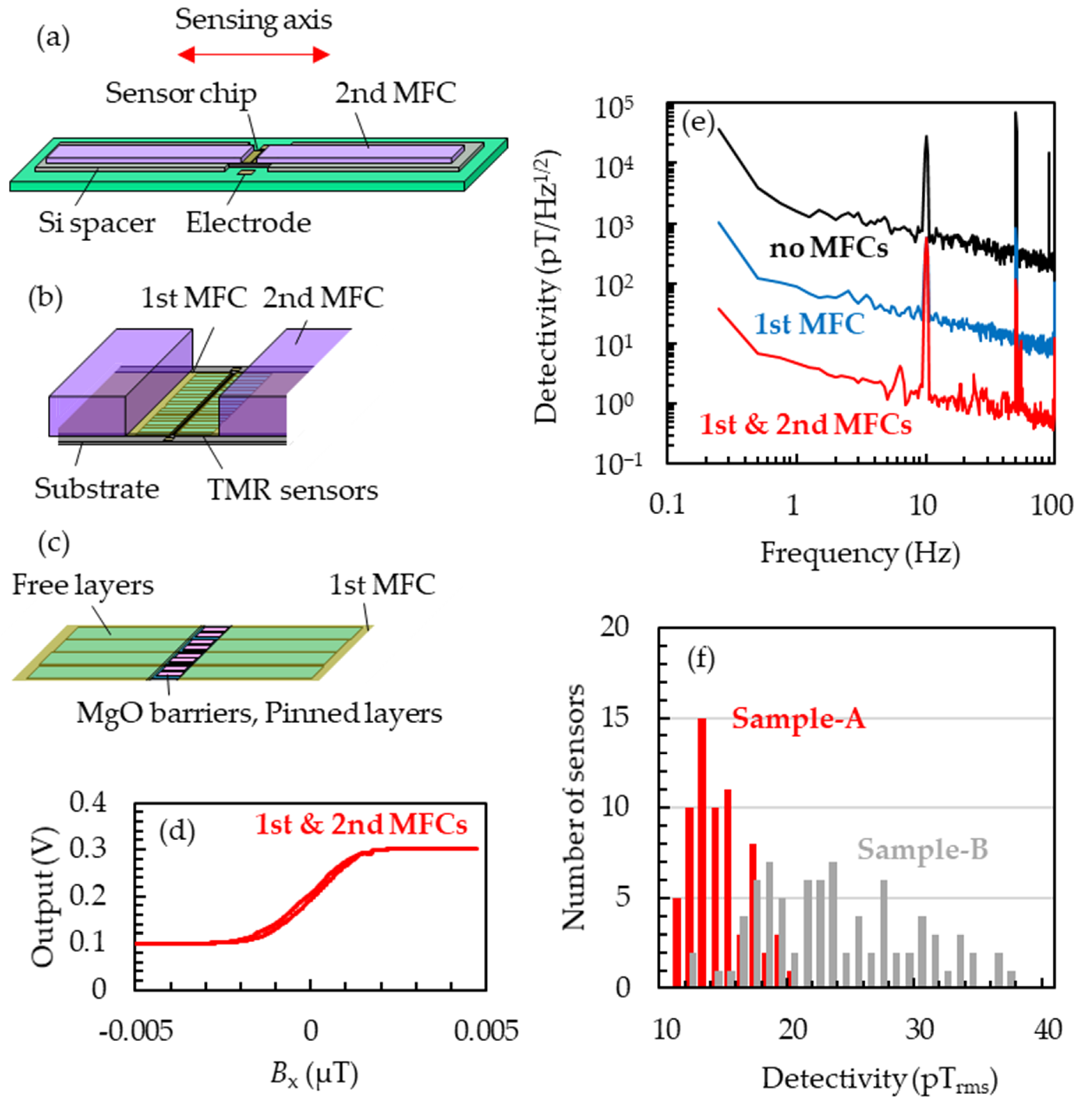
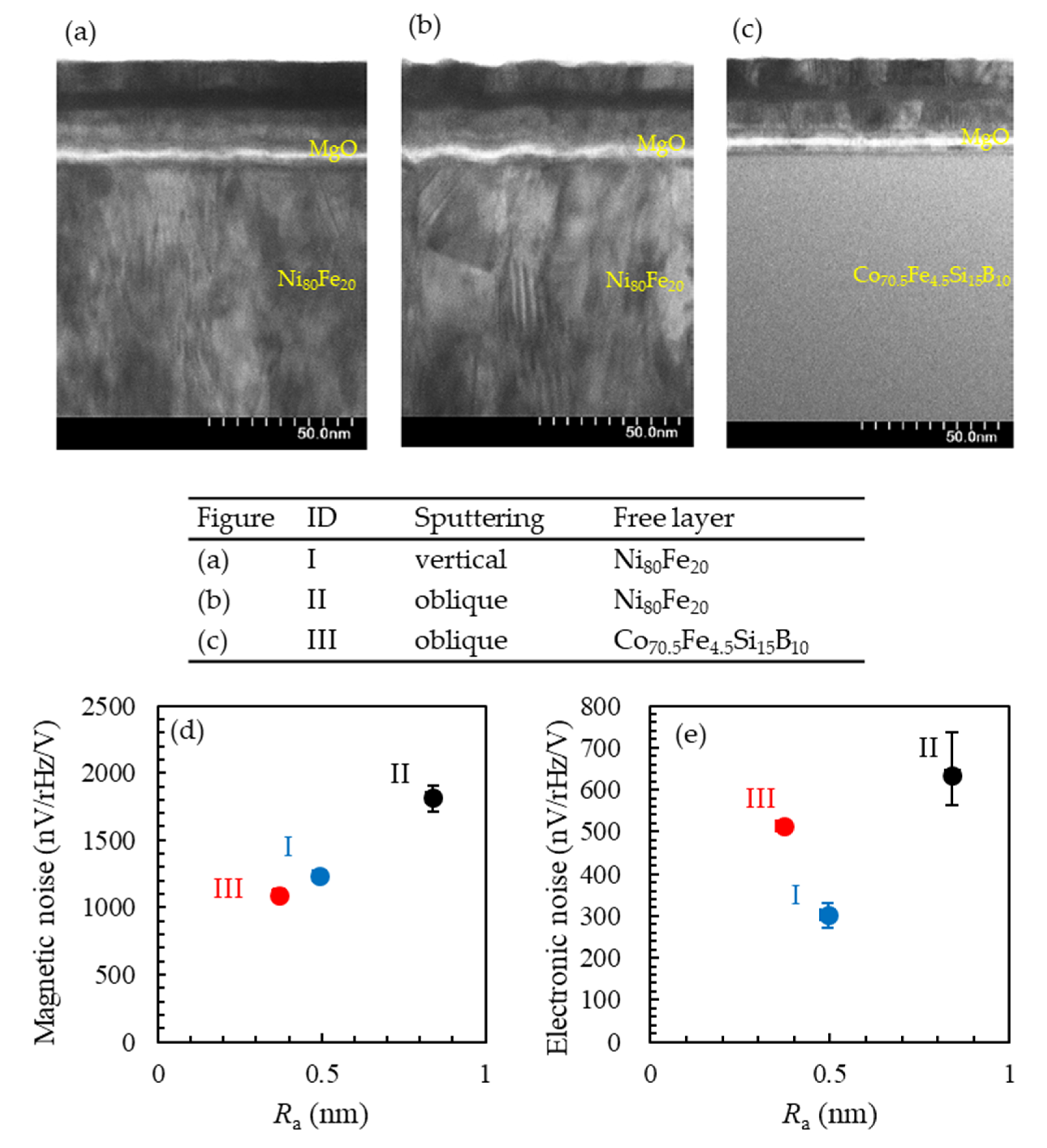
3.1. TMR Sensors
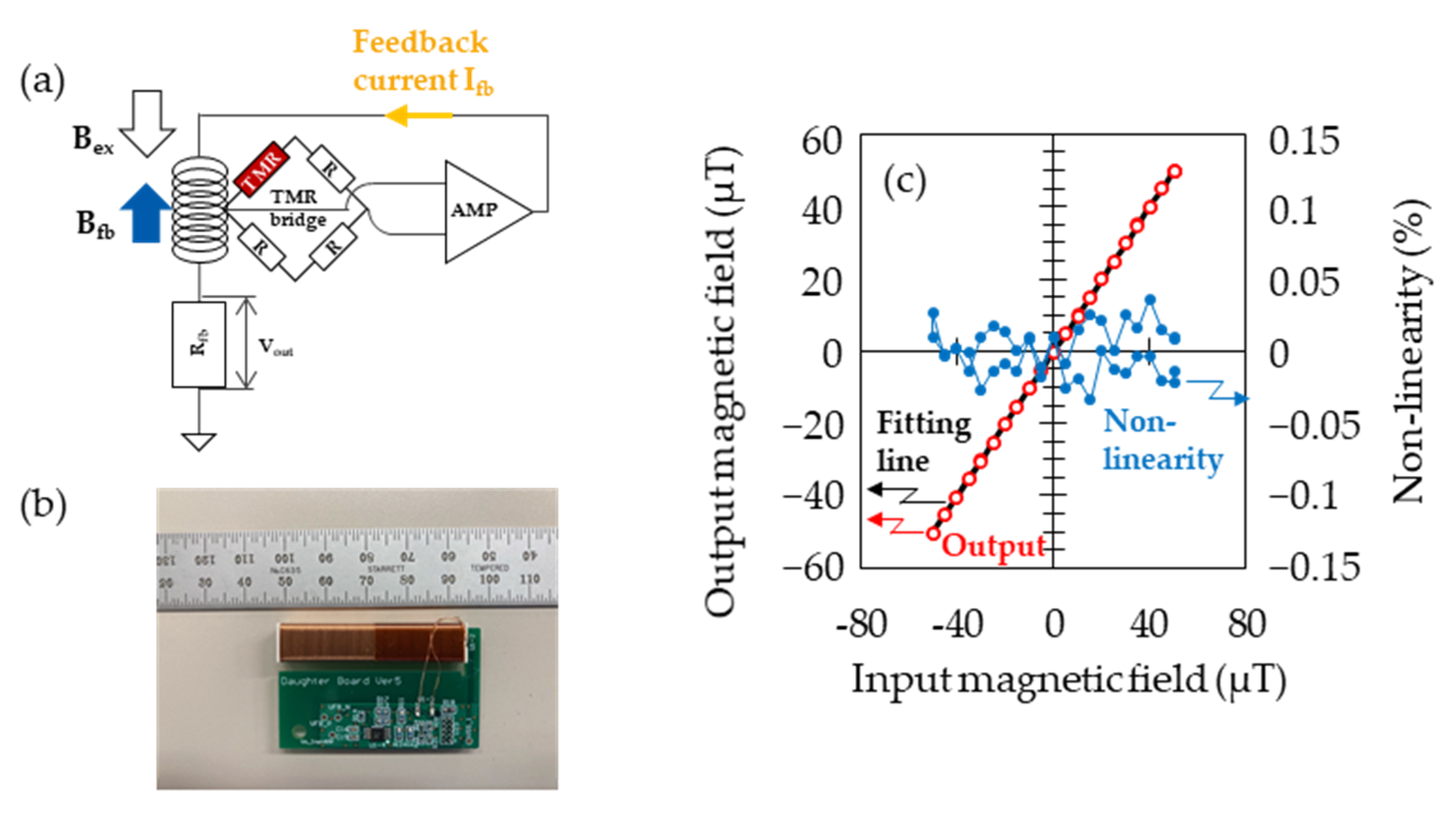
3.2. Closed-Loop Systems
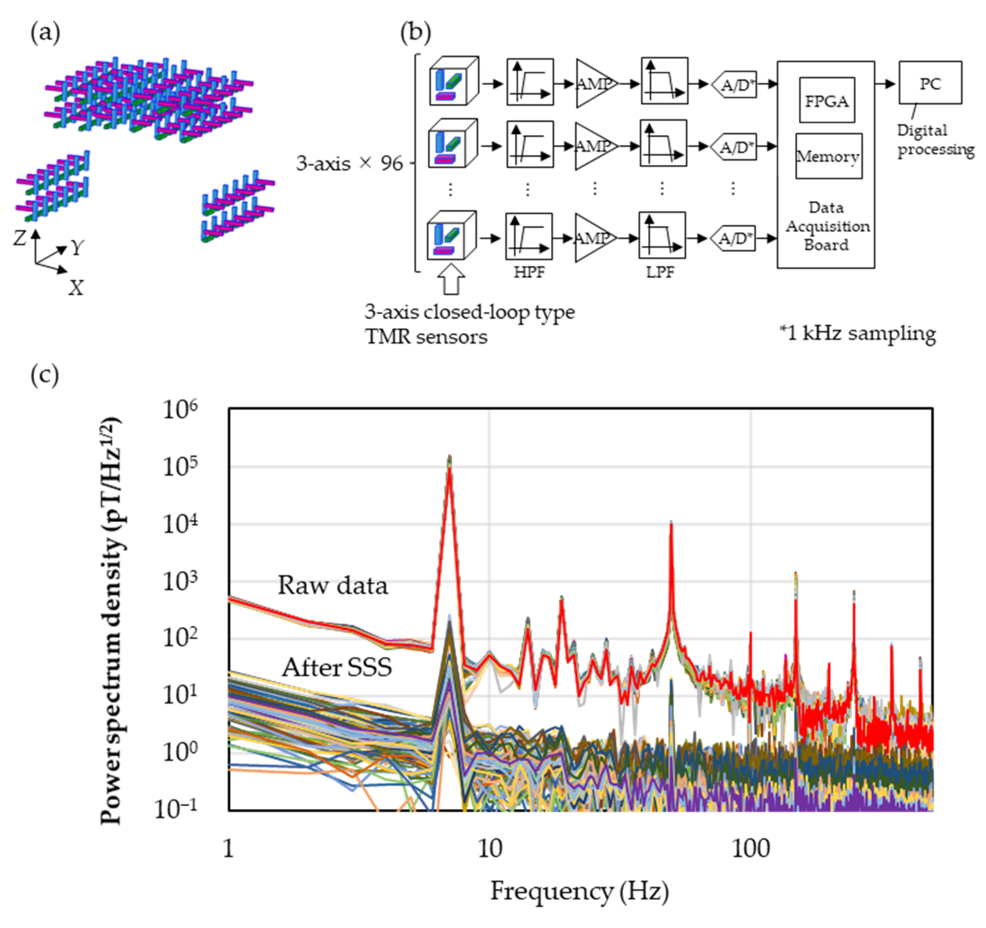
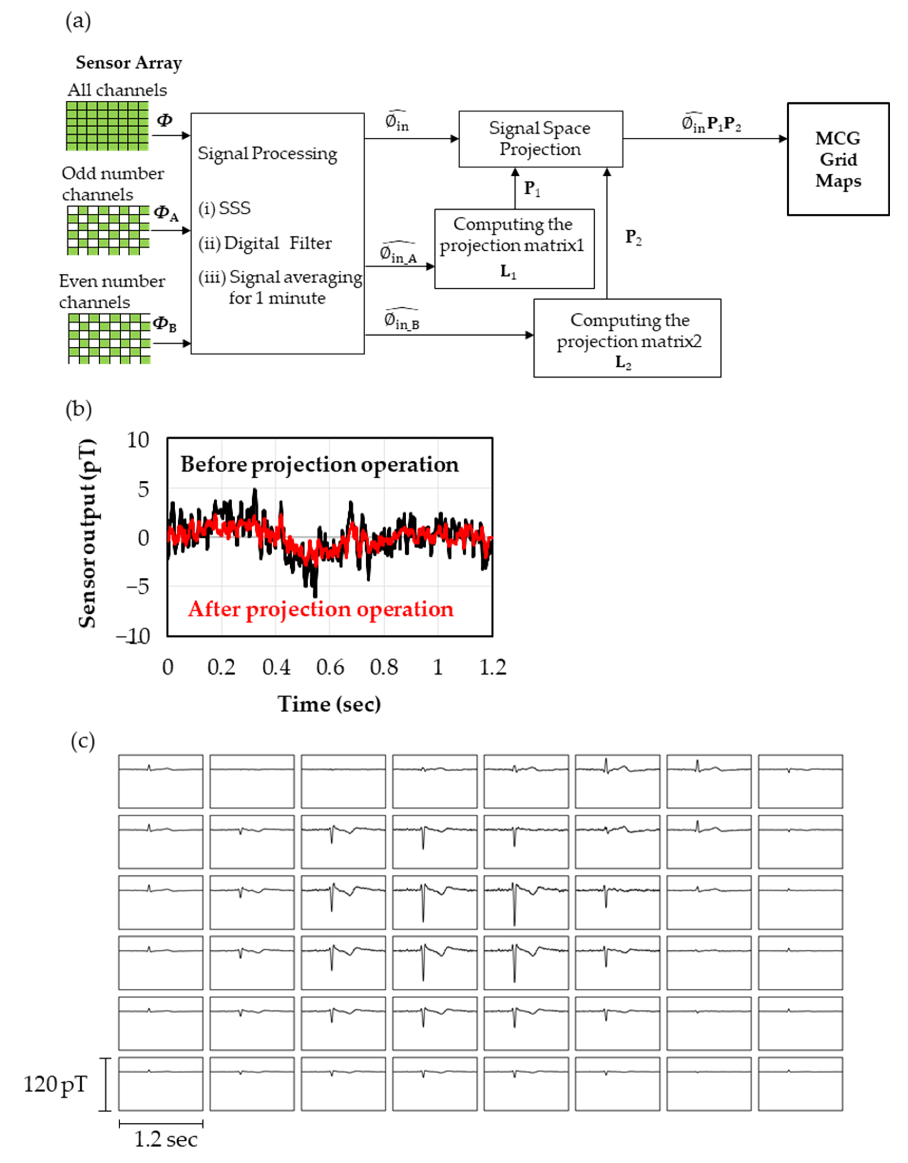
3.3. SSS
3.4. Projection operation
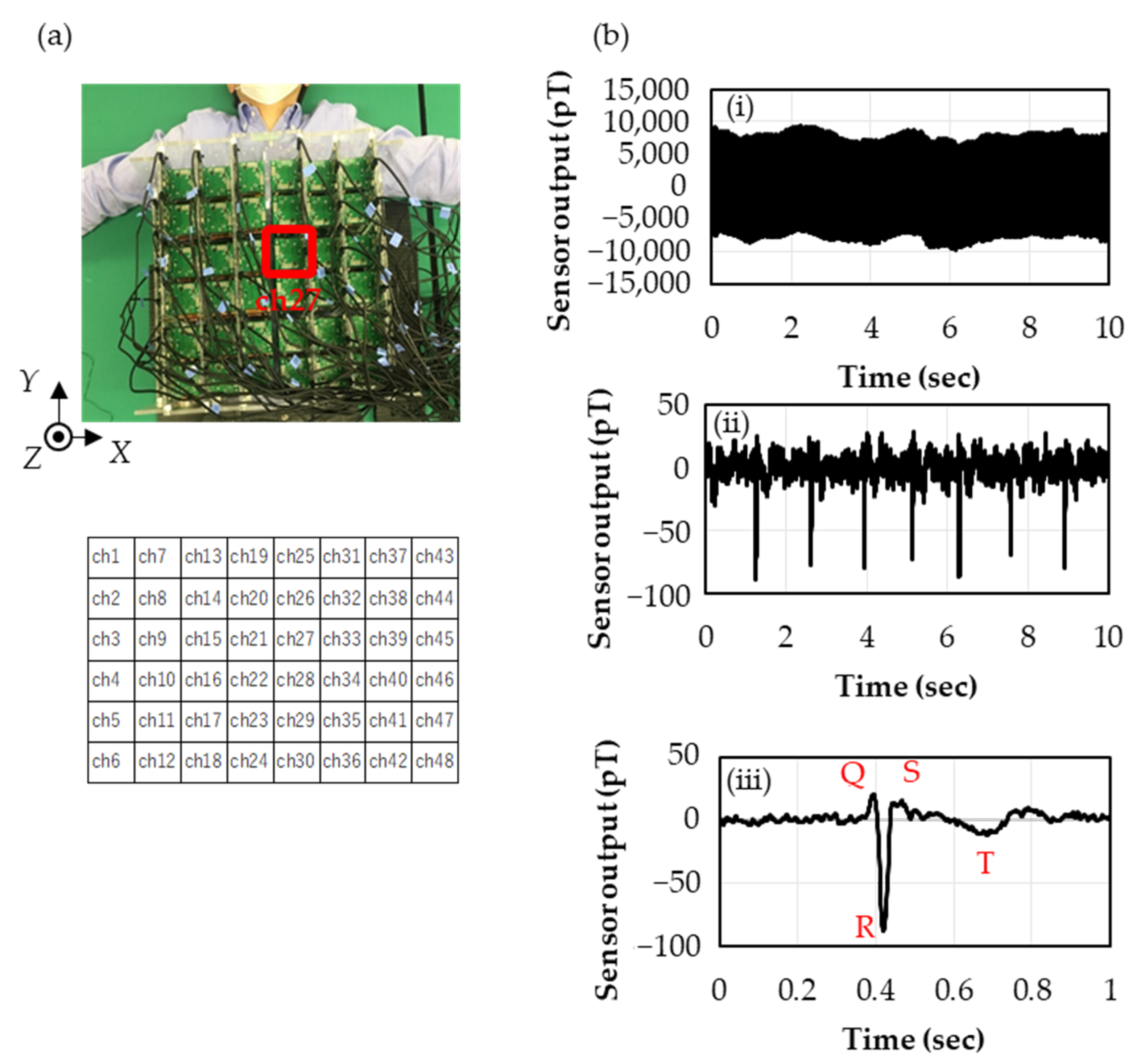
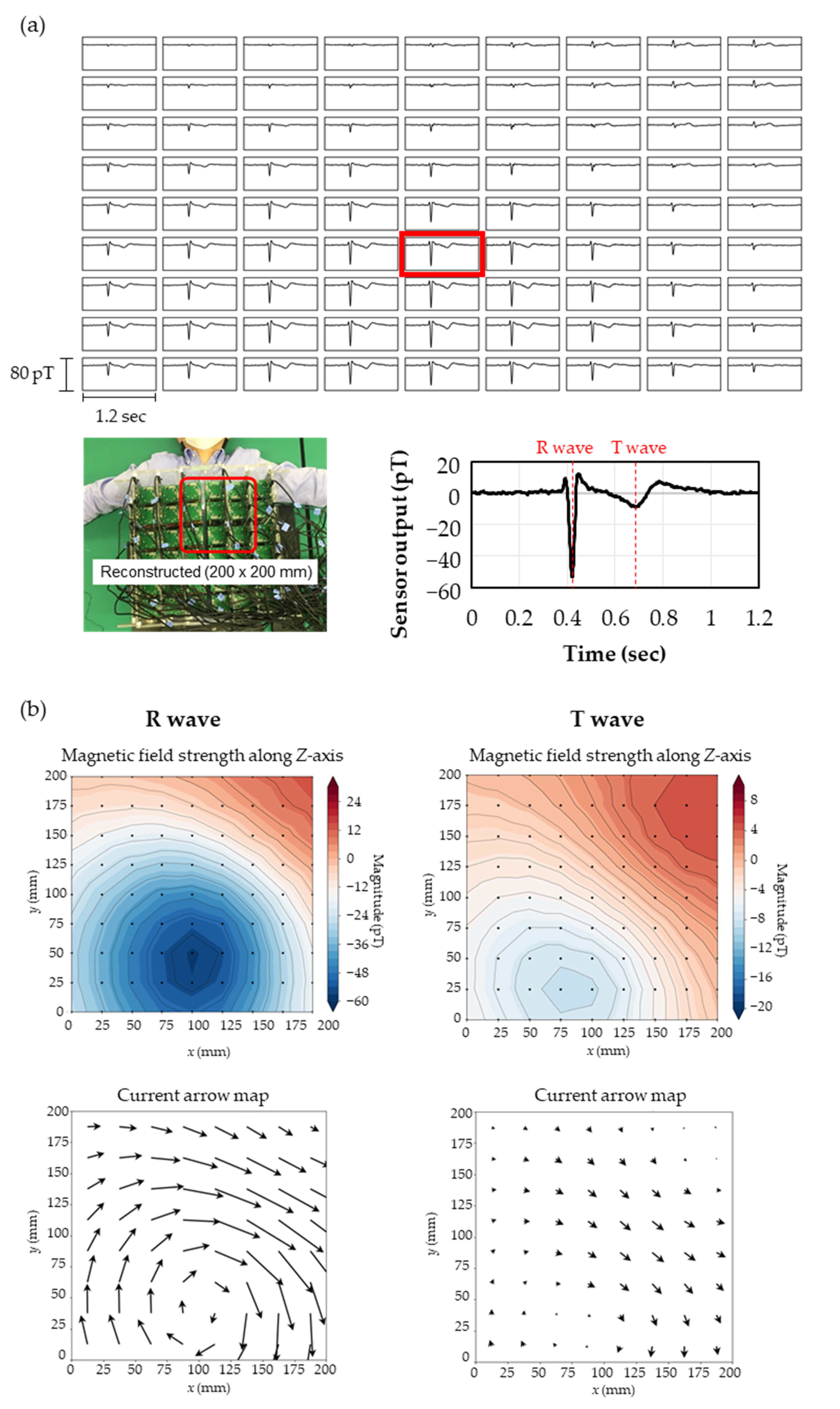
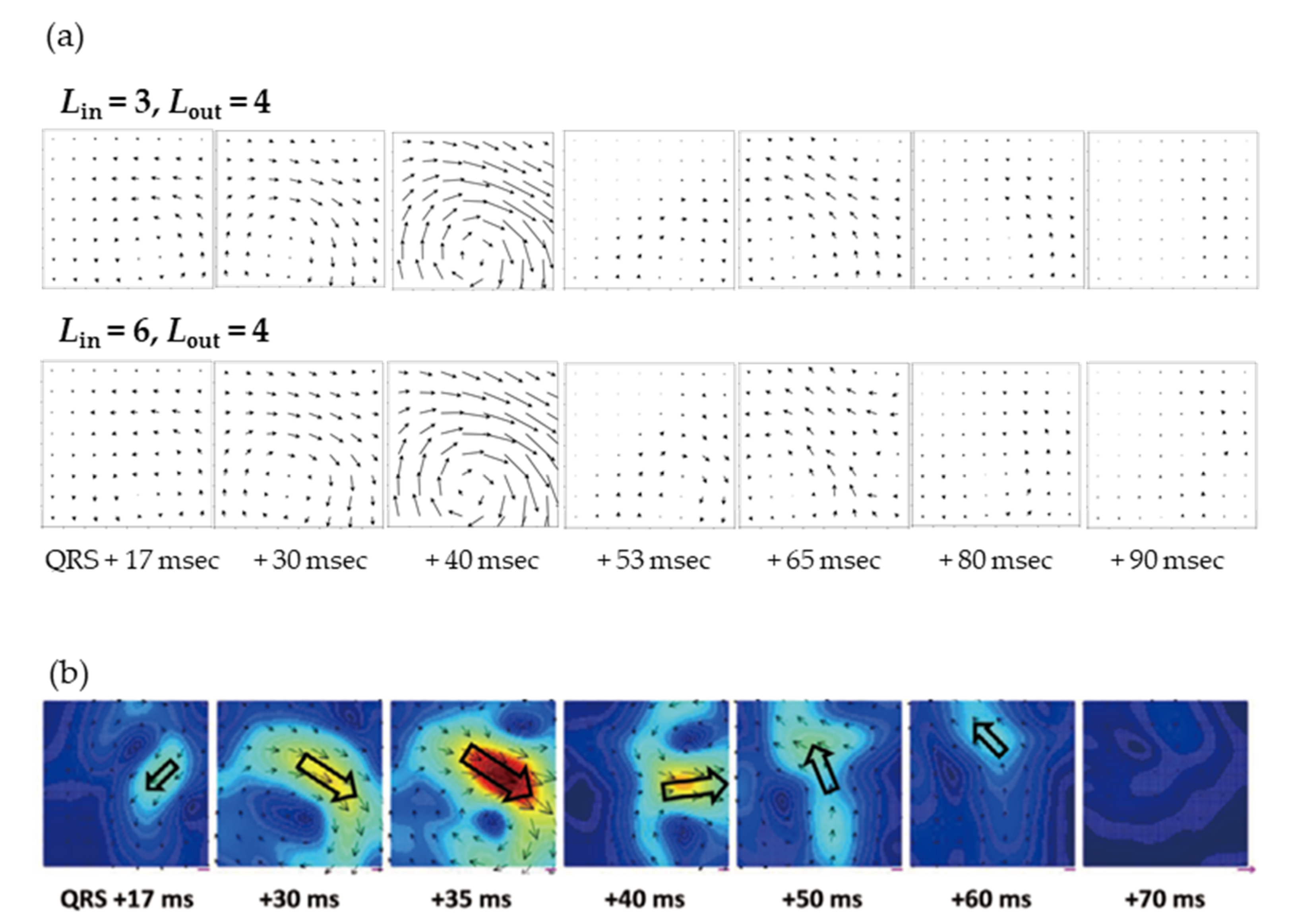
3.5. Preparing the Magnetocardiogram
4. Discussion
4.1. TMR Sensors
4.2. Environmental Noise
4.3. Sensor Noise
5. Conclusions
Author Contributions
Funding
Institutional Review Board Statement
Informed Consent Statement
Data Availability Statement
Acknowledgments
Conflicts of Interest
Appendix A


References
- Fenici, R.; Brisinda, D.; Meloni, M. Clinical application ofmagnetocardiography. Expert Rev. Mol. Diagn. 2005, 5, 291–313. [Google Scholar] [CrossRef]
- Park, J.-W.; Hill, P.M.; Chung, N.; Hugenholtz, P.G.; Jung, F. Magnetocardiography Predicts Coronary Artery Disease in Patients with Acute Chest Pain. Ann. Noninvasive Electrophysiol. 2005, 10, 312–323. [Google Scholar] [CrossRef] [PubMed]
- Hailer, B. The Value of MCG in PTS with and Without Relevant Stenoses of the Coronary Arteries Using an Unshielded System. PACE 2005, 28, 8–16. [Google Scholar] [CrossRef] [PubMed]
- Hailer, B.; Leeuwen, P.V.; Chaikovsky, I.; Auth-Eisernitz, S.; Schäfer, H.; Grönemeyer, D. The Value ofmagnetocardiography in the Course of Coronary Intervention. Ann. Noninvasive Electrophysiol. 2005, 10, 188–196. [Google Scholar] [CrossRef]
- On, K.; Watanabe, S.; Yamada, S.; Takeyasu, N.; Nakagawa, Y.; Nishina, H.; Morimoto, T.; Aihara, H.; Kimura, T.; Sato, Y.; et al. Integral Value of JT Interval inmagnetocardiography in Sensitive to Coronary Stenosis and Improves Soon After Coronary Revascularization. Circ. J. 2007, 71, 1586–1592. [Google Scholar] [CrossRef] [Green Version]
- Zhao, C.; Chen, Y.; Zhao, D.; Wang, J.; Chen, Q. Comparison betweenmagnetocardiography and myocardial perfusion imaging in the diagnosis of myocardial ischemia in patients with coronary artery disease. Int. J. Clin. Exp. Med. 2019, 12, 13127–13134. [Google Scholar]
- Wu, Y.-W.; Lin, L.-C.; Tseng, W.-K.; Liu, Y.-B.; Kao, H.-L.; Lin, M.-S.; Huang, H.-C.; Wang, S.-Y.; Horng, H.-E.; Yang, H.-C.; et al. QTc Heterogeneity in Restmagnetocardiography in Sensitive to Detet Coronary Artery Disease: In Comparison with Stress Myocardial Perfusion Imaging. Acta Cardiol. Sin. 2014, 30, 445–454. [Google Scholar]
- Joung, B.; Kim, K.; Lee, Y.-H.; Kwon, H.; Lim, H.K.; Kim, T.-U.; Ko, Y.-G.; Lee, M.; Chung, N.; Kim, S. Magnetic Dispersion of the Later Repolarization in Brugada Syndrome. Circ. J. 2008, 72, 94–101. [Google Scholar] [CrossRef] [Green Version]
- Kawakami, S.; Takaki, H.; Hashimoto, S.; Kimura, Y.; Nakashima, T.; Aiba, T.; Kusano, K.F.; Kamakura, S.; Yasuda, S.; Sugimachi, M. Utility of High-Resolutionmagnetocardiography to Predict Later Cardiac Events in Noniscemic Cardiomyopathy Patients With Normal QRS Duration. Circ. J. 2017, 81, 44–51. [Google Scholar] [CrossRef] [Green Version]
- Kimura, Y.; Takaki, H.; Inoue, Y.Y.; Oguchi, Y.; Nagayama, T.; Nakashima, T.; Kawakami, S.; Nagase, S.; Noda, T.; Aiba, T.; et al. Isolated Late Activation Detected bymagnetocardiography Predicts Future Lethal Ventricular Arrhythmic Events in Patients With Arrhythmogenic Right Ventricular Cardiomyopathy. Circ. J. 2018, 82, 78–86. [Google Scholar] [CrossRef] [Green Version]
- Hailer, B.; Leeuwen, P.-V. Prediction of malignant arrhythmias after myocardial infarction on the basis of MCG. In Proceedings of the 12th International Conference on Biomagnetism, Espoo, Finland, 13–17 August 2000; pp. 504–507. [Google Scholar]
- Ando, Y.; Nishikawa, T.; Fujiwara, K.; Oogane, M.; Kato, D.; Naganuma, H. Present and perspective of bio-magnetic measurement using ferromagnetic tunnel junctions. Jpn. Soc. Med. Biol. Eng. 2014, 52, OS-33–OS-34. [Google Scholar]
- Boto, E.; Holmes, N.; Leggett, J.; Roberts, G.; Shah, V.; Meyer, S.S.; Muñoz, L.D.; Mullinger, K.; Tierney, T.M.; Bestmann, S.; et al. Moving magnetoencephalography towards real-world applications with a wearable system. Nature 2018, 555, 657–661. [Google Scholar] [CrossRef] [Green Version]
- Knappe, S.; Sander, T.; Trahms, L. Optically pumped magnetometers for MEG. In Magnetoencephalography, 2nd ed.; Supek, S., Aine, C.J., Eds.; Springer Nature: Cham, Switzerland, 2019; pp. 1301–1312. [Google Scholar]
- Arai, K.; Kuwahata, A.; Nishitaki, D.; Fujisaki, I.; Matsuki, R.; Xin, Z.; Nishio, Y.; Cao, X.; Hatano, Y.; Onoda, S.; et al. Millimetre-scale magnetocardiography of licing rats using a solid-state quantum sensor. arXiv 2021, arXiv:2105.11676. [Google Scholar]
- Hayashi, K.; Matsuzaki, Y.; Ashida, T.; Onoda, S.; Abe, H.; Ohshima, T.; Hatano, M.; Taniguchi, T.; Morishita, H.; Fujiwara, M.; et al. Experimental and Theoretical Analysis of Noise Strength and Environmental Correlation Time for Ensembles of Nitrogen-Vacancy Centers in Diamond. J. Phys. Soc. Jpn. 2020, 89, 054708. [Google Scholar] [CrossRef]
- Kanno, A.; Nakasato, N.; Oogane, M.; Fujiwara, K.; Nakano, T.; Arimoto, T.; Matsuzaki, H.; Ando, Y. Scalp attached tangential magnetoencephalography using tunnel magneto-resistive sensors. Sci. Rep. 2022, 12, 6106. [Google Scholar] [CrossRef] [PubMed]
- Shirai, Y.; Hirao, K.; Shibuya, T.; Okuwa, S.; Hasegawa, Y.; Adachi, Y.; Sekihara, K.; Kawabata, S. Magnetocardiography Using a Magnetoresistive Sensor Array. Int. Heart J. 2019, 60, 50–54. [Google Scholar] [CrossRef] [Green Version]
- Adachi, Y.; Oyama, D.; Terazono, Y.; Hayashi, T.; Shibuya, T.; Kawabata, S. Calibration of Room Temperature Magnetic Sensor Array for Biomagnetic Measurement. IEEE Trans. Magn. 2019, 55, 1000506. [Google Scholar] [CrossRef]
- Zhao, W.; Tao, X.; Ye, C.; Tao, Y. Tunnel Magnetoresistance Sensor with AC Modulation and Impedance Compensation for Ultra-Weak Magnetic Field Measurement. Sensors 2022, 22, 1021. [Google Scholar] [CrossRef] [PubMed]
- Davies, J.E.; Watts, J.D.; Novotny, J.; Huang, D.; Eames, P.G. Magnetoresistive sensor detectivity: A comparative analysis. App. Phys. Lett. 2021, 118, 062401. [Google Scholar] [CrossRef]
- Watanabe, S.; Yamada, S. Magnetocardiography in Early Detection of Electromagnetic Abnormality in Ischemic Heart Disease. J. Arrhythmia 2008, 24, 4. [Google Scholar] [CrossRef]
- Oogane, M.; Fujiwara, K.; Kanno, A.; Nakano, T.; Wagatsuma, H.; Arimoto, T.; Mizukami, S.; Kumagai, S.; Matsuzaki, H.; Nakasato, N.; et al. Sub-pT magnetic field detection by tunnel magneto-resistive sensors. Appl. Phys. Express 2021, 14, 123002. [Google Scholar] [CrossRef]
- Fujiwara, K.; Oogane, M.; Nishikawa, T.L.; Naganuma, H.; Ando, Y. Fabrication of magnetic tunnel junctions with a bottom synthetic antiferro-coupled free layers for high sensitive magnetic field sensor device. J. Appl. Phys. 2012, 111, 07C710. [Google Scholar] [CrossRef]
- Fujiwara, K.; Oogane, M.; Kanno, A.; Imada, M.; Jono, J.; Terauchi, T.L.; Okuno, T.; Aritomi, Y.; Morikawa, M.; Tsuchida, M.; et al. Magnetocardiography and magnetoencephalography measurements at room temperature using tunnel magnetoresistance. Appl. Phys. Express 2018, 11, 023001. [Google Scholar] [CrossRef]
- Kato, D.; Oogane, M.; Fujiwara, K.; Nishikawa, T.; Naganuma, H.; Ando, Y. Fabrication of Magnetic Tunnel Junctions with Amorphus CoFeSiB Ferromagnetic Electrode for Magnetic Field Sensor Devices. Appl. Phys. Exp. 2013, 6, 103004. [Google Scholar] [CrossRef]
- Taulu, S.; Kajola, M. Presentation of electromagnetic multichannel data: The signal space separation method. J. Appl. Phys. 2005, 97, 124905. [Google Scholar] [CrossRef] [Green Version]
- Stroink, G.; Meeder, R.J.J.; Elliott, P.; Lant, J.; Gardner, M.J. Arrhythmia Vulnerability Assessment Using Magnetic Field Maps and Body Surface Potential Maps. PACE 1999, 22, 1718–1728. [Google Scholar] [CrossRef]
- Welland, M.E.; Koch, R.H. Spatial location of electron trapping defects on silicon by scanning tunneling microscopy. Appl. Phys. Lett. 1986, 48, 724. [Google Scholar] [CrossRef]
- Egelhoff, W.F., Jr.; Pong, P.W.T.; Unguris, J.; McMichael, R.D.; Nowak, E.R.; Edelstein, A.S.; Burnette, J.E.; Fischer, G.A. Critical challenges for picoTesla magnetic-tunnel-junction sensors. Sens. Actuators A 2009, 115, 217–225. [Google Scholar] [CrossRef]
- Aharoni, A. Demagnetizing factors for rectangular ferromagnetic prisms. J. Appl. Phys. 1998, 83, 3432. [Google Scholar] [CrossRef]


Disclaimer/Publisher’s Note: The statements, opinions and data contained in all publications are solely those of the individual author(s) and contributor(s) and not of MDPI and/or the editor(s). MDPI and/or the editor(s) disclaim responsibility for any injury to people or property resulting from any ideas, methods, instructions or products referred to in the content. |
© 2023 by the authors. Licensee MDPI, Basel, Switzerland. This article is an open access article distributed under the terms and conditions of the Creative Commons Attribution (CC BY) license (https://creativecommons.org/licenses/by/4.0/).
Share and Cite
Kurashima, K.; Kataoka, M.; Nakano, T.; Fujiwara, K.; Kato, S.; Nakamura, T.; Yuzawa, M.; Masuda, M.; Ichimura, K.; Okatake, S.; et al. Development of Magnetocardiograph without Magnetically Shielded Room Using High-Detectivity TMR Sensors. Sensors 2023, 23, 646. https://doi.org/10.3390/s23020646
Kurashima K, Kataoka M, Nakano T, Fujiwara K, Kato S, Nakamura T, Yuzawa M, Masuda M, Ichimura K, Okatake S, et al. Development of Magnetocardiograph without Magnetically Shielded Room Using High-Detectivity TMR Sensors. Sensors. 2023; 23(2):646. https://doi.org/10.3390/s23020646
Chicago/Turabian StyleKurashima, Koshi, Makoto Kataoka, Takafumi Nakano, Kosuke Fujiwara, Seiichi Kato, Takenobu Nakamura, Masaki Yuzawa, Masanori Masuda, Kakeru Ichimura, Shigeki Okatake, and et al. 2023. "Development of Magnetocardiograph without Magnetically Shielded Room Using High-Detectivity TMR Sensors" Sensors 23, no. 2: 646. https://doi.org/10.3390/s23020646