

Upper Limb Position Tracking with a Single Inertial Sensor Using Dead Reckoning Method with Drift Correction Techniques
 ,
,  ,
, 
Abstract
:1. Introduction
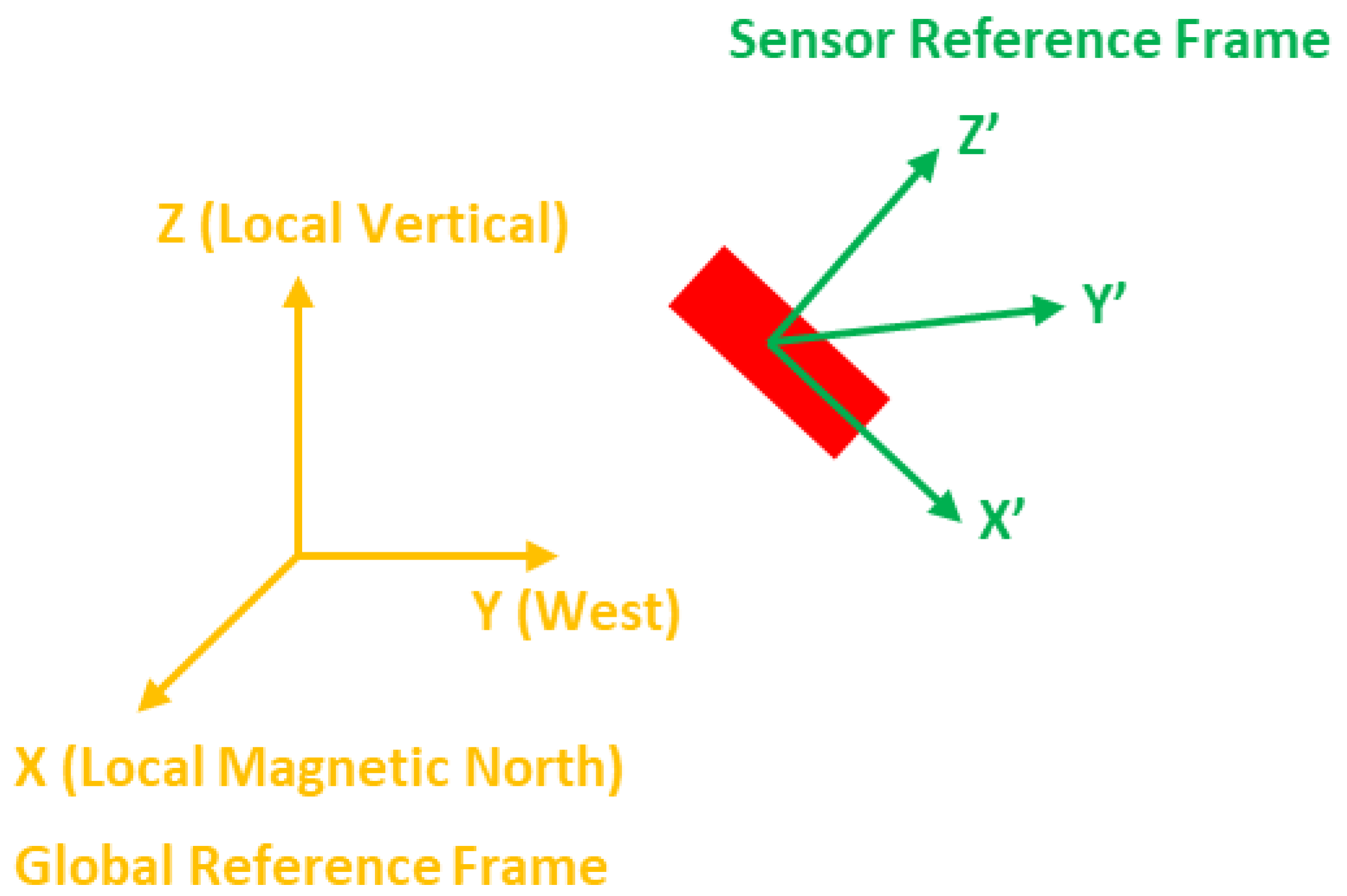
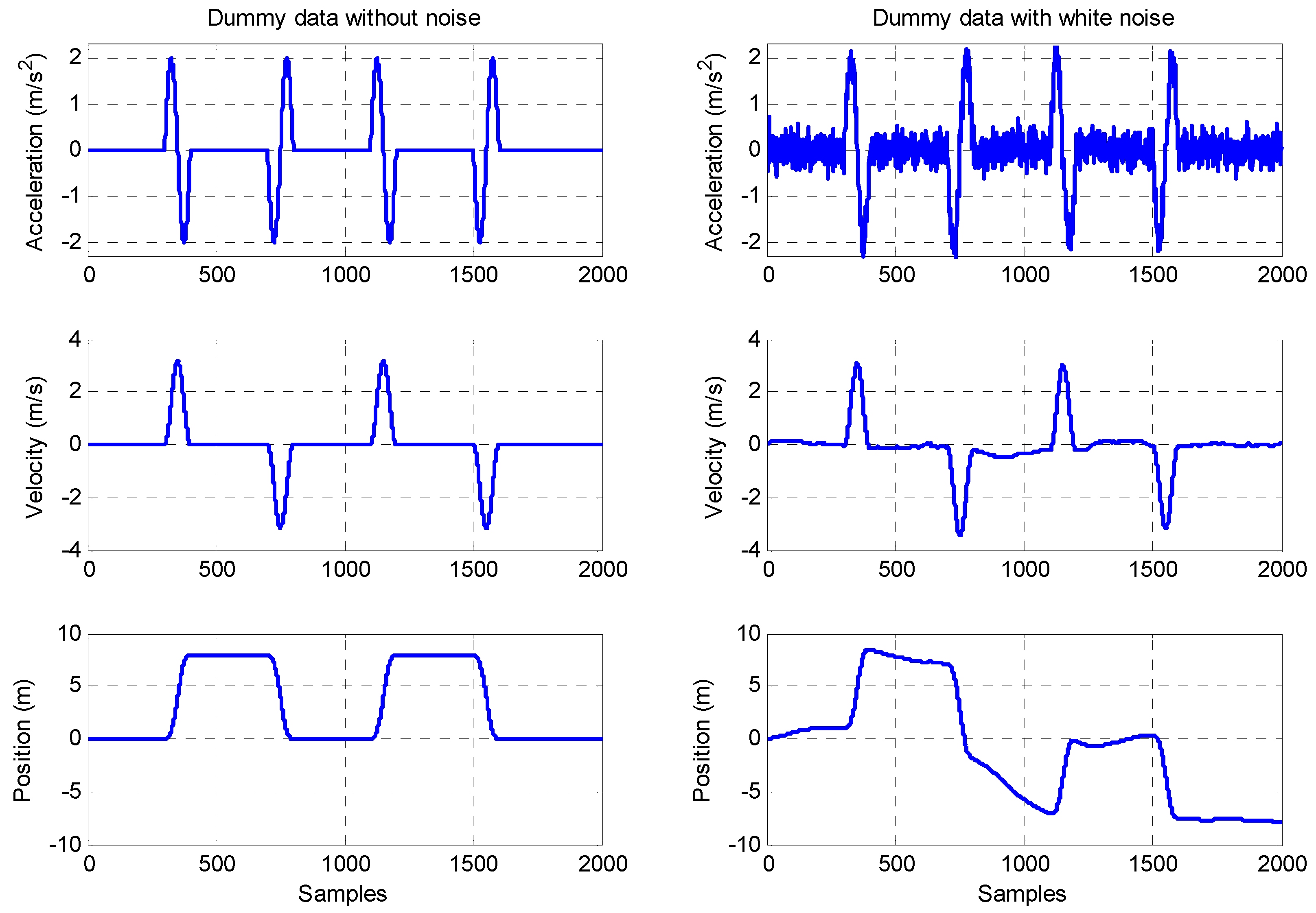
2. DR Method
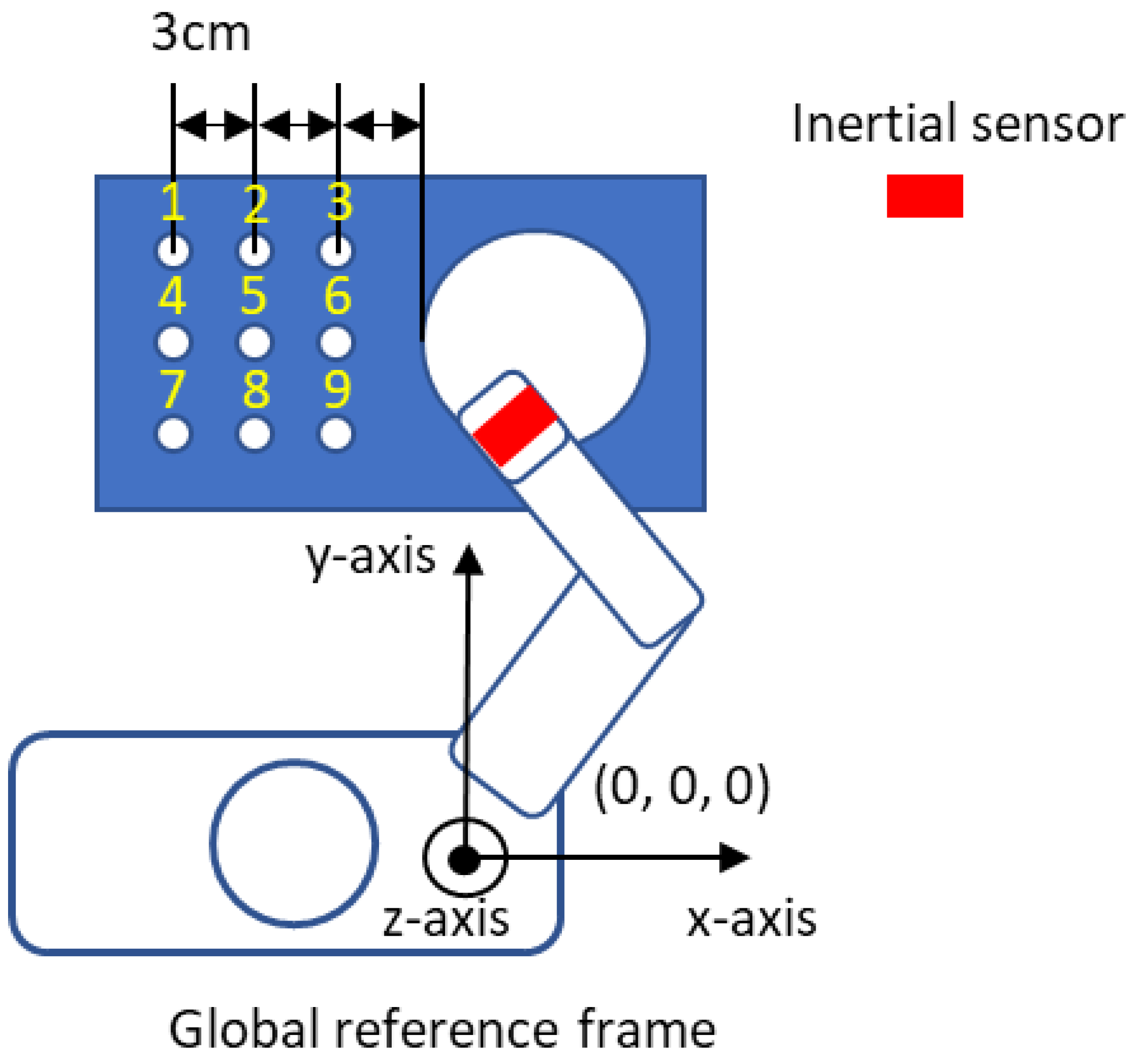
3. Methods
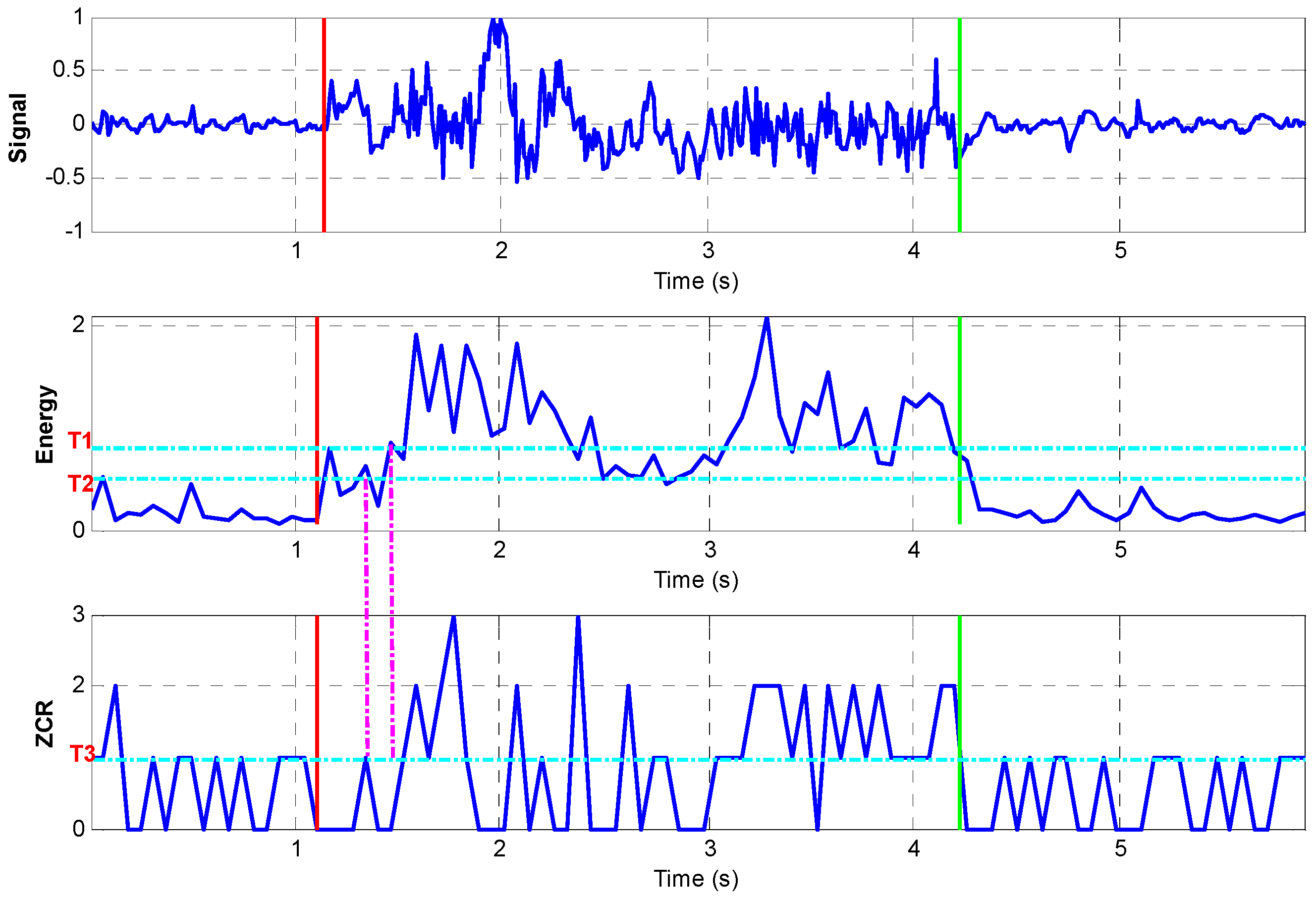
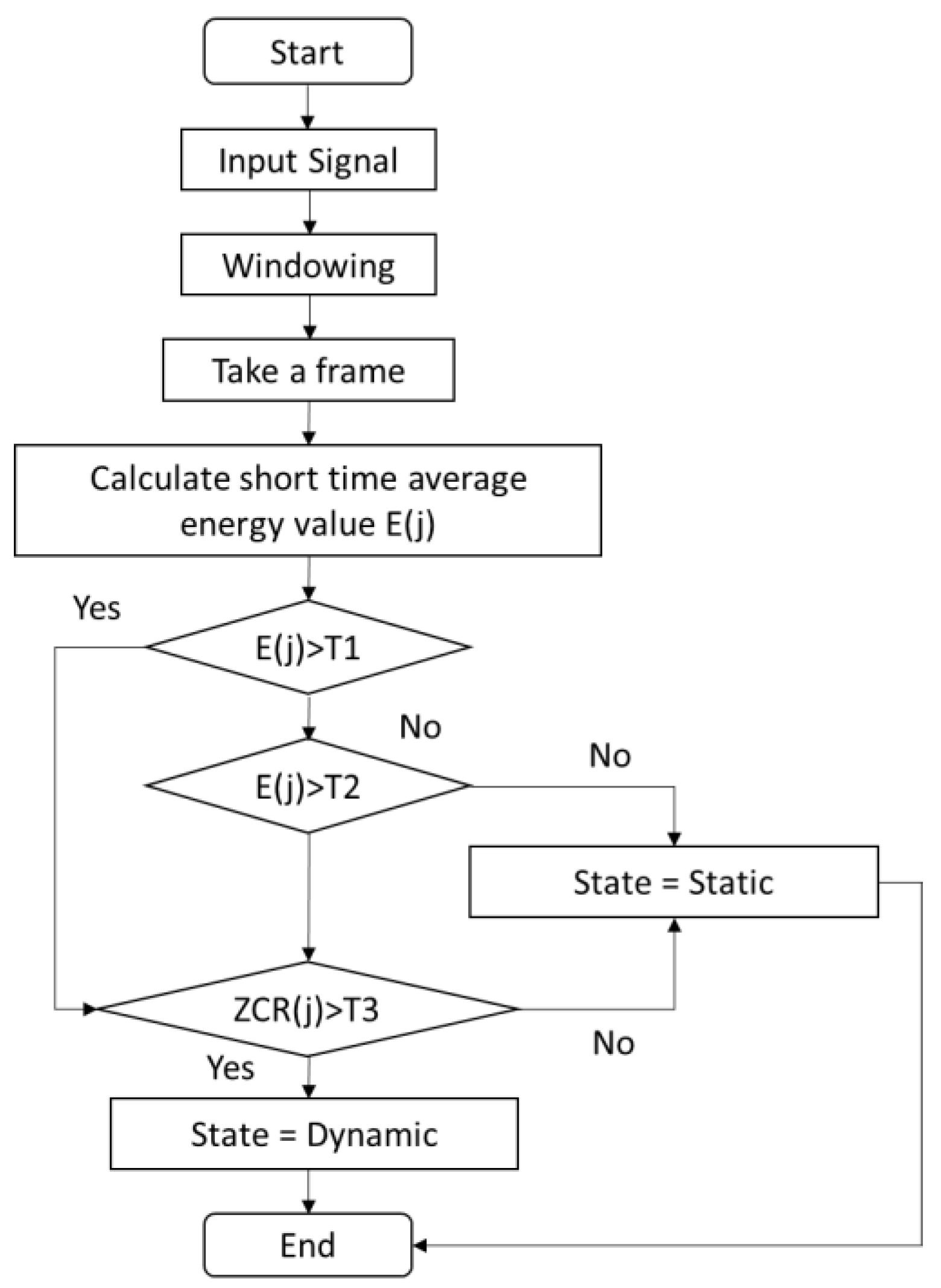
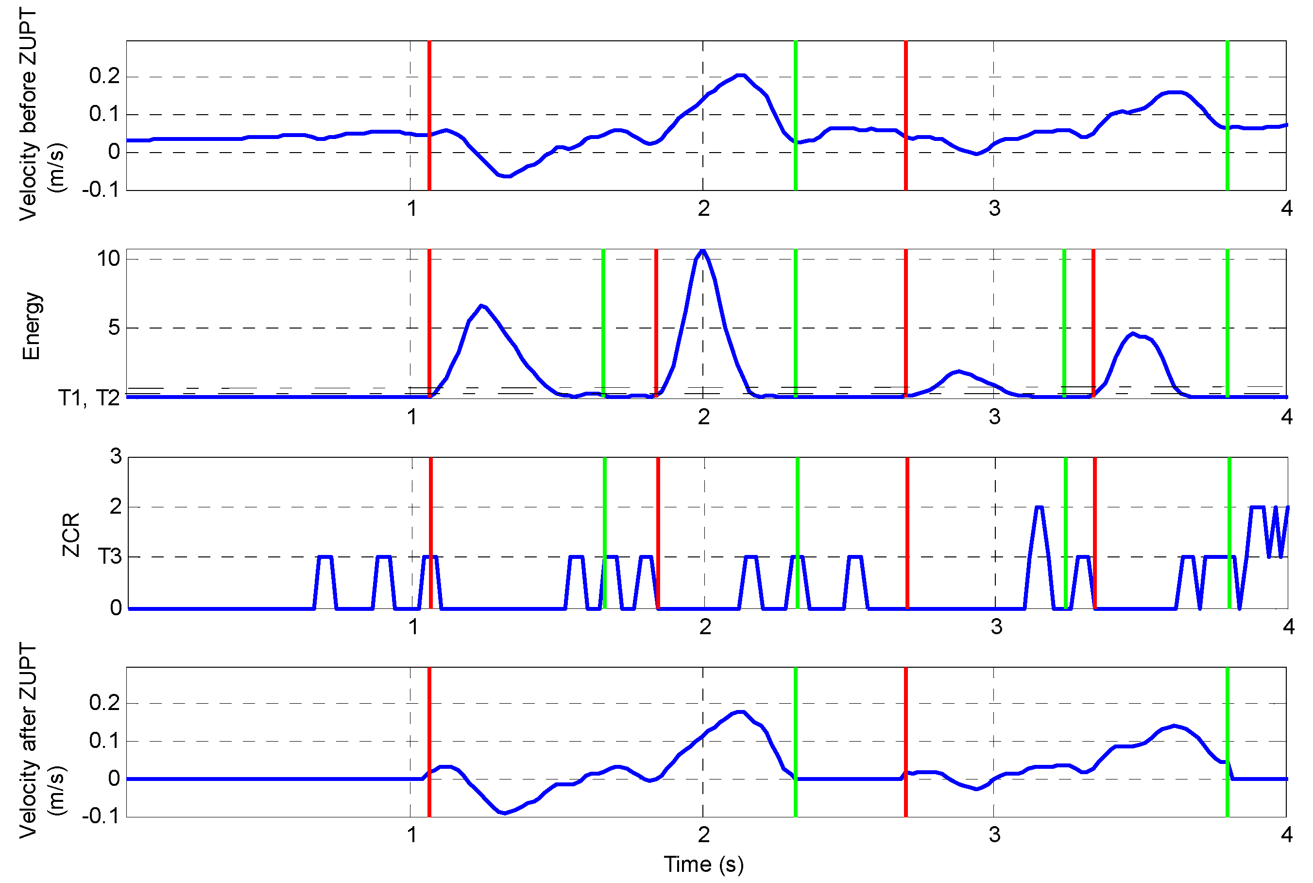
3.1. ZUPT
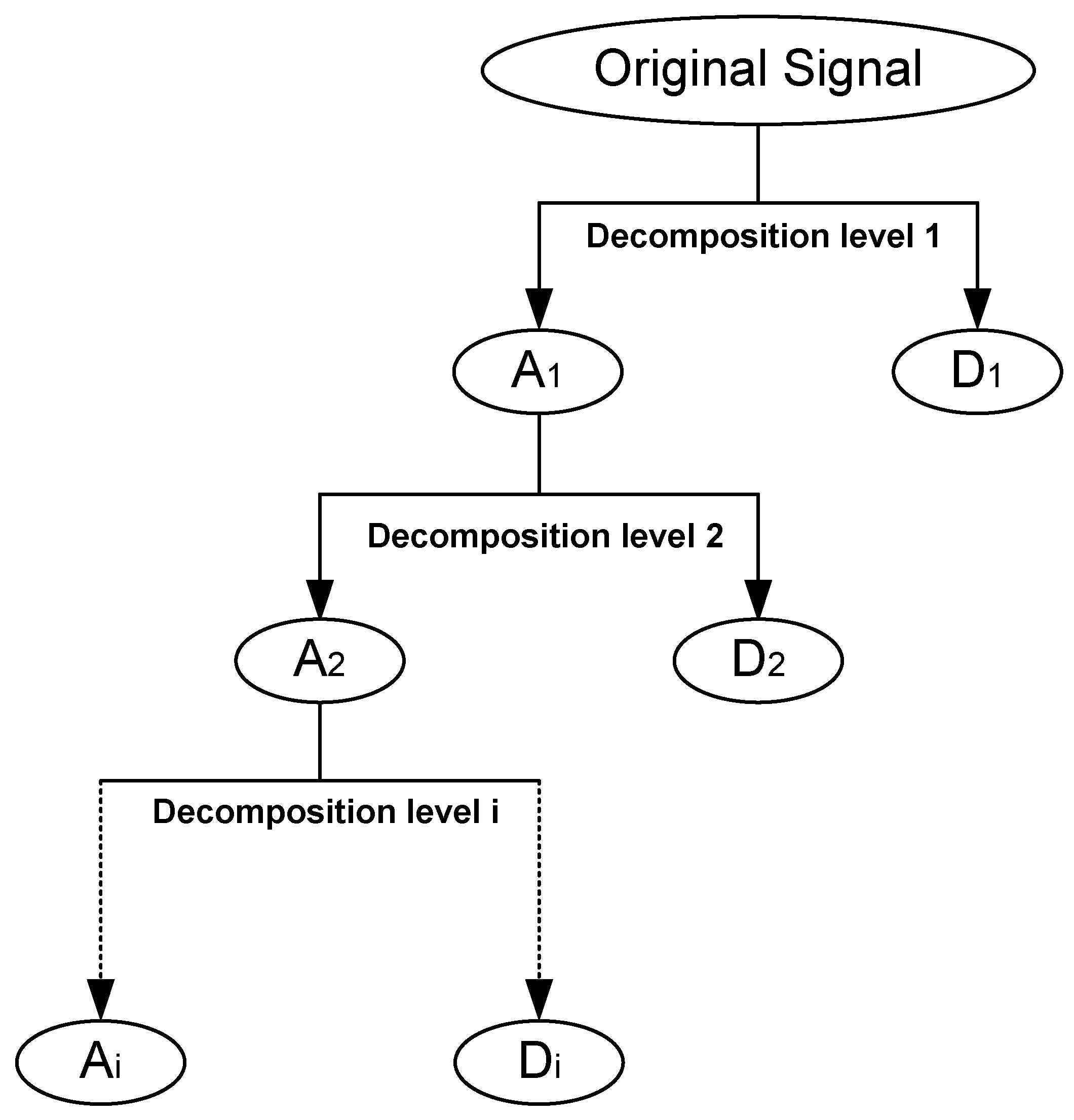
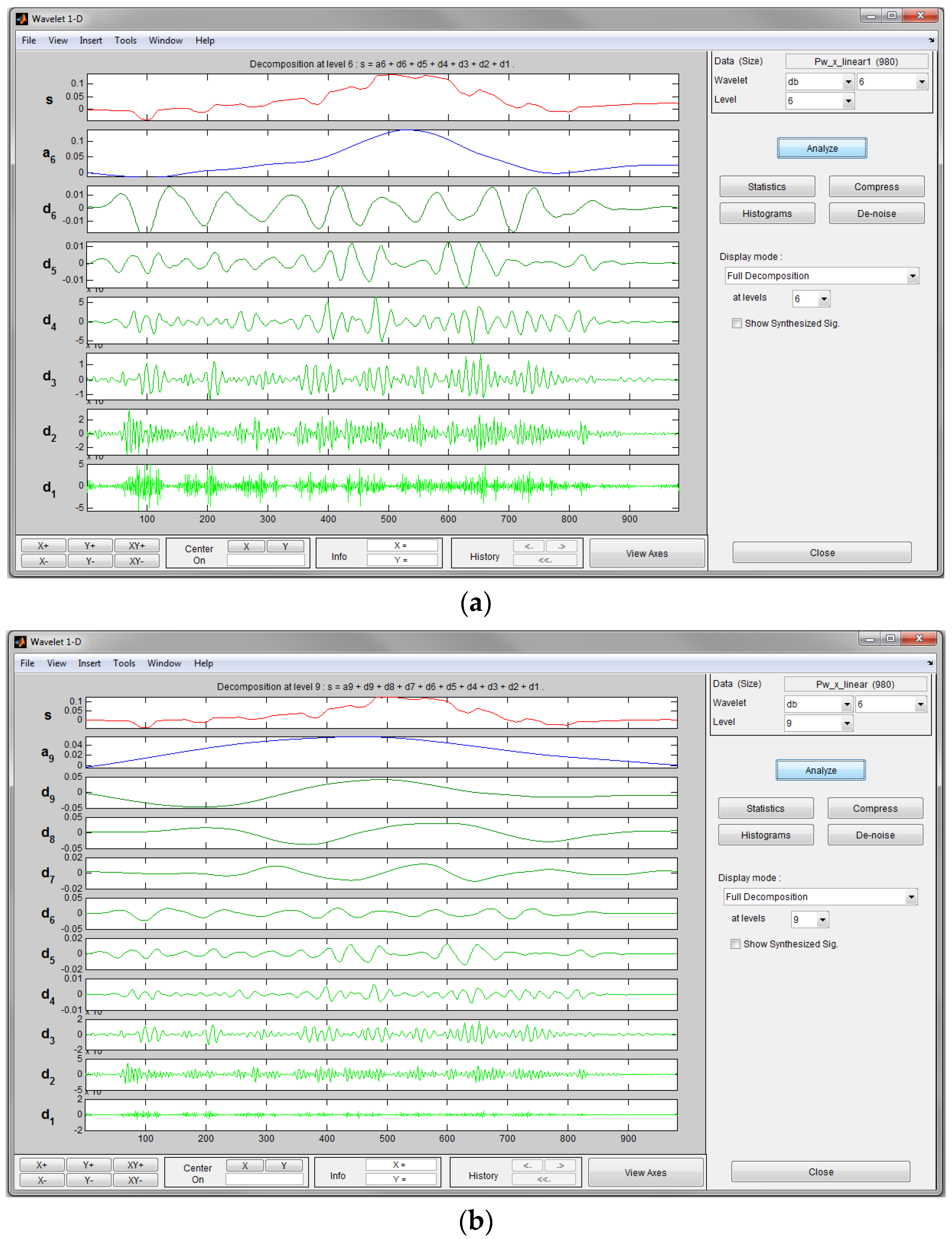
3.2. Wavelet Analysis
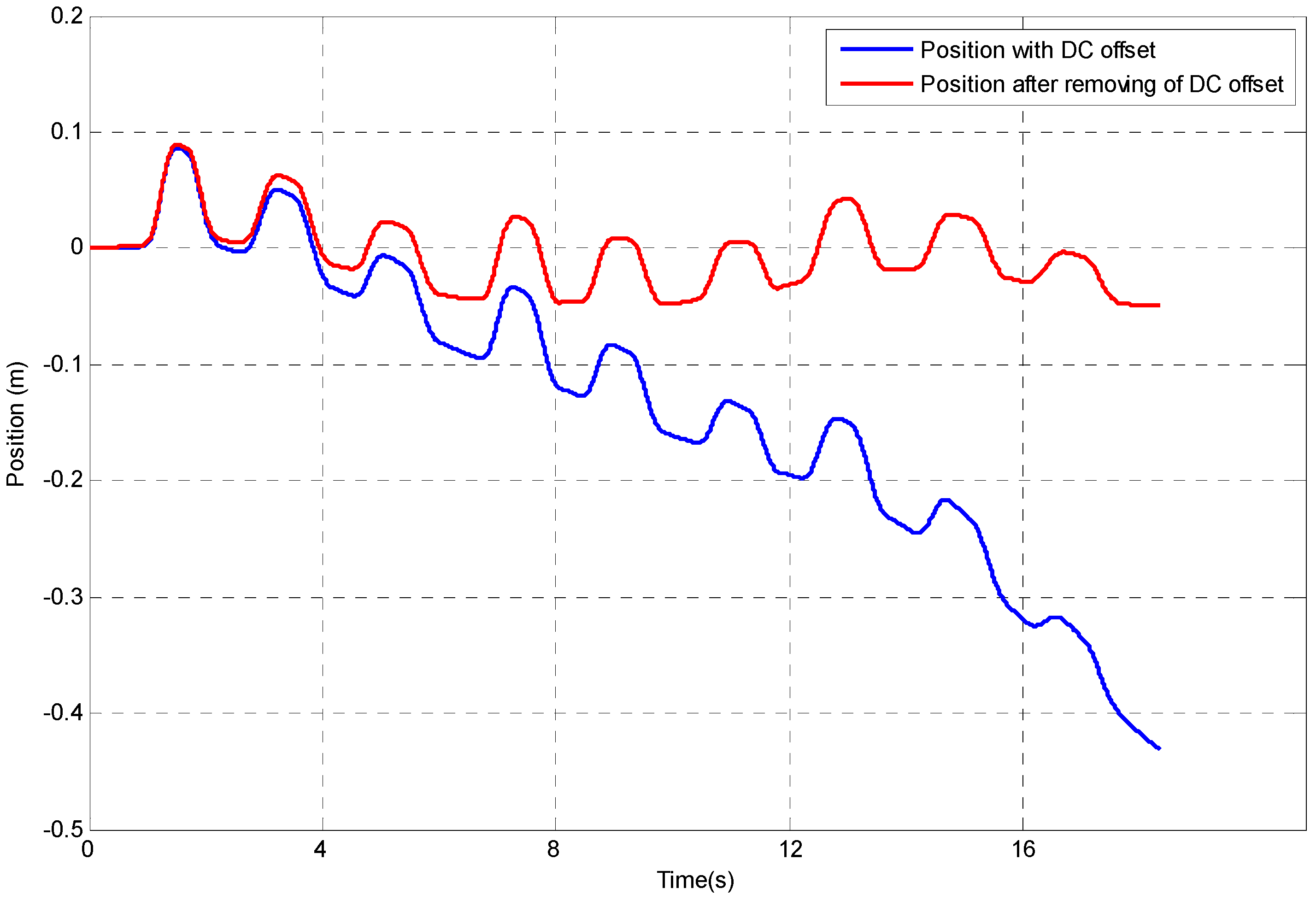
3.3. High-Pass (HP) Filter
4. Results and Discussion
4.1. Results Using ZUPT
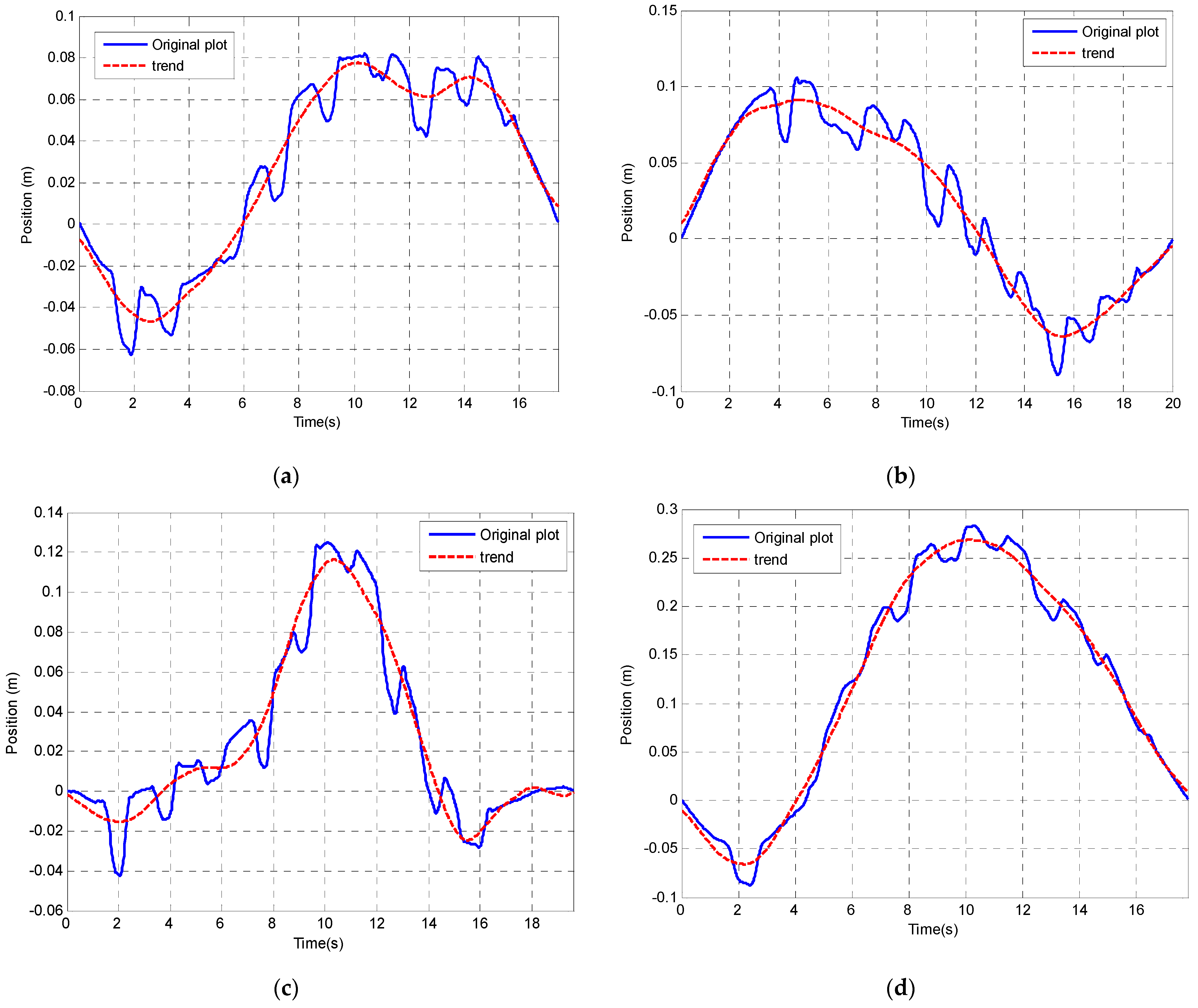
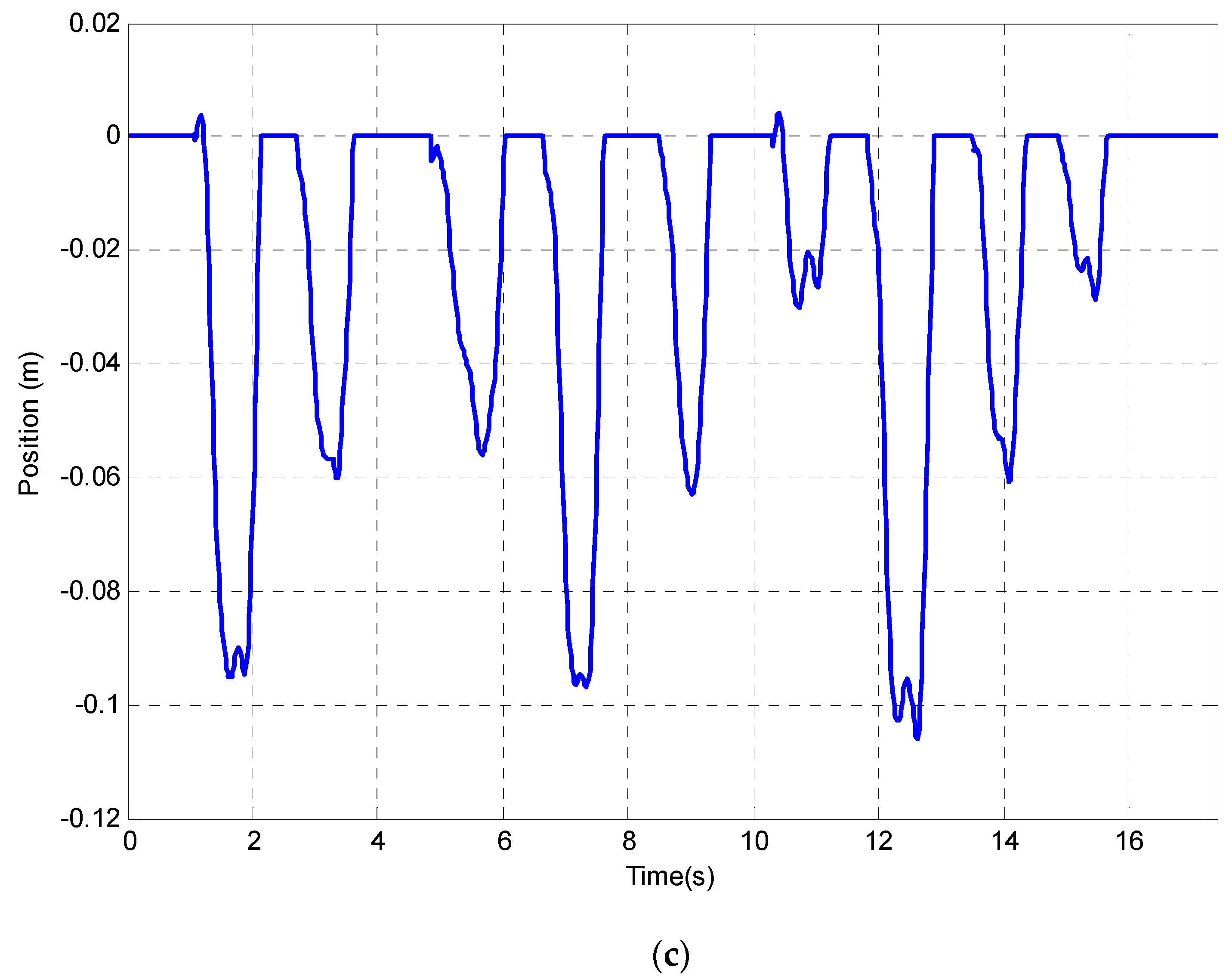
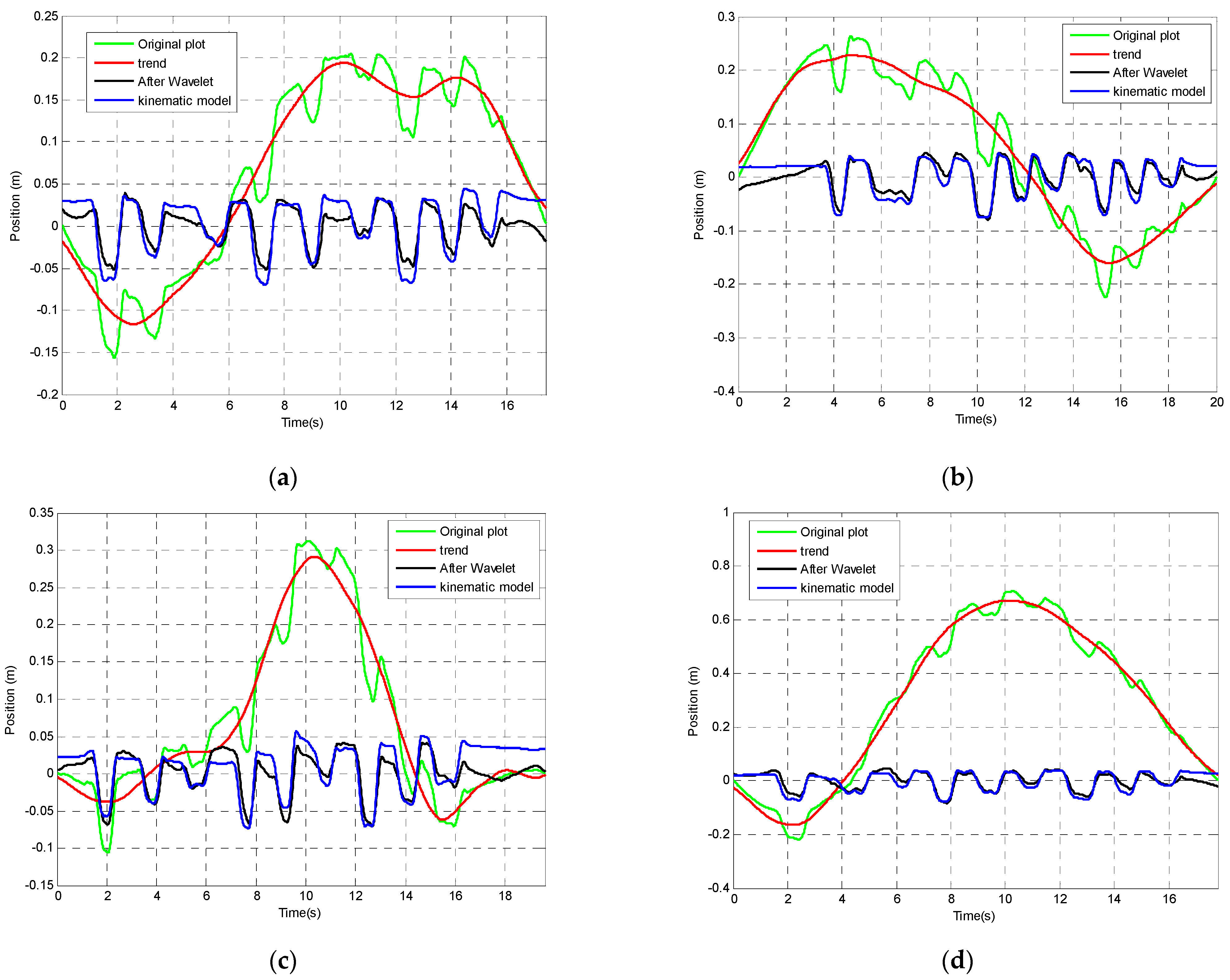
4.2. Results Using Wavelet Analysis
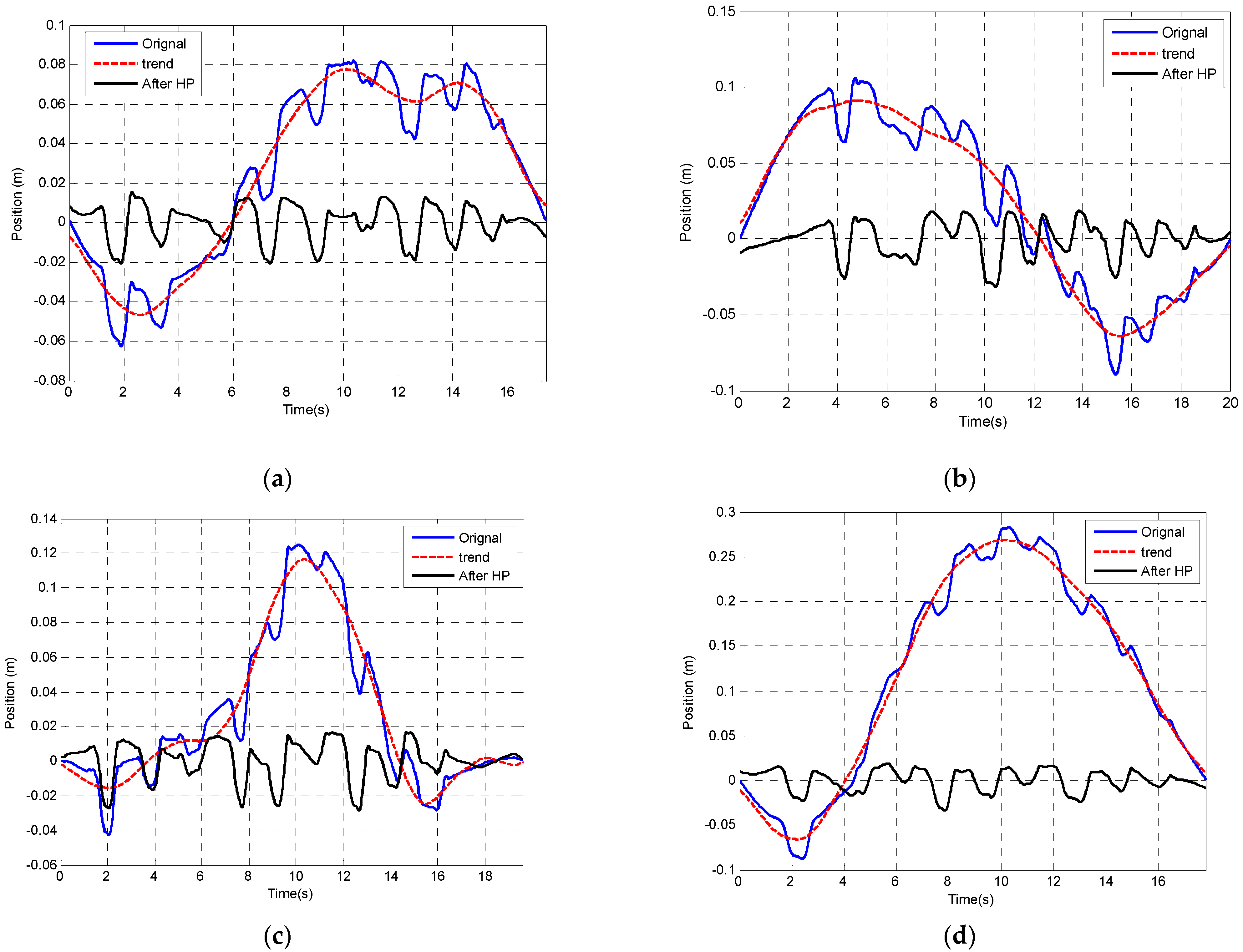
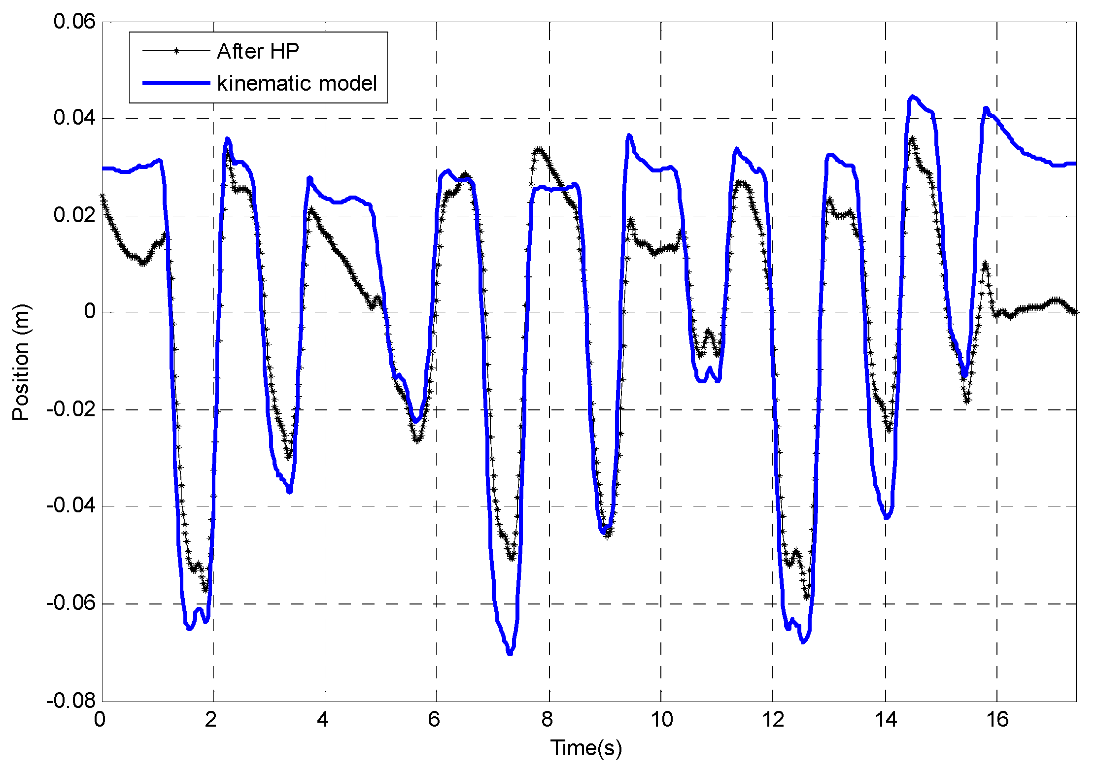
4.3. Results Using HP Filter
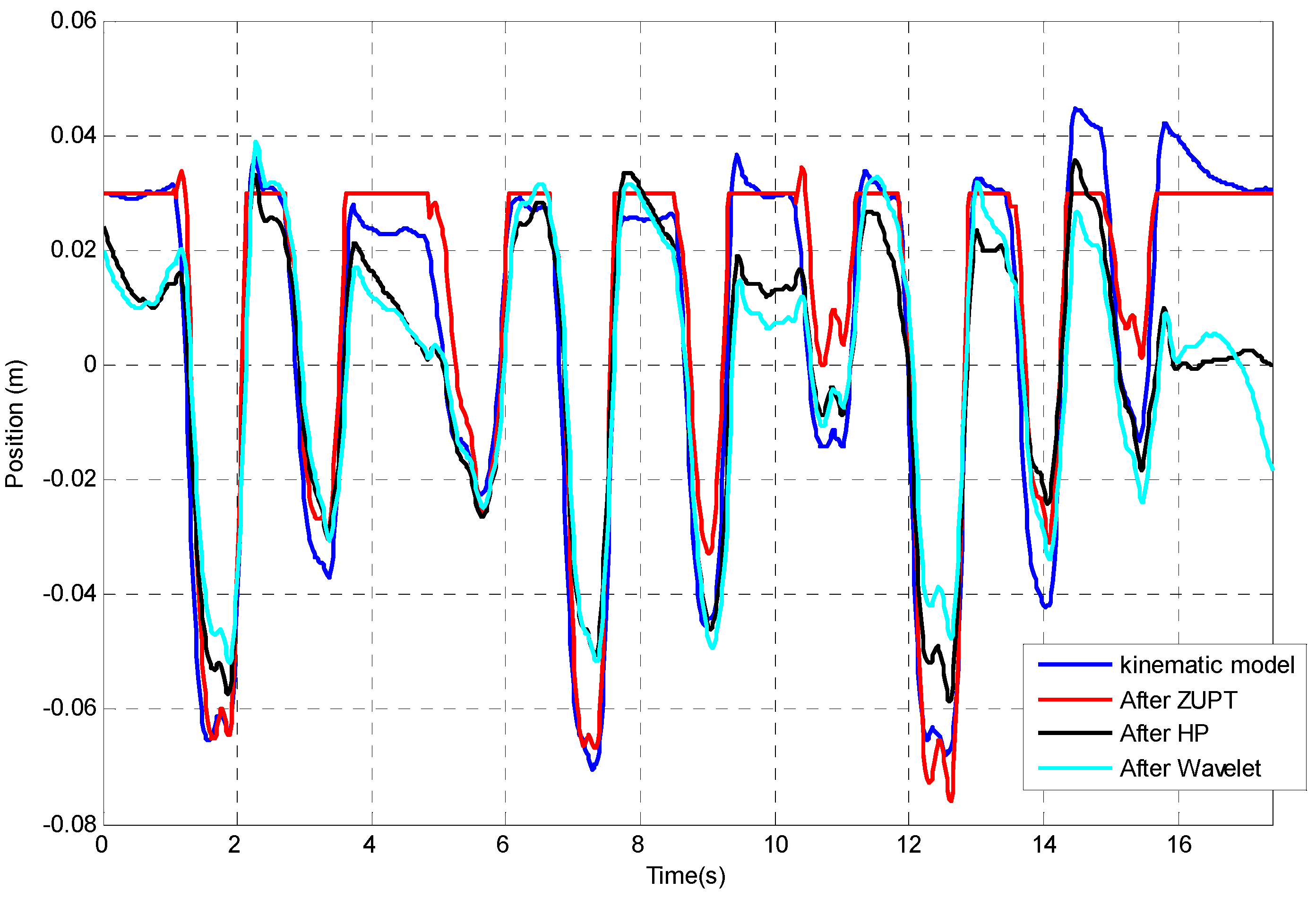
4.4. Comparisons between Different Drifts Correction Methods
5. Conclusions
Author Contributions
Funding
Institutional Review Board Statement
Informed Consent Statement
Data Availability Statement
Conflicts of Interest
References
- Feigin, V.L.; Nichols, E.; Alam, T.; Bannick, M.S.; Beghi, E.; Blake, N.; Culpepper, W.J.; Dorsey, E.R.; Elbaz, A.; Ellenbogen, R.G. Global, regional, and national burden of neurological disorders, 1990–2016: A systematic analysis for the Global Burden of Disease Study 2016. Lancet Neurol. 2019, 18, 459–480. [Google Scholar] [CrossRef] [PubMed] [Green Version]
- NEURO NUMBERS. 2019. Available online: https://www.neural.org.uk/assets/pdfs/neuro-numbers-2019.pdf (accessed on 1 November 2022).
- Tefertiller, C.; Pharo, B.; Evans, N.; Winchester, P. Efficacy of rehabilitation robotics for walking training in neurological disorders:A review. J. Rehabil. Res. Dev. 2011, 48, 387–416. [Google Scholar] [CrossRef] [PubMed]
- Winstein, C.J.; Rose, D.K.; Tan, S.M.; Lewthwaite, R.; Chui, H.C.; Azen, S.P. A randomized controlled comparison of upper-extremity rehabilitation strategies in acute stroke: A pilot study of immediate and long-term outcomes. Arch. Phys. Med. Rehabil. 2004, 85, 620–628. [Google Scholar] [CrossRef] [PubMed]
- Allison, R.; Shenton, L.; Bamforth, K.; Kilbride, C.; Richards, D. Incidence, time course and predictors of impairments relating to caring for the profoundly affected arm after stroke: A systematic review. Physiother. Res. Int. 2016, 21, 210–227. [Google Scholar] [CrossRef] [PubMed] [Green Version]
- Olsen, T.S. Arm and leg paresis as outcome predictors in stroke rehabilitation. Stroke 1990, 21, 247–251. [Google Scholar] [CrossRef] [PubMed] [Green Version]
- Bai, L.; Pepper, M.G.; Yan, Y.; Phillips, M.; Sakel, M. Quantitative measurement of upper limb motion pre- and post-treatment with Botulinum Toxin. Meas. J. Int. Meas. Confed. 2021, 168, 108304. [Google Scholar] [CrossRef]
- Schez-Sobrino, S.; Monekosso, D.N.; Remagnino, P.; Vallejo, D.; Glez-Morcillo, C. Automatic recognition of physical exercises performed by stroke survivors to improve remote rehabilitation. In Proceedings of the 2019 International Conference on Multimedia Analysis and Pattern Recognition (MAPR), Ho Chi Minh City, Vietnam, 9–10 May 2019; pp. 1–6. [Google Scholar]
- Bijalwan, V.; Semwal, V.B.; Singh, G.; Crespo, R.G. Heterogeneous computing model for post-injury walking pattern restoration and postural stability rehabilitation exercise recognition. Expert. Syst. 2022, 39, e12706. [Google Scholar] [CrossRef]
- Kwakkel, G.; Kollen, B.J.; Van der Grond, J.V.; Prevo, A.J.H. Probability of regaining dexterity in the flaccid upper limb: Impact of severity of paresis and time since onset in acute stroke. Stroke 2003, 34, 2181–2186. [Google Scholar] [CrossRef] [Green Version]
- Luke, C.; Dodd, K.J.; Brock, K. Outcomes of the Bobath concept on upper limb recovery following stroke. Clin. Rehabil. 2004, 18, 888–898. [Google Scholar] [CrossRef]
- Barreca, S.; Wolf, S.L.; Fasoli, S.; Bohannon, R. Treatment Interventions for the Paretic Upper Limb of Stroke Survivors: A Critical Review. Neurorehabil. Neural. Repair 2003, 17, 220–226. [Google Scholar] [CrossRef]
- Wu, J.; Cheng, H.; Zhang, J.; Yang, S.; Cai, S. Robot-assisted therapy for upper extremity motor impairment after stroke: A systematic review and meta-analysis. Phys. Ther. 2021, 101, pzab010. [Google Scholar] [CrossRef] [PubMed]
- Ward, N.S.; Brander, F.; Kelly, K. Intensive upper limb neurorehabilitation in chronic stroke: Outcomes from the Queen Square programme. J. Neurol. Neurosurg. Psychiatry 2019, 90, 498–506. [Google Scholar] [CrossRef] [PubMed] [Green Version]
- Maceira-Elvira, P.; Popa, T.; Schmid, A.-C.; Hummel, F.C. Wearable technology in stroke rehabilitation: Towards improved diagnosis and treatment of upper-limb motor impairment. J. Neuroeng. Rehabil. 2019, 16, 142. [Google Scholar] [CrossRef] [PubMed]
- Bai, L.; Pepper, M.G.; Yan, Y.; Phillips, M.; Sakel, M. Low Cost Inertial Sensors for the Motion Tracking and Orientation Estimation of Human Upper Limbs in Neurological Rehabilitation. IEEE Access 2020, 8, 54254–54268. [Google Scholar] [CrossRef]
- Schepers, M. Ambulatory Assessment of Human Body Kinematics and Kinetics; University of Twente: Enschede, The Netherlands, 2015; ISBN 9788578110796. [Google Scholar]
- Bai, L.; Pepper, M.G.; Yan, Y.; Spurgeon, S.K.; Sakel, M.; Phillips, M. Quantitative Assessment of Upper Limb Motion in Neurorehabilitation Utilizing Inertial Sensors. IEEE Trans. Neural. Syst. Rehabil. Eng. 2015, 23, 232–243. [Google Scholar] [CrossRef]
- Filippeschi, A.; Schmitz, N.; Miezal, M.; Bleser, G.; Ruffaldi, E.; Stricker, D. Survey of motion tracking methods based on inertial sensors: A focus on upper limb human motion. Sensors 2017, 17, 1257. [Google Scholar] [CrossRef] [Green Version]
- Schepers, M.; Giuberti, M.; Bellusci, G. Xsens MVN: Consistent tracking of human motion using inertial sensing. Xsens Technol. 2018, 1, 1–8. [Google Scholar]
- Foxlin, E. Inertial head-tracker sensor fusion by a complementary separate-bias Kalman filter. In Proceedings of the Proceedings—Virtual Reality Annual International Symposium, Santa Clara, CA, USA, 30 March–3 April 1996. [Google Scholar]
- Luinge, H.J.; Veltink, P.H. Measuring orientation of human body segments using miniature gyroscopes and accelerometers. Med. Biol. Eng. Comput. 2005, 43, 273–282. [Google Scholar] [CrossRef]
- Roetenberg, D.; Slycke, P.J.; Veltink, P.H. Ambulatory position and orientation tracking fusing magnetic and inertial sensing. IEEE Trans. Biomed. Eng. 2007, 54, 883–890. [Google Scholar] [CrossRef] [Green Version]
- Zhou, H.; Hu, H. Reducing drifts in the inertial measurements of wrist and elbow positions. IEEE Trans. Instrum. Meas. 2010, 59, 575–585. [Google Scholar] [CrossRef]
- Picerno, P.; Caliandro, P.; Iacovelli, C.; Simbolotti, C.; Crabolu, M.; Pani, D.; Vannozzi, G.; Reale, G.; Rossini, P.M.; Padua, L. Upper limb joint kinematics using wearable magnetic and inertial measurement units: An anatomical calibration procedure based on bony landmark identification. Sci. Rep. 2019, 9, 14449. [Google Scholar] [CrossRef] [PubMed]
- Doğan, M.; Koçak, M.; Kılınç, Ö.O.; Ayvat, F.; Sütçü, G.; Ayvat, E.; Kılınç, M.; Ünver, Ö.; Yıldırım, S.A. Functional range of motion in the upper extremity and trunk joints: Nine functional everyday tasks with inertial sensors. Gait Posture 2019, 70, 141–147. [Google Scholar] [CrossRef] [PubMed]
- Chen, H.; Schall, M.C.; Fethke, N.B. Measuring upper arm elevation using an inertial measurement unit: An exploration of sensor fusion algorithms and gyroscope models. Appl. Ergon. 2020, 89, 103187. [Google Scholar] [CrossRef] [PubMed]
- Leuenberger, K.; Gonzenbach, R.; Wachter, S.; Luft, A.; Gassert, R. A method to qualitatively assess arm use in stroke survivors in the home environment. Med. Biol. Eng. Comput. 2017, 55, 141–150. [Google Scholar] [CrossRef] [Green Version]
- Lawrence, A. Modern Inertial Technology: Navigation, Guidance, and Control, 2nd ed.; Springer: New York, NY, USA, 1998. [Google Scholar]
- Tjhai, C.; O’Keefe, K. Comparing heading estimates from multiple wearable inertial and magnetic sensors mounted on lower limbs. In Proceedings of the 2018 International Conference on Indoor Positioning and Indoor Navigation (IPIN), Nantes, France, 24–27 September 2018; pp. 206–212. [Google Scholar]
- Tjhai, C.; O’Keefe, K. Using step size and lower limb segment orientation from multiple low-cost wearable inertial/magnetic sensors for pedestrian navigation. Sensors 2019, 19, 3140. [Google Scholar] [CrossRef] [Green Version]
- Labinghisa, B.; Lee, D.M. Drift-free indoor pedestrian dead reckoning using empirical mode decomposition. In Proceedings of the 2019 25th Asia-Pacific Conference on Communications (APCC), Ho Chi Minh City, Vietnam, 6–8 November 2019; pp. 262–266. [Google Scholar]
- Elbes, M.; Al-Fuqaha, A.; Rayes, A. Gyroscope drift correction based on TDoA technology in support of pedestrian dead reckoning. In Proceedings of the 2012 IEEE Globecom Workshops, Anaheim, CA, USA, 3–7 December 2012; pp. 314–319. [Google Scholar]
- Welte, A.; Xu, P.; Bonnifait, P. Four-Wheeled Dead-Reckoning Model Calibration using RTS Smoothing. In Proceedings of the 2019 International Conference on Robotics and Automation (ICRA), Montreal, QC, Canada, 20–24 May 2019; pp. 312–318. [Google Scholar]
- Tong, X.; Su, Y.; Li, Z.; Si, C.; Han, G.; Ning, J.; Yang, F. A double-step unscented Kalman filter and HMM-based zero-velocity update for pedestrian dead reckoning using MEMS sensors. IEEE Trans. Ind. Electron. 2019, 67, 581–591. [Google Scholar] [CrossRef]
- Lee, J.H.; Cho, S.Y.; Park, C.G. Symmetric position drift of integration approach in pedestrian dead reckoning with dual foot-mounted IMU. J. Position. Navig. Timing. 2020, 9, 117–124. [Google Scholar]
- Pearson, K. The problem of the random walk. Nature 1905, 72, 294. [Google Scholar] [CrossRef]
- Yu, X.; Liu, B.; Lan, X.; Xiao, Z.; Lin, S.; Yan, B.; Zhou, L. AZUPT: Adaptive zero velocity update based on neural networks for pedestrian tracking. In Proceedings of the 2019 IEEE Global Communications Conference (GLOBECOM), Waikoloa, HI, USA, 9–13 December 2019; pp. 1–6. [Google Scholar]
- Skog, I.; Nilsson, J.-O.; Händel, P. Evaluation of zero-velocity detectors for foot-mounted inertial navigation systems. In Proceedings of the 2010 International Conference on indoor positioning and indoor navigation, Zurich, Switzerland, 15–17 September 2010; pp. 1–6. [Google Scholar]
- Vartiainen, J.; Lehtomäki, J.J.; Saarnisaari, H. Double-threshold based narrowband signal extraction. In Proceedings of the IEEE Vehicular Technology Conference, Stockholm, Sweden, 30 May–1 June 2005. [Google Scholar]
- Akansu, A.N.; Serdijn, W.A.; Selesnick, I.W. Emerging applications of wavelets: A review. Phys. Commun. 2010, 3, 1–18. [Google Scholar] [CrossRef]
- Rafiee, J.; Rafiee, M.A.; Prause, N.; Schoen, M.P. Wavelet basis functions in biomedical signal processing. Expert. Syst. Appl. 2011, 38, 6190–6201. [Google Scholar] [CrossRef]
- Christiano, L.J.; Fitzgerald, T.J. The band pass filter. Int. Econ. Rev. 2003, 44, 435–465. [Google Scholar] [CrossRef]
- Mathiowetz, V.; Weber, K.; Kashman, N.; Volland, G. Adult norms for the nine hole peg test of finger dexterity. Occup. Ther. J. Res. 1985, 5, 24–38. [Google Scholar] [CrossRef]
- Woodman, O.J. An introduction to inertial navigation. Univ. Camb. Comput. Lab. 2007, 77, 844–847. [Google Scholar]
- Bai, L.; Pepper, M.G.; Yan, Y.; Spurgeon, S.K.; Sakel, M.; Phillips, M. A multi-parameter assessment tool for upper limb motion in neurorehabilitation. In Proceedings of the Conference Record—IEEE Instrumentation and Measurement Technology Conference, Hangzhou, China, 10–12 May 2011. [Google Scholar]
- Titterton, D.; Weston, J. Strapdown Inertial Navigation Technology; AIAA: Reston, VA, USA, 2004. [Google Scholar]
- Ojeda, L.; Borenstein, J. Personal dead-reckoning system for GPS-denied environments. In Proceedings of the SSRR2007—IEEE International Workshop on Safety, Security and Rescue Robotics Proceedings, Rome, Italy, 27–29 September 2007. [Google Scholar]
- Lu, X.; Liu, R.; Liu, J.; Liang, S. Removal of noise by wavelet method to generate high quality temporal data of terrestrial MODIS products. Photogramm. Eng. Remote Sens. 2007, 73, 1129–1139. [Google Scholar] [CrossRef] [Green Version]
- Xiaofang, L.; Yuliang, M.; Ling, X.; Jiabin, C.; Chunlei, S. Applications of zero-velocity detector and Kalman filter in zero velocity update for inertial navigation system. In Proceedings of the 2014 IEEE Chinese Guidance, Navigation and Control Conference, Yantai, China, 8–10 August 2014; pp. 1760–1763. [Google Scholar]
- Zhao, T.; Ahamed, M.J. Pseudo-Zero Velocity Re-Detection Double Threshold Zero-Velocity Update (ZUPT) for Inertial Sensor-Based Pedestrian Navigation. IEEE Sens. J. 2021, 21, 13772–13785. [Google Scholar] [CrossRef]


| Correlation Coefficient | ZUPT | HP | Wavelet |
|---|---|---|---|
| Kinematic model | 0.97 | 0.92 | 0.88 |
| (cm) | ZUPT | HP | Wavelet |
|---|---|---|---|
| Mean | 0.48 | 0.49 | 0.50 |
| STD | 0.86 | 1.43 | 1.65 |
Disclaimer/Publisher’s Note: The statements, opinions and data contained in all publications are solely those of the individual author(s) and contributor(s) and not of MDPI and/or the editor(s). MDPI and/or the editor(s) disclaim responsibility for any injury to people or property resulting from any ideas, methods, instructions or products referred to in the content. |
© 2022 by the authors. Licensee MDPI, Basel, Switzerland. This article is an open access article distributed under the terms and conditions of the Creative Commons Attribution (CC BY) license (https://creativecommons.org/licenses/by/4.0/).
Share and Cite
Bai, L.; Pepper, M.G.; Wang, Z.; Mulvenna, M.D.; Bond, R.R.; Finlay, D.; Zheng, H. Upper Limb Position Tracking with a Single Inertial Sensor Using Dead Reckoning Method with Drift Correction Techniques. Sensors 2023, 23, 360. https://doi.org/10.3390/s23010360
Bai L, Pepper MG, Wang Z, Mulvenna MD, Bond RR, Finlay D, Zheng H. Upper Limb Position Tracking with a Single Inertial Sensor Using Dead Reckoning Method with Drift Correction Techniques. Sensors. 2023; 23(1):360. https://doi.org/10.3390/s23010360
Chicago/Turabian StyleBai, Lu, Matthew G. Pepper, Zhibao Wang, Maurice D. Mulvenna, Raymond R. Bond, Dewar Finlay, and Huiru Zheng. 2023. "Upper Limb Position Tracking with a Single Inertial Sensor Using Dead Reckoning Method with Drift Correction Techniques" Sensors 23, no. 1: 360. https://doi.org/10.3390/s23010360