
Non-Destructive Testing for Cavity Damages in Automated Machines Based on Acoustic Emission Tomography


Abstract
:1. Introduction
2. Methods
2.1. Forward Modeling
- Initialization: initializing the model with , and assigning large positive values at all other grid points;
- Gauss-Seidel iteration: sweeping the domain by Gauss-Seidel iterations, and selecting the smaller value between the new solution and the original solution;
- Convergence: repeating step (2) until .
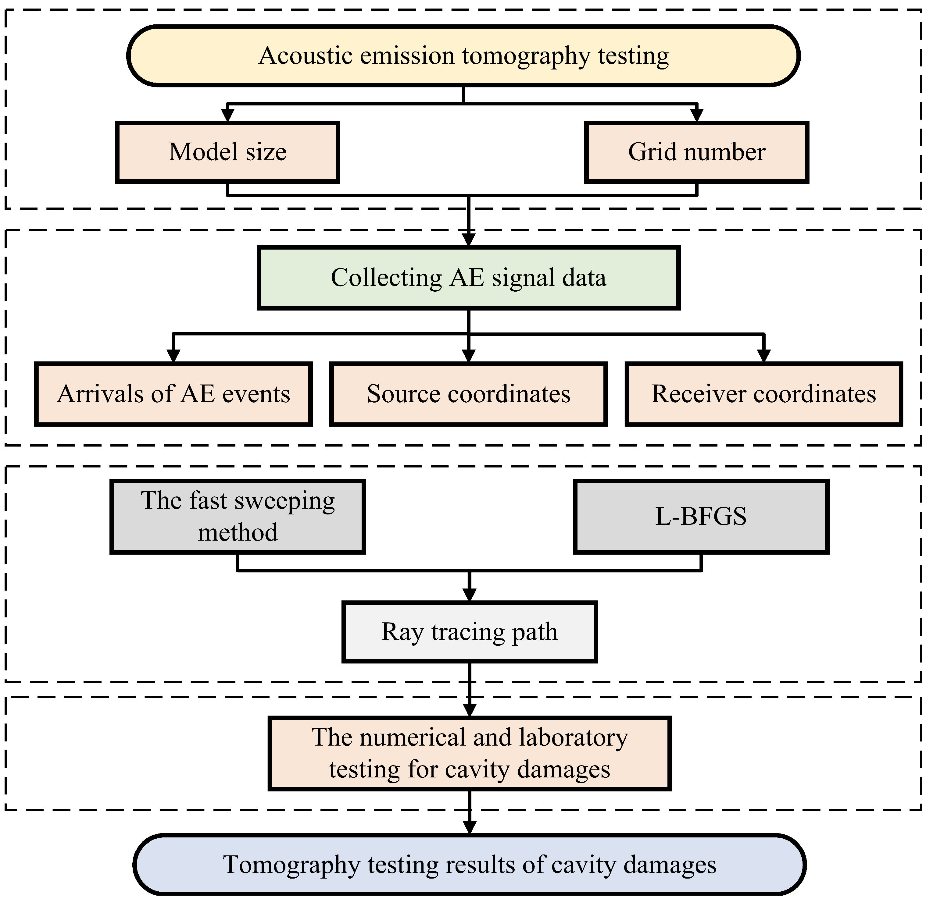
2.2. Inversion
- Establishing the initial model and its grid size according the region of interest;
- Collecting AE signal data, such as arrivals of AE events, source and receiver coordinates;
- Calculating the inversion result from the initial model, based on FSM and L-BFGS, until it satisfies the convergence requirement. The convergence requirement is set so that when the difference of the updated value of the model is smaller than a certain value, or the iteration reaches a certain value, the inversion process is regarded as satisfying the convergence.
3. Experiments
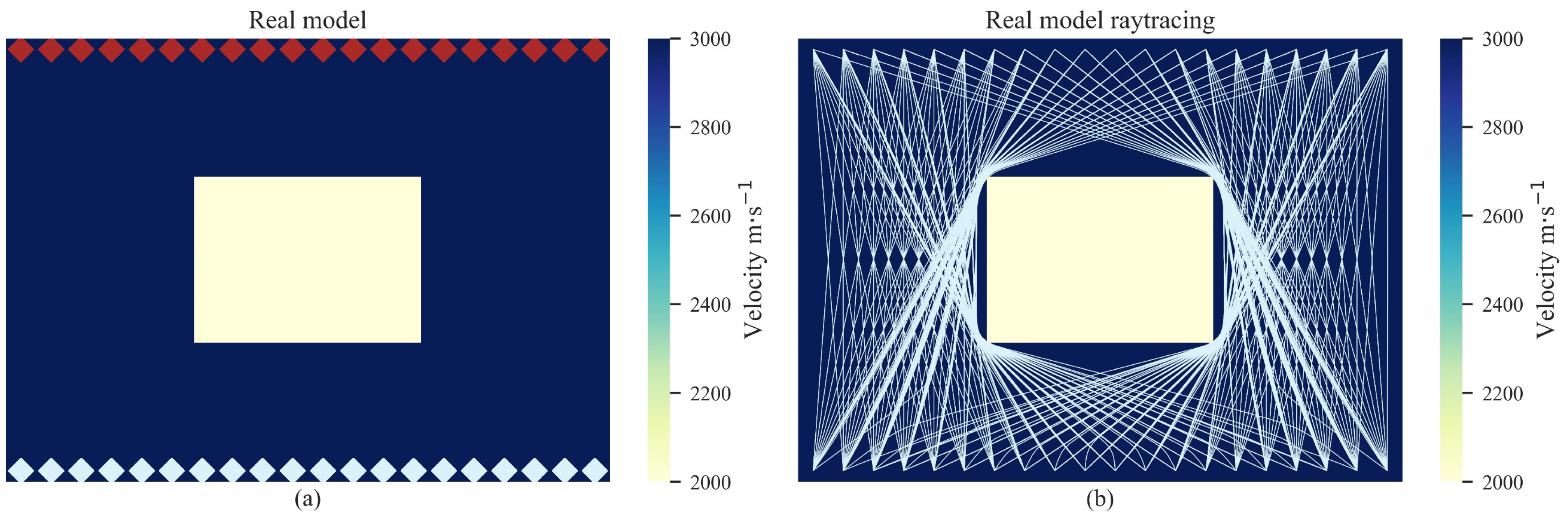
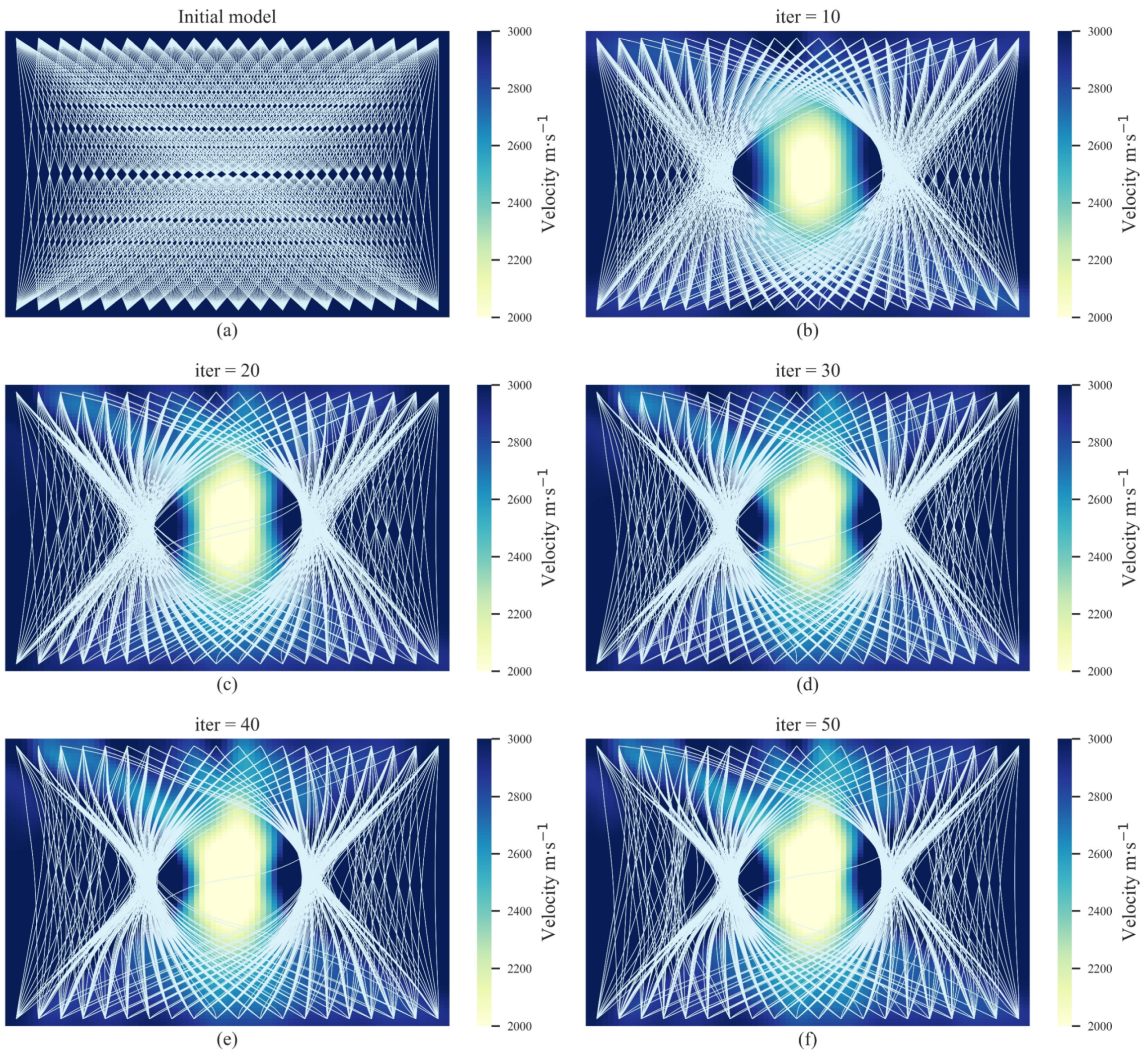
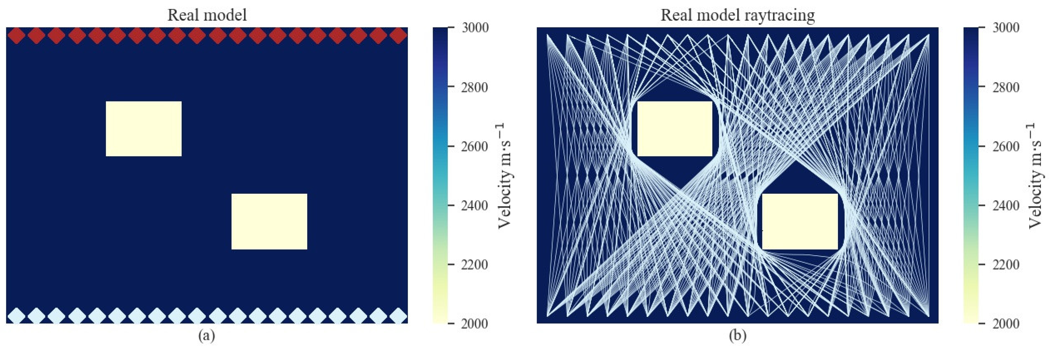
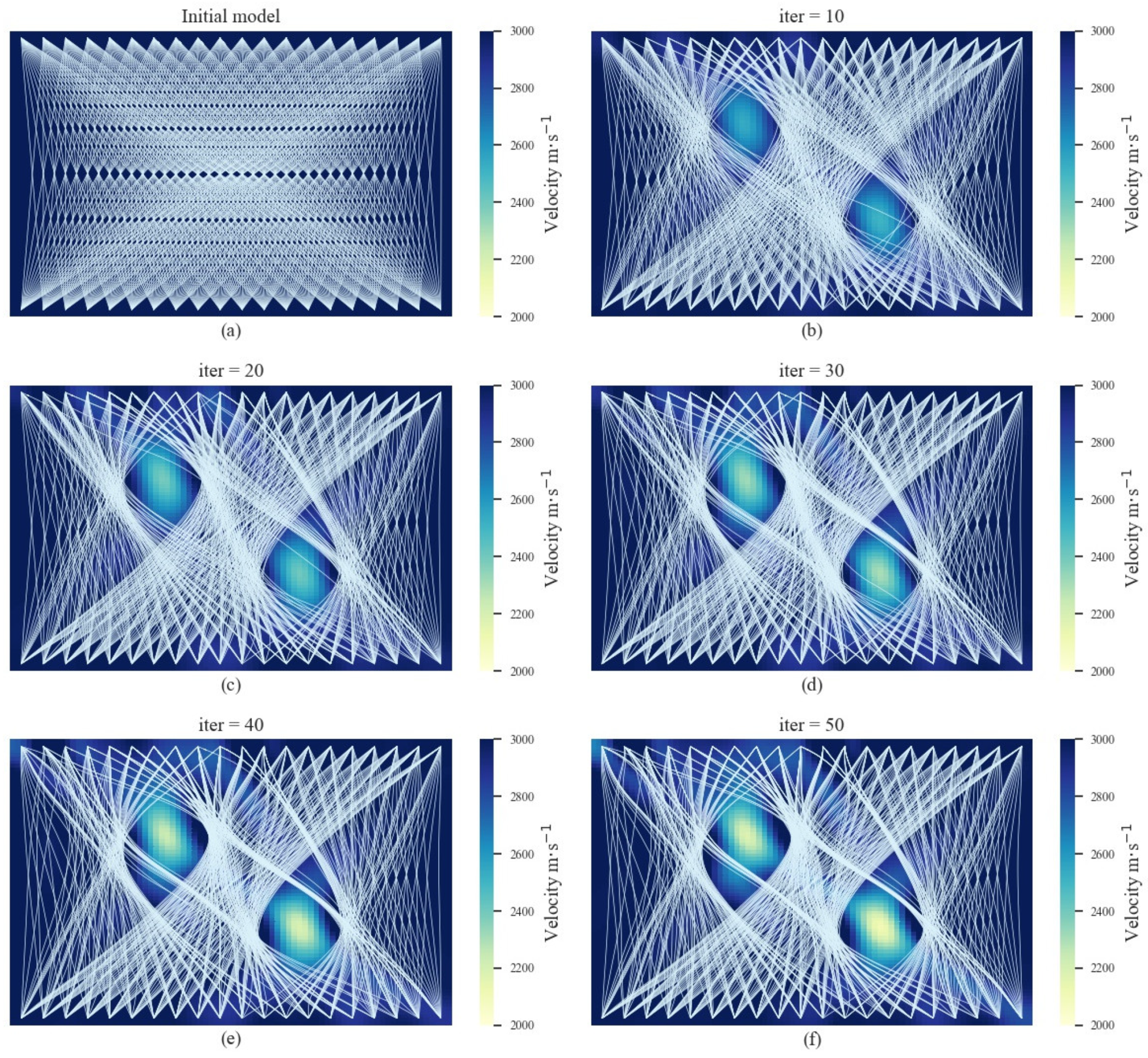
3.1. Numerical Experiments
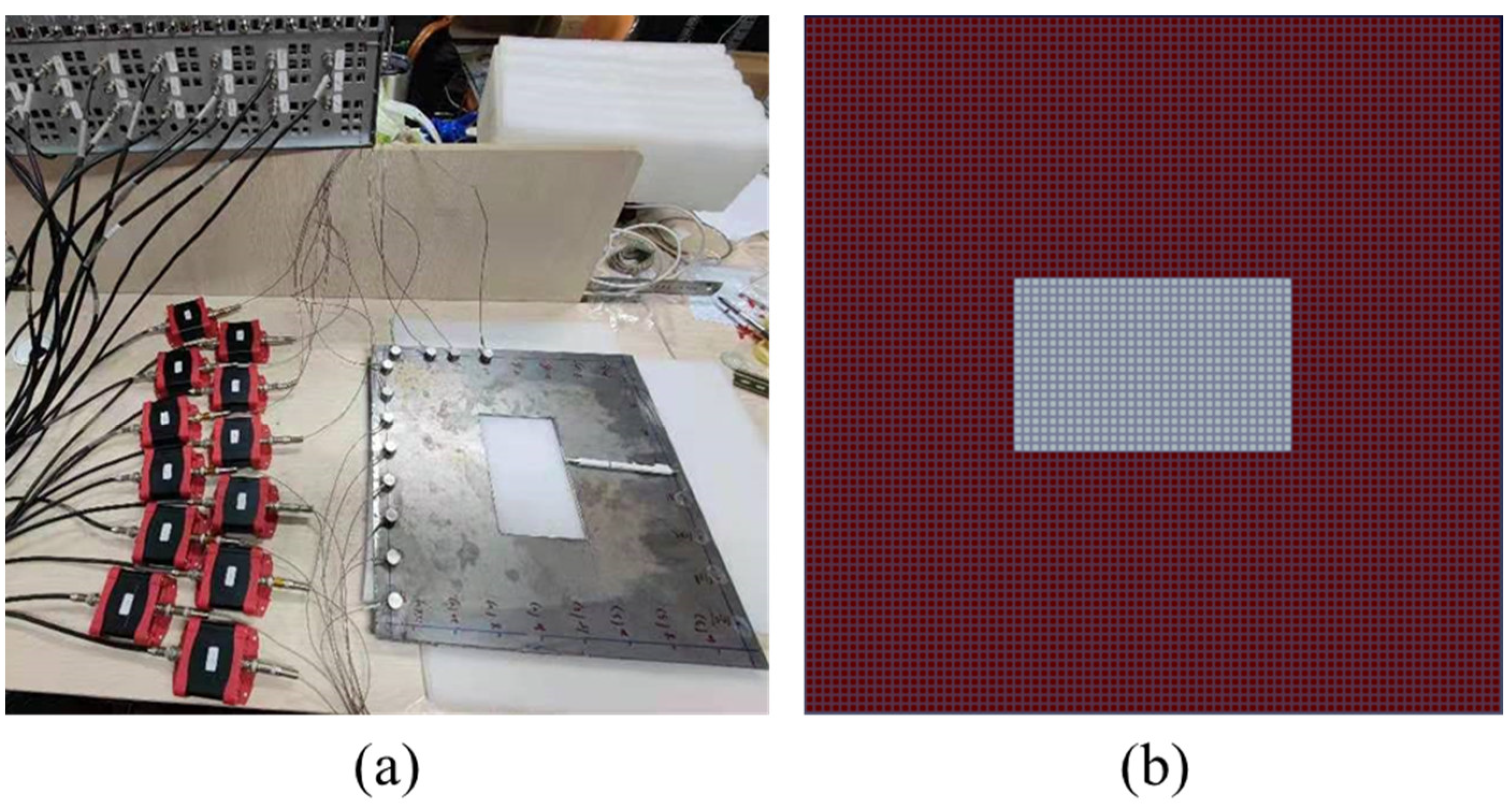
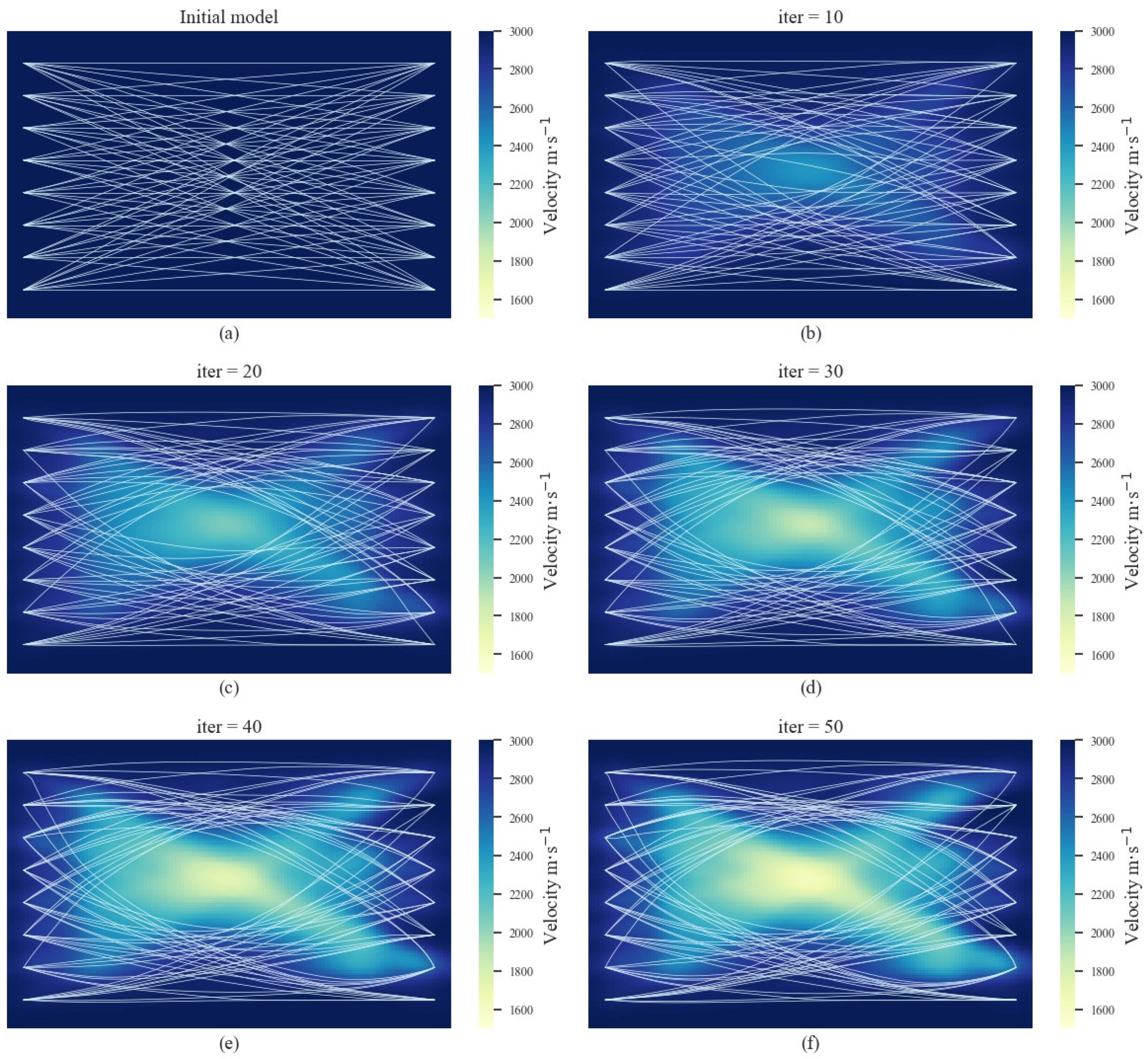
3.2. Laboratory Experiments
4. Conclusions
Author Contributions
Funding
Institutional Review Board Statement
Informed Consent Statement
Data Availability Statement
Conflicts of Interest
References
- Cerrada, M.; Sánchez, R.-V.; Li, C.; Pacheco, F.; Cabrera, D.; Valente de Oliveira, J.; Vásquez, R.E. A review on data-driven fault severity assessment in rolling bearings. Mech. Syst. Signal Process. 2018, 99, 169–196. [Google Scholar] [CrossRef]
- Goyal, D.; Choudhary, A.; Pabla, B.S.; Dhami, S.S. Support vector machines based non-contact fault diagnosis system for bearings. J. Intell. Manuf. 2020, 31, 1275–1289. [Google Scholar] [CrossRef]
- Lei, Y.; Lin, J.; He, Z.; Zuo, M.J. A review on empirical mode decomposition in fault diagnosis of rotating machinery. Mech. Syst. Signal Process. 2013, 35, 108–126. [Google Scholar] [CrossRef]
- Hamzeloo, S.R.; Shamshirsaz, M.; Rezaei, S.M. Damage detection on hollow cylinders by Electro-Mechanical Impedance method: Experiments and Finite Element Modeling. Comptes Rendus Mécanique 2012, 340, 668–677. [Google Scholar] [CrossRef]
- Zolfaghari, A.; Zolfaghari, A.; Kolahan, F. Reliability and sensitivity of magnetic particle nondestructive testing in detecting the surface cracks of welded components. Nondestruct. Test. Eval. 2018, 33, 290–300. [Google Scholar] [CrossRef]
- Tout, K.; Meguenani, A.; Urban, J.-P.; Cudel, C. Automated vision system for magnetic particle inspection of crankshafts using convolutional neural networks. Int. J. Adv. Manuf. Technol. 2021, 112, 3307–3326. [Google Scholar] [CrossRef]
- Zhang, M.; Zhang, X.; Li, M.; Cao, J.; Huang, Z. Optimization Design and Flexible Detection Method of a Surface Adaptation Wall-Climbing Robot with Multisensor Integration for Petrochemical Tanks. Sensors 2020, 20, 6651. [Google Scholar] [CrossRef] [PubMed]
- Wang, X.; Wong, B.S.; Tan, C.; Tui, C.G. Automated Crack Detection for Digital Radiography Aircraft Wing Inspection. Res. Nondestruct. Eval. 2011, 22, 105–127. [Google Scholar] [CrossRef]
- Rifai, D.; Abdalla, A.; Ali, K.; Razali, R. Giant Magnetoresistance Sensors: A Review on Structures and Non-Destructive Eddy Current Testing Applications. Sensors 2016, 16, 298. [Google Scholar] [CrossRef] [Green Version]
- Dong, L.; Zou, W.; Li, X.; Shu, W.; Wang, Z. Collaborative localization method using analytical and iterative solutions for microseismic/acoustic emission sources in the rockmass structure for underground mining. Eng. Fract. Mech. 2019, 210, 95–112. [Google Scholar] [CrossRef]
- Dong, L.; Zhang, Y.; Ma, J. Micro-Crack Mechanism in the Fracture Evolution of Saturated Granite and Enlightenment to the Precursors of Instability. Sensors 2020, 20, 4595. [Google Scholar] [CrossRef] [PubMed]
- Ma, J.; Dong, L.; Zhao, G.; Li, X. Focal Mechanism of Mining-Induced Seismicity in Fault Zones: A Case Study of Yongshaba Mine in China. Rock Mech. Rock Eng. 2019, 52, 3341–3352. [Google Scholar] [CrossRef]
- Krause, T.; Ostermann, J. Damage detection for wind turbine rotor blades using airborne sound. Struct. Control Health Monit. 2020, 27, e2520. [Google Scholar] [CrossRef]
- Dong, L.; Chen, Y.; Sun, D.; Zhang, Y. Implications for rock instability precursors and principal stress direction from rock acoustic experiments. Int. J. Min. Sci. Technol. 2021, 31, 789–798. [Google Scholar] [CrossRef]
- Zhao, P.; Sun, Y.; Jiao, J.; Fang, G. Correlation between acoustic emission detection and microstructural characterization for damage evolution. Eng. Fract. Mech. 2020, 230, 106967. [Google Scholar] [CrossRef]
- Dong, L.; Hu, Q.; Tong, X.; Liu, Y. Velocity-Free MS/AE Source Location Method for Three-Dimensional Hole-Containing Structures. Engineering 2020, 6, 827–834. [Google Scholar] [CrossRef]
- Wei, X.; Chen, Y.; Lu, C.; Chen, G.; Huang, L.; Li, Q. Acoustic emission source localization method for high-speed train bogie. Multimed. Tools Appl. 2020, 79, 14933–14949. [Google Scholar] [CrossRef]
- Dong, L.; Tao, Q.; Hu, Q. Influence of temperature on acoustic emission source location accuracy in underground structure. Trans. Nonferrous Met. Soc. China 2021, 31, 2468–2478. [Google Scholar] [CrossRef]
- Dong, L.; Tao, Q.; Hu, Q.; Deng, S.; Chen, Y.; Luo, Q.; Zhang, X. Acoustic emission source location method and experimental verification for structures containing unknown empty areas. Int. J. Min. Sci. Technol. 2022. [Google Scholar] [CrossRef]
- Pei, N.; Shang, J.; Bond, L.J. Analysis of Progressive Tensile Damage of Multi-walled Carbon Nanotube Reinforced Carbon Fiber Composites by Using Acoustic Emission and Micro-CT. J. Nondestruct. Eval. 2021, 40, 51. [Google Scholar] [CrossRef]
- Yang, J.; Mu, Z.-L.; Yang, S.-Q. Experimental study of acoustic emission multi-parameter information characterizing rock crack development. Eng. Fract. Mech. 2020, 232, 107045. [Google Scholar] [CrossRef]
- Al-Jumaili, S.K.; Eaton, M.J.; Holford, K.M.; Pearson, M.R.; Crivelli, D.; Pullin, R. Characterisation of fatigue damage in composites using an Acoustic Emission Parameter Correction Technique. Compos. Part B Eng. 2018, 151, 237–244. [Google Scholar] [CrossRef] [Green Version]
- Jiang, Y.; Xu, F.; Xu, B. Acoustic Emission tomography based on simultaneous algebraic reconstruction technique to visualize the damage source location in Q235B steel plate. Mech. Syst. Signal Process. 2015, 64–65, 452–464. [Google Scholar] [CrossRef]
- Dong, L.; Tong, X.; Hu, Q.; Tao, Q. Empty region identification method and experimental verification for the two-dimensional complex structure. Int. J. Rock Mech. Min. Sci. 2021, 147, 104885. [Google Scholar] [CrossRef]
- Brantut, N. Time-resolved tomography using acoustic emissions in the laboratory, and application to sandstone compaction. Geophys. J. Int. 2018, 213, 2177–2192. [Google Scholar] [CrossRef]
- Zhao, H. A fast sweeping method for Eikonal equations. Math. Comput. 2004, 74, 603–627. [Google Scholar] [CrossRef] [Green Version]
- Leung, S.; Qian, J. An adjoint state method for three-dimensional transmission traveltime tomography using first-arrivals. Commun. Math. Sci. 2006, 4, 249–266. [Google Scholar] [CrossRef] [Green Version]


Publisher’s Note: MDPI stays neutral with regard to jurisdictional claims in published maps and institutional affiliations. |
© 2022 by the authors. Licensee MDPI, Basel, Switzerland. This article is an open access article distributed under the terms and conditions of the Creative Commons Attribution (CC BY) license (https://creativecommons.org/licenses/by/4.0/).
Share and Cite
Su, Y.; Dong, L.; Pei, Z. Non-Destructive Testing for Cavity Damages in Automated Machines Based on Acoustic Emission Tomography. Sensors 2022, 22, 2201. https://doi.org/10.3390/s22062201
Su Y, Dong L, Pei Z. Non-Destructive Testing for Cavity Damages in Automated Machines Based on Acoustic Emission Tomography. Sensors. 2022; 22(6):2201. https://doi.org/10.3390/s22062201
Chicago/Turabian StyleSu, Yueyuan, Longjun Dong, and Zhongwei Pei. 2022. "Non-Destructive Testing for Cavity Damages in Automated Machines Based on Acoustic Emission Tomography" Sensors 22, no. 6: 2201. https://doi.org/10.3390/s22062201