
Multi-Filter Clustering Fusion for Feature Selection in Rotating Machinery Fault Classification

 , , ,
, , ,
Abstract
:1. Introduction
2. Related Methods
2.1. Feature Selection Methods
2.2. Classifiers
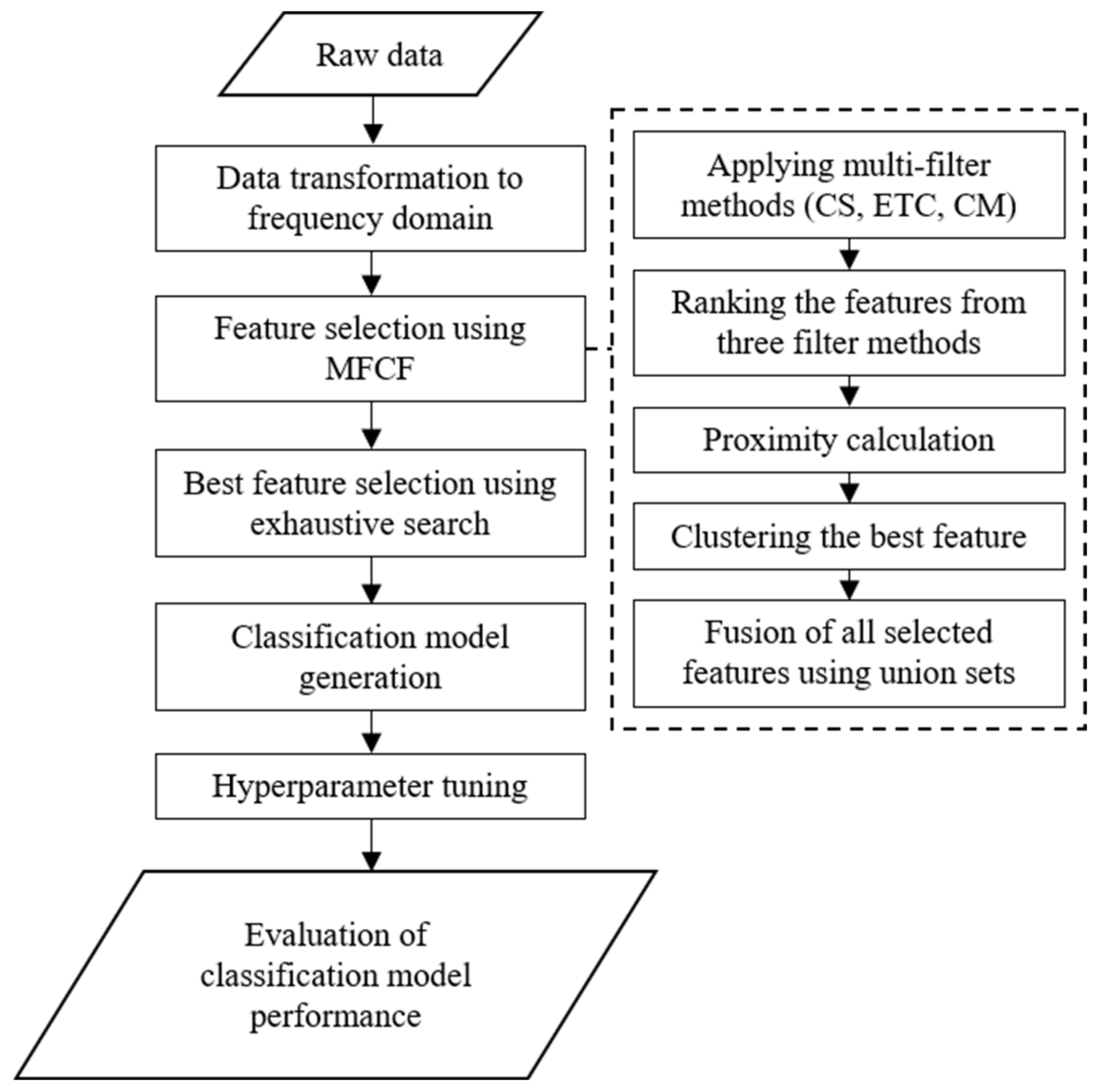
3. Proposed Method
3.1. Fusion Multi-Filter Feature Selection
3.2. Exhaustive Search Application
4. Case Studies
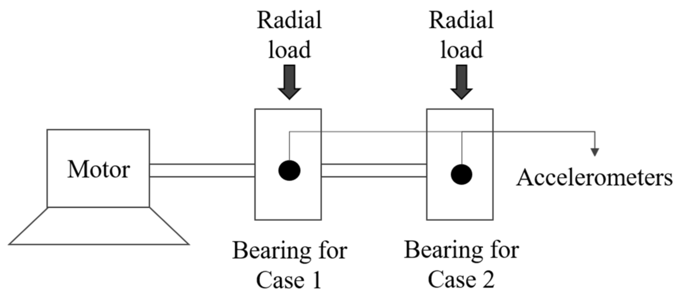
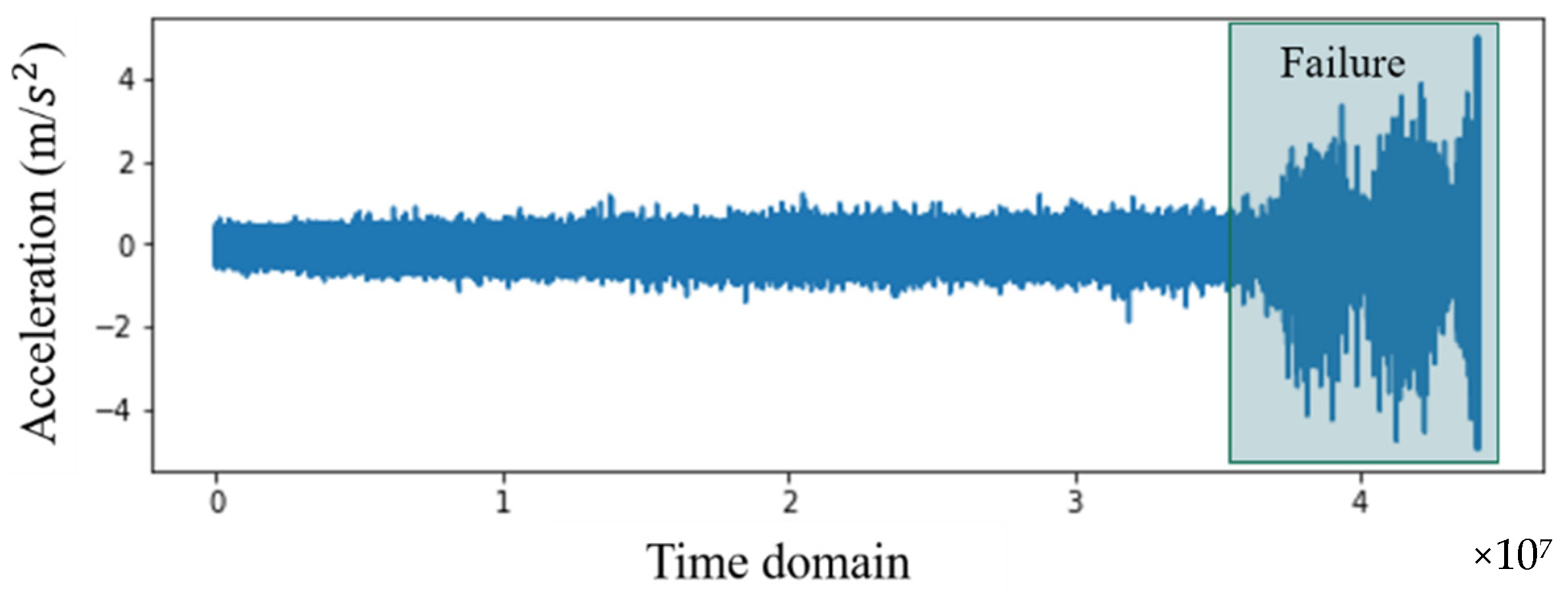
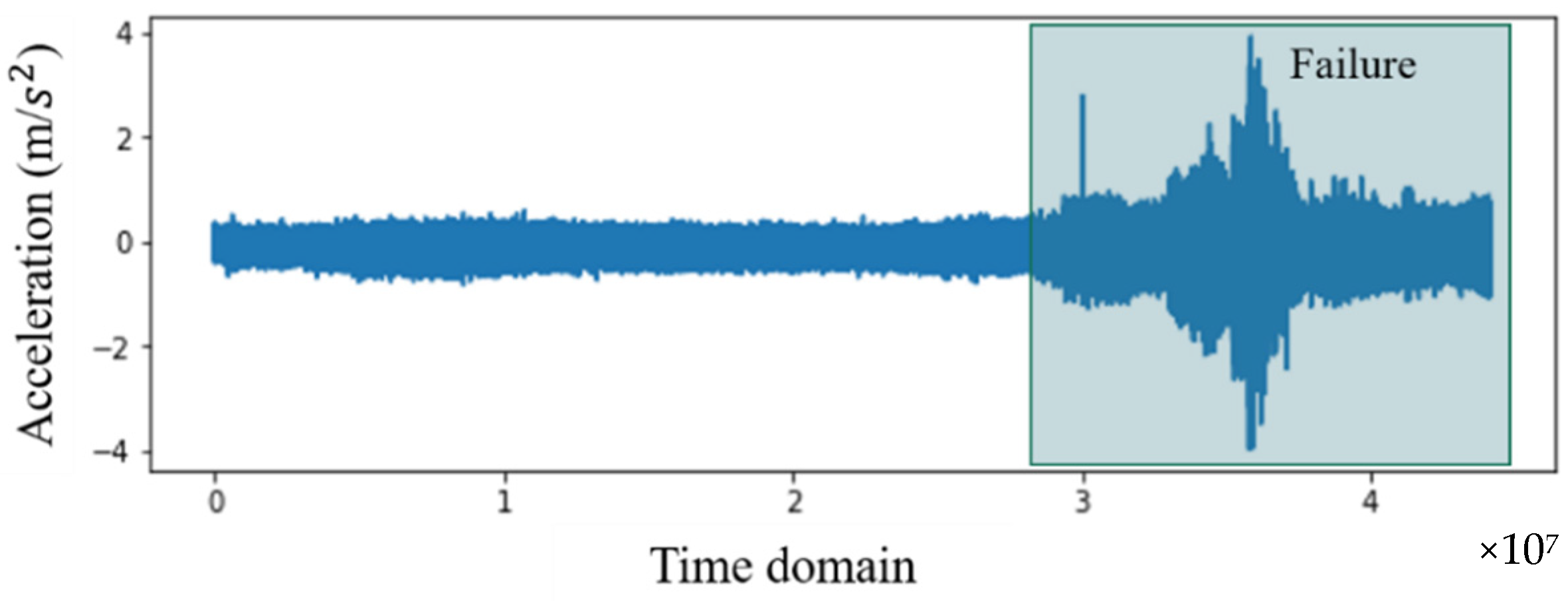
4.1. Data Collection
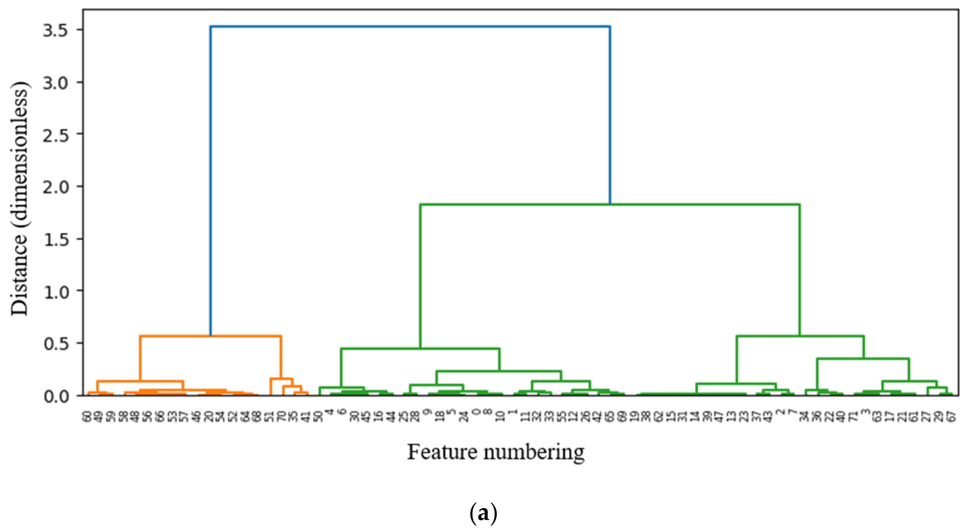
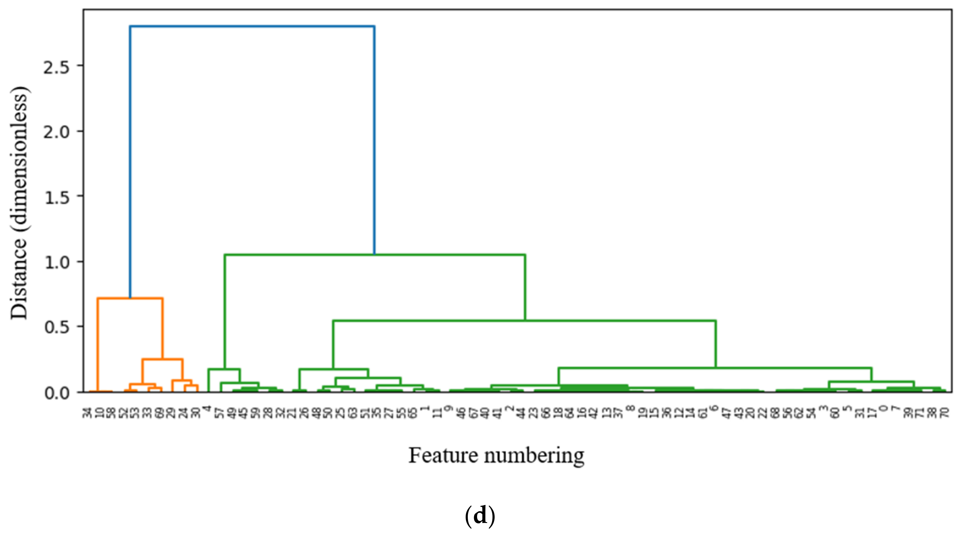
4.2. Feature Extraction and Selection
5. Conclusions
Author Contributions
Funding
Institutional Review Board Statement
Informed Consent Statement
Data Availability Statement
Conflicts of Interest
References
- Cheng, J.; Yang, Y.; Hu, N.; Cheng, Z.; Cheng, J. A noise reduction method based on adaptive weighted symplectic geometry decomposition and its application in early gear fault diagnosis. Mech. Syst. Signal Process. 2021, 149, 107351. [Google Scholar] [CrossRef]
- Li, X.; Yang, Y.; Hu, Z.; Cheng, J.; Cheng, J. Discriminative manifold random vector functional link neural network for rolling bearing fault diagnosis. Knowl.-Based Syst. 2021, 211, 106507. [Google Scholar] [CrossRef]
- Fuli, Y.L.; Jia, W.M.; Qi, Y. Centrifugal compressor fault diagnosis based on qualitative simulation and thermal parameters. Mech. Syst. Signal Process. 2016, 8, 259–273. [Google Scholar] [CrossRef]
- Li, X.; Yang, Y.; Pan, H.; Cheng, J.; Cheng, J. A novel deep stacking least squares support vector machine for rolling bearing fault diagnosis. Comput. Ind. 2019, 110, 36–47. [Google Scholar] [CrossRef]
- Yang, B.; Lei, Y.; Jia, F.; Xing, S. An intelligent fault diagnosis approach based on transfer learning from laboratory bearings to locomotive bearings. Mech. Syst. Signal Process. 2019, 122, 692–706. [Google Scholar] [CrossRef]
- Li, X.; Yang, Y.; Shao, H.; Zhong, X.; Cheng, J.; Cheng, J. Symplectic weighted sparse support matrix machine for gear fault diagnosis. Measurement 2021, 168, 108392. [Google Scholar] [CrossRef]
- Gao, Y.; Yu, D. Total variation on horizontal visibility graph and its application to rolling bearing fault diagnosis. Mech. Mach. Theory 2020, 147, 103768. [Google Scholar] [CrossRef]
- Youwei, W.; Lizhou, F. Hybrid feature selection using component co-occurrence based feature relevance measurement. Expert Syst. Appl. 2018, 102, 83–99. [Google Scholar]
- Uysal, A.K.; Gunal, S. A novel probabilistic feature selection method for text classification. Knowl.-Based Syst. 2021, 36, 226–235. [Google Scholar] [CrossRef]
- Dimitrios, E.; Avi, A. An evaluation of feature selection methods for environmental data. Ecol. Inform. J. 2021, 61, 101224. [Google Scholar]
- Abdelhamid, N.; Thabtah, F.; Abdel-Jaber, H. Phishing detection: A recent intelligent machine learning comparison based on models content and features. In Proceedings of the 2017 IEEE International Conference on Intelligence and Security Informatics: Security and Big Data (ISI), Beijing, China, 22–24 July 2017; pp. 72–77. [Google Scholar]
- Kamalov, F.; Thabtah, F. A feature selection method based on ranked vector scores of features for classification. Ann. Data Sci. 2017, 4, 483–502. [Google Scholar] [CrossRef]
- Sánchez, R.; Lucero, P.; Vasquez, R.; Cerrada, M.; Macancela, J.; Cebrera, D. Feature ranking for multi-fault diagnosis of rotating machinery by using random forest and KNN. J. Intell. Fuzzy Syst. 2018, 34, 3463–3473. [Google Scholar] [CrossRef]
- Ziani, R.; Mahgoun, H.; Fedala, S.; Felkaoui, A. Feature selection scheme based on Pareto method for gearbox fault diagnosis. Signal Process. Appl. Rotating Mach. Diagn. 2017, 12, 1–15. [Google Scholar]
- Zhang, X.; Zhang, Q.; Chen, M.; Sun, Y.; Qin, X.; Li, H. A two-stage feature selection and intelligent fault diagnosis method for rotating machinery using hybrid filter and wrapper method. Neurocomputing 2018, 275, 2426–2439. [Google Scholar] [CrossRef]
- Hui, K.; Ooi, C.; Lim, M.; Leong, M.; Al-Obaidi, S. An improved wrapper-based feature selection method for machinery fault diagnosis. PLoS ONE 2017, 12, e0189143. [Google Scholar] [CrossRef] [Green Version]
- Lu, N.; Zhang, G.; Xiao, Z.; Malik, O.P. Feature extraction based on adaptive multiwavelets and LTSA for rotating machinery fault diagnosis. Shock. Vib. 2019, 2019, 1201084. [Google Scholar] [CrossRef] [Green Version]
- Cerrada, M.; Sánchez, M.R.V.; Cabrera, D.; Zurita, G.; Li, C. Multi-stage feature selection by using genetic algorithms for fault diagnosis in gearboxes based on vibration signal. Sensors 2015, 15, 23903–23926. [Google Scholar] [CrossRef] [Green Version]
- Huang, K.; Wu, S.; Li, F.; Yang, C.; Gui, W. Fault diagnosis of hydraulic systems based on deep learning model with multirate data samples. IEEE Trans. Neural Netw. Learn. Syst. 2021, 1–13. [Google Scholar] [CrossRef]
- Zhang, W.; Li, X.; Ma, H.; Luo, Z.; Li, X. Universal domain adaptation in fault diagnostics with hybrid weighted deep adversarial learning. IEEE Trans. Ind. Inform. 2021, 17, 7957–7967. [Google Scholar] [CrossRef]
- Kang, L.C.; Choon, L.T.; Kok, S.W.; Kelvin, S.C.Y.; Wei, K.T. A new hybrid ensemble feature selection framework for machine learning-based phishing detection system. Inf. Sci. 2019, 484, 153–166. [Google Scholar]
- Amir, E.; Adel, K.; David, Y. Data-driven fault detection and diagnosis for packaged rooftop units using statistical machine learning classification methods. Energy Build. 2020, 225, 110318. [Google Scholar]
- Andrea, B.; Xudong, S.; Bernd, B.; Jörg, R.; Michel, L. Benchmark for filter methods for feature selection in high-dimensional classification data. Comput. Stat. Data Anal. 2020, 143, 106839. [Google Scholar]
- Liu, C.; Jiang, D.; Yang, W. Global geometric similarity scheme for feature selection in fault diagnosis. Expert Syst. Appl. 2014, 41, 3585–3595. [Google Scholar] [CrossRef]
- Cortizo, J.C.; Giraldez, I. Multi criteria wrapper improvements to naive bayes learning. In Proceedings of the International Conference on Intelligent Data Engineering and Automated Learning, Burgos, Spain, 20–23 September 2006; pp. 419–427. [Google Scholar]
- Wang, Y.; Feng, L.; Li, Y. Two-step based feature selection method for filtering redundant information. J. Intell. Fuzzy Syst. 2017, 33, 2059–2073. [Google Scholar] [CrossRef]
- Zorarpacı, E.O.; Selma, A. A hybrid approach of differential evolution and artificial bee colony for feature selection. Expert Syst. Appl. 2016, 62, 91–103. [Google Scholar] [CrossRef]
- Samanta, B. Gear fault detection using artificial neural network and support vector machines with genetic algorithms. Mech. Syst. Signal Process. 2004, 12, 625–644. [Google Scholar] [CrossRef]
- Rafiee, J.; Arvani, F.; Harifi, A.; Sadeghi, M.H. Intelligent condition monitoring of a gearbox using artificial neural network. Mech. Syst. Signal Process. 2007, 21, 1746–1754. [Google Scholar] [CrossRef]
- Wu, J.D.; Hsu, C.C. Fault gear identification using vibration signal with discrete wavelet transform technique and fuzzy-logic inference. Expert Syst. Appl. 2009, 36, 3785–3794. [Google Scholar] [CrossRef]
- Dong, X.; Wang, C.; Si, W. ECG beat classification via deterministic learning. Neurocomputing 2017, 240, 112. [Google Scholar] [CrossRef]
- Jha, C.K.; Kolekar, M.H. Cardiac arrhythmia classification using tunable Q-wavelet transform based features and support vector machine classier. Biomed. Signal Process. Control 2020, 59, 101875. [Google Scholar] [CrossRef]
- Sun, K.; Wu, X.; Xue, J.; Ma, F. Development of a new multi-layer perceptron based soft sensor for SO2 emissions in power plant. J. Process Control 2019, 84, 182191. [Google Scholar] [CrossRef]
- Wang, Z.Y.; Lu, C.; Zhou, B. Fault diagnosis for rotary machinery with selective ensemble neural networks. Mech. Syst. Signal Process. 2018, 113, 112–130. [Google Scholar] [CrossRef]
- IMS Bearings Dataset. 2021. Available online: https://ti.arc.nasa.gov/tech/dash/groups/pcoe/prognostic-data-repository/ (accessed on 1 January 2021).
- Ali, J.B.; Saidi, L.; Mouelihi, A.; Chebel-Morello, B.; Fnaiech, F. Linear feature selection and classification using PNN and SFAM neural networks for a nearly online diagnosis of bearing naturally progressing degradations. Eng. App. Artif. Intell. 2015, 42, 67–81. [Google Scholar]
- Duong, B.P.; Khan, S.A.; Shon, D.; Im, K.; Park, J.; Lim, D.S.; Jang, B.; Kim, J.M. A reliable health indicator for fault prognosis of bearings. Sensors 2018, 18, 3740. [Google Scholar] [CrossRef] [Green Version]
- Mochammad, S.; Kang, Y.-J.; Noh, Y.; Park, S.; Ahn, B. Stable hybrid feature selection method for compressor fault diagnosis. IEEE Access 2021, 9, 97415–97429. [Google Scholar] [CrossRef]
- Kim, S.; Noh, Y.; Kang, Y.-J.; Park, S.; Ahn, B. Fault classification model based on time domain feature extraction of vibration data. J. Comp. Struct. Eng. Inst. Korea 2021, 34, 25–33. [Google Scholar] [CrossRef]


| Frequency Domain Features | Time Domain Features | ||||||
|---|---|---|---|---|---|---|---|
| abs_mean_F | 0 | 24 | 48 | abs_mean_T | 12 | 36 | 60 |
| peak_m_F | 1 | 25 | 49 | peak_m_T | 13 | 37 | 61 |
| kur_F | 2 | 26 | 50 | kur_T | 14 | 38 | 62 |
| skew_F | 3 | 27 | 51 | skew_T | 15 | 39 | 63 |
| rms_F | 4 | 28 | 52 | rms_T | 16 | 40 | 64 |
| mean_F | 5 | 29 | 53 | mean_T | 17 | 41 | 65 |
| std_F | 6 | 30 | 54 | std_T | 18 | 42 | 66 |
| min_F | 7 | 31 | 55 | min_T | 19 | 43 | 67 |
| 25%_F | 8 | 32 | 56 | 25%_T | 20 | 44 | 68 |
| 50%_F | 9 | 33 | 57 | 50%_T | 21 | 45 | 69 |
| 75%_F | 10 | 34 | 58 | 75%_T | 22 | 46 | 70 |
| max_F | 11 | 35 | 59 | max_T | 23 | 47 | 71 |
| Conditions | EEV | Fan Speed (rev/min) | Frequency (Hz) |
|---|---|---|---|
| Cooling | 60, 120, 180, 240, 300, 360 | 350, 500, 700 | 20, 30, 40, 50 |
| Heating | 60, 120, 180, 240, 300, 360 | 350, 500, 700 | 20, 30, 40, 50 |
| Conditions | Refrigerant (%) | Frequency (Hz) |
|---|---|---|
| Normal | 100 | 30~90 |
| Abnormal | 50~90 | 30~90 |
| Cases | Stages | Features | No. of Features |
|---|---|---|---|
| Case 1 | Multi-filter clustering | {25%_T} ∪ {max_F, mean_T} ∪ {ptp_F, 75%_T, abs_mean_F, rms_F, mean_F, std_F, 25%_F, 50%_F, 75%_F, max_F, abs_mean_T, rms_T, std_T, 25%_T, 75%_T, skew_F} | 19 |
| Fusion | 25%_T, max_F, mean_T, ptp_F, 75%_T, abs_mean_F, rms_F, mean_F, std_F, 25%_F, 50%_F, 75%_F, abs_mean_T, rms_T, std_T, 75%_T, skew_F | 17 | |
| Final set | SVM: rms_T, 75%_T, KNN: mean_T, 75%_T, mean_F, MLP: mean_T, 75%_T, ptp_F | 2,3,3 | |
| Case 2 | Multi-filter clustering | {kur_T} ∪ {kur_F, skew_F, mean_T} ∪ {kur_F, skew_F, mean_T, ptp_F, std_F, max_F, kur_T, skew_T, min_T, 50%_T} | 14 |
| Fusion | kur_T, kur_F, skew_F, mean_T, ptp_F, std_F, max_F, skew_T, min_T, 50%_T | 10 | |
| Final set | SVM: skew_F, std_F, kur_T, skew_T, KNN: kur_T, skew_F, std_F, skew_T, MLP: kur_F, max_F, skew_T, mean_T | 4,4,4 | |
| Case 3 | Multi-filter clustering | {ptp_T, kur_T} ∪ {kur_T, min_T} ∪ {ptp_F, ptp_T, kur_T, min_T, max_T} | 9 |
| Fusion | ptp_T, kur_T, min_T, ptp_F, max_T | 5 | |
| Final set | SVM: ptp_T, kur_T, ptp_F, min_T, KNN: ptp_T, kur_T, ptp_F, min_T MLP: kur_T, ptp_F, min_T, max_T | 4,4,4 | |
| Case 4 | Multi-filter clustering | {75%_F} ∪ {75%_F, 50%_F, rms_F, abs_mean_F, std_F} ∪ {75%_F, rms_F, mean_F, 50%_T} | 10 |
| Fusion | 75%_F, 50%_F, rms_F abs_mean_F, mean_F, std_F, 50%_T | 7 | |
| Final set | SVM: abs_mean_F, rms_F, mean_F, KNN: abs_mean_F, mean_F, std_F, MLP: 75%_F, abs_mean_F, mean_F, std_F | 3,3,4 |
| Methods | Case 1 | Case 2 | Case 3 | Case 4 | ||||||||||
|---|---|---|---|---|---|---|---|---|---|---|---|---|---|---|
| SVM | KNN | MLP | SVM | KNN | MLP | SVM | KNN | MLP | SVM | KNN | MLP | Avg. | ||
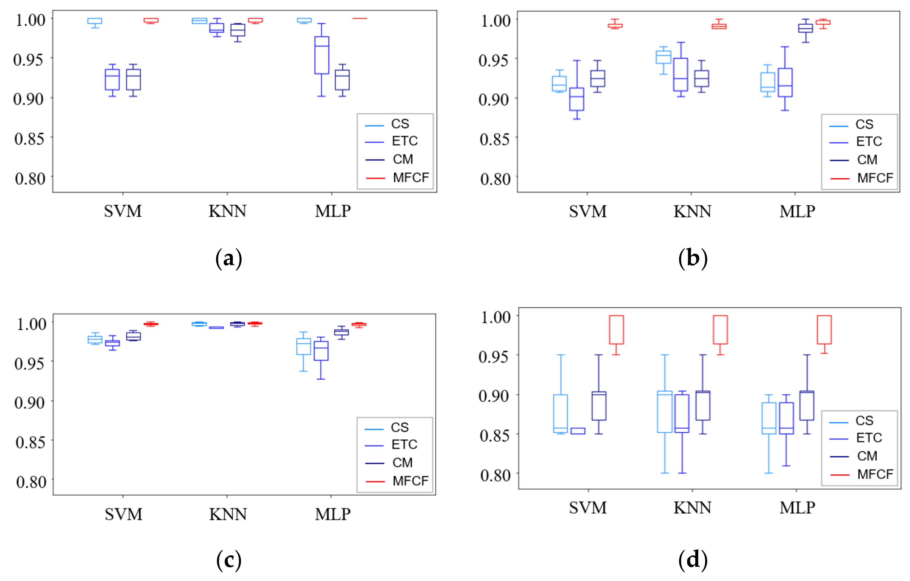
| Accuracy | CS | 0.93 | 0.99 | 0.93 | 0.91 | 0.95 | 0.92 | 0.97 | 0.99 | 0.96 | 0.76 | 0.94 | 0.95 | 0.93 |
| ETC | 0.98 | 0.99 | 0.96 | 0.88 | 0.95 | 0.93 | 0.98 | 0.99 | 0.97 | 0.86 | 0.99 | 0.96 | 0.95 | |
| CM | 0.93 | 0.98 | 0.93 | 0.93 | 0.97 | 0.98 | 0.98 | 0.99 | 0.98 | 0.94 | 0.98 | 0.96 | 0.96 | |
| MFCF | 1.0 | 1.0 | 1.0 | 0.99 | 1.0 | 0.99 | 0.99 | 0.99 | 0.99 | 1.0 | 1.0 | 1.0 | 0.99 | |
| Efficiency (sec.) | CS | 3.52 | 114.9 | 54.2 | 6.75 | 104.2 | 47.62 | 90.2 | 659.5 | 80.94 | 0.4 | 30.3 | 11.4 | 100.3 |
| ETC | 3.01 | 115.4 | 23.9 | 5.23 | 103.6 | 52.7 | 84.1 | 678.9 | 70.89 | 0.4 | 30.8 | 13.4 | 98.5 | |
| CM | 3.5 | 118.6 | 43.3 | 4.99 | 100.9 | 36.6 | 86.5 | 680.8 | 69.27 | 0.4 | 30.5 | 9.1 | 98.7 | |
| MFCF | 2.4 | 113.2 | 13.8 | 4.02 | 100.1 | 39.6 | 83.0 | 655.3 | 81.63 | 0.4 | 30.0 | 10.0 | 94.4 | |
Publisher’s Note: MDPI stays neutral with regard to jurisdictional claims in published maps and institutional affiliations. |
© 2022 by the authors. Licensee MDPI, Basel, Switzerland. This article is an open access article distributed under the terms and conditions of the Creative Commons Attribution (CC BY) license (https://creativecommons.org/licenses/by/4.0/).
Share and Cite
Mochammad, S.; Noh, Y.; Kang, Y.-J.; Park, S.; Lee, J.; Chin, S. Multi-Filter Clustering Fusion for Feature Selection in Rotating Machinery Fault Classification. Sensors 2022, 22, 2192. https://doi.org/10.3390/s22062192
Mochammad S, Noh Y, Kang Y-J, Park S, Lee J, Chin S. Multi-Filter Clustering Fusion for Feature Selection in Rotating Machinery Fault Classification. Sensors. 2022; 22(6):2192. https://doi.org/10.3390/s22062192
Chicago/Turabian StyleMochammad, Solichin, Yoojeong Noh, Young-Jin Kang, Sunhwa Park, Jangwoo Lee, and Simon Chin. 2022. "Multi-Filter Clustering Fusion for Feature Selection in Rotating Machinery Fault Classification" Sensors 22, no. 6: 2192. https://doi.org/10.3390/s22062192