
Combined Use of Cointegration Analysis and Robust Outlier Statistics to Improve Damage Detection in Real-World Structures


Abstract
:1. Introduction
2. Robust Outlier Detection
2.1. Minimum Covariance Determinant (MCD)
2.2. Threshold Estimation Based on Extreme Value Statistics
- A matrix is created ( is the number of dimensions and the number of observations), where each -dimensional observation is generated from a normal distribution, having zero mean and unit standard deviation.
- The desired discordancy measure (i.e., MSD or MCD) is calculated for all the observations, where mean and covariance are estimated depending on the selected classical or robust methods. The largest value for each matrix is stored.
- The process is repeated for a large number of iterations in order to create a vector of extreme distances. Then, all the values are sorted in decreasing order. The threshold value depends on the choice of the critical values . In the following analysis, is set equal to 5 per cent, giving a 95 per cent confidence limit.
3. Cointegration Basics
3.1. Order of Integration and Unit Root Tests
3.2. Linear Cointegration
3.3. Main Steps to Run Cointegration within SHM Applications
- Select a set of suitable monitored variables belonging to the same process and sharing common trends.
- Run the ADF test on the variables to determine the order of integration (this should be the same for all the variables).
- Split the original data set in two parts, one for training and one for testing. Training data are used to estimate the regression model, while test data are used to check for variations in system behaviour. To obtain a reliable model, training data should not include any damaged conditions, but should include a comprehensive time span and resolution of healthy data under different environmental and operational conditions.
- Run the ADF test on the model residual to assess its stationarity. If this situation is verified, the linear cointegrating relationship is successfully established and common trends are removed. Then, the cointegration residual represents a good indicator of the health status of the structure and can be used for damage detection purposes.
4. Proposed Hybrid Approach for Outlier Discrimination
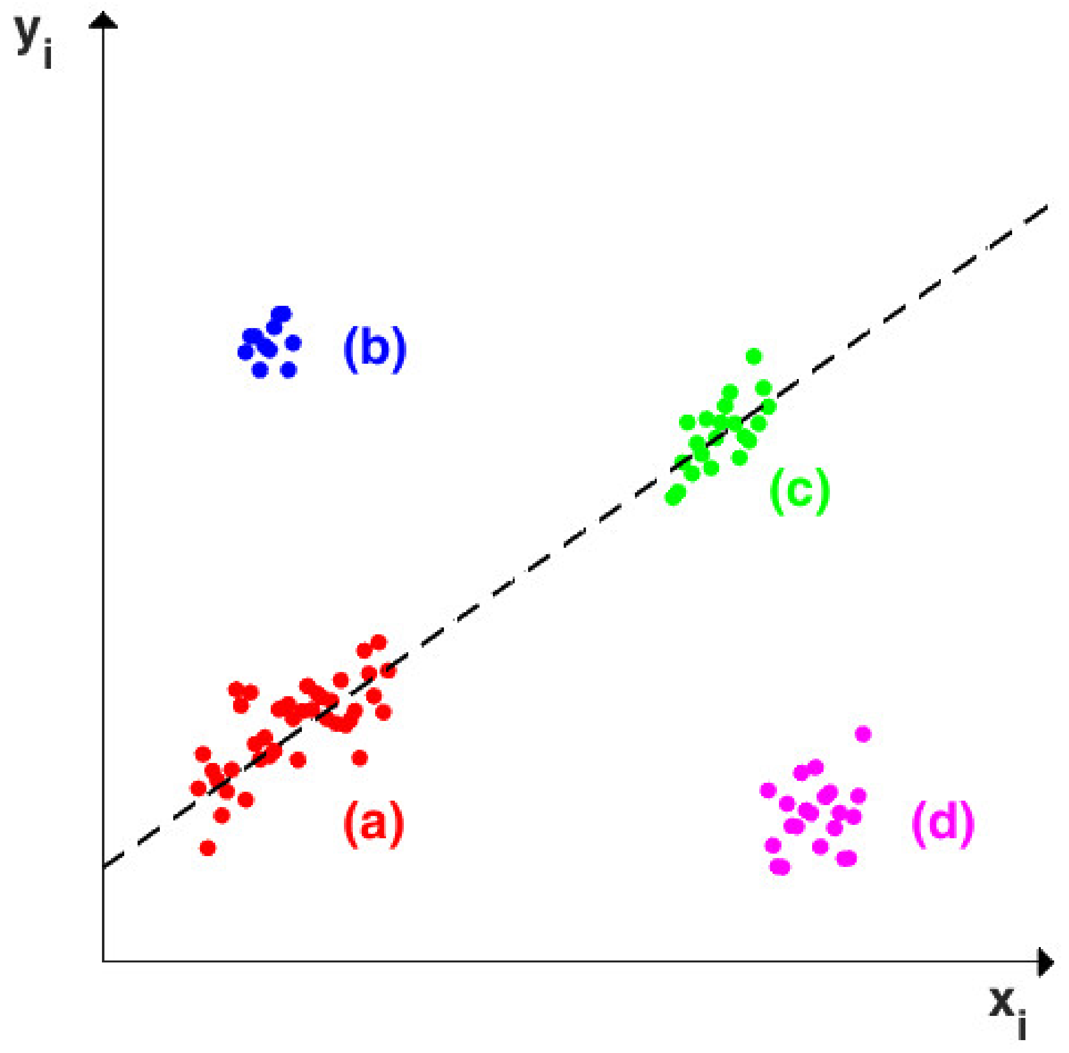
4.1. Identify Leverage Points in Regression
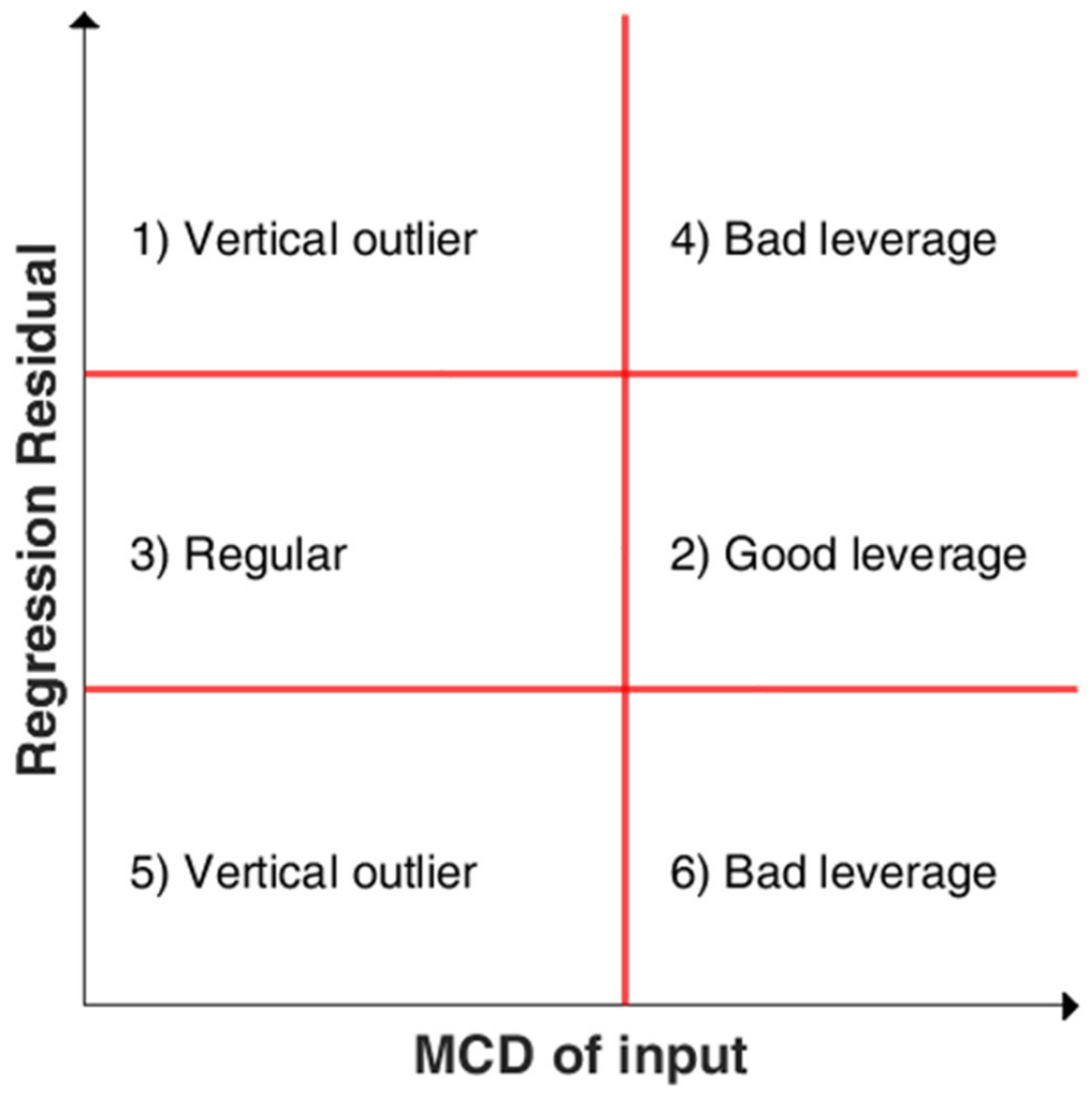
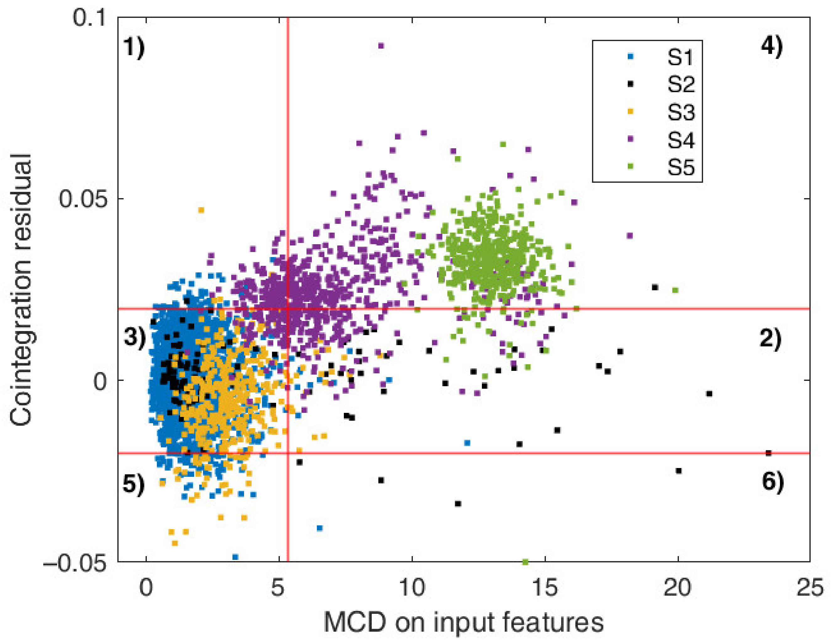
4.2. Description of the Residual Outlier Map
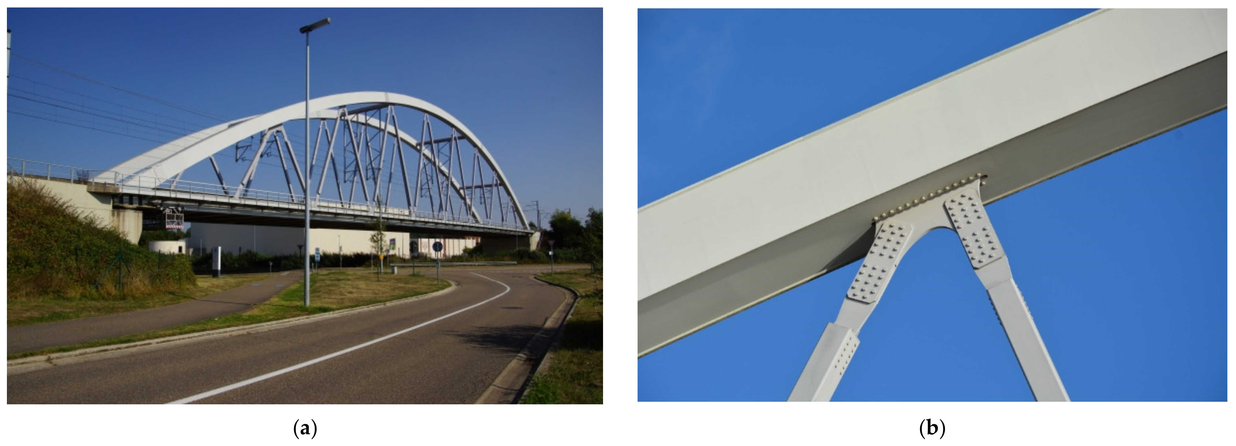
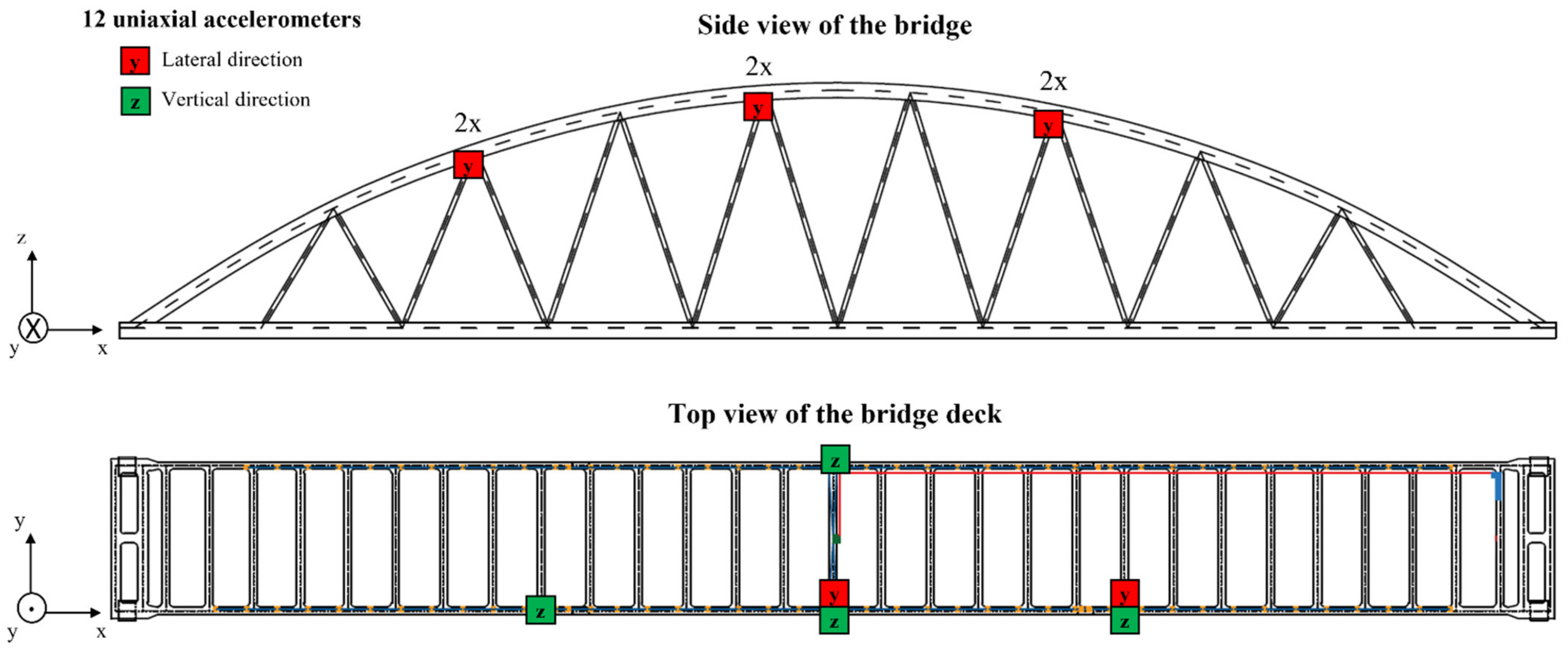
5. Application to SHM: The Railway Bridge KW51
6. Results and Discussions
7. Conclusions
Author Contributions
Funding
Institutional Review Board Statement
Informed Consent Statement
Data Availability Statement
Acknowledgments
Conflicts of Interest
Nomenclature
| Symbol/Abbreviation | Description |
| MSD | Mahalnobis squared distance |
| MCD | Minimum covariance determinant |
| zi | Multivariate observation |
| μz,Σ | Sample mean and covariance matrix |
| n | Number of samples |
| p | Number of features |
| [Z] | Multivariate feature matrix () |
| h | Breakdown value () |
| Hi | Subset of () |
| μi,Σi | Sample mean and covariance for data in |
| di(i) | MCD distance measure |
| ADF | Augmented Dickey–Fuller |
| yt | Generic time series |
| yt~I(d) | The time series is integrated of order |
| tρ | ADF t-statistic |
| EG | Engle-Granger |
| b = (1, −b2, …, −bn) | Cointegrating vector |
| εt | Cointegration residual |
| xi | -dimensional vector of predictors |
| yi | One-dimensional vector of the response |
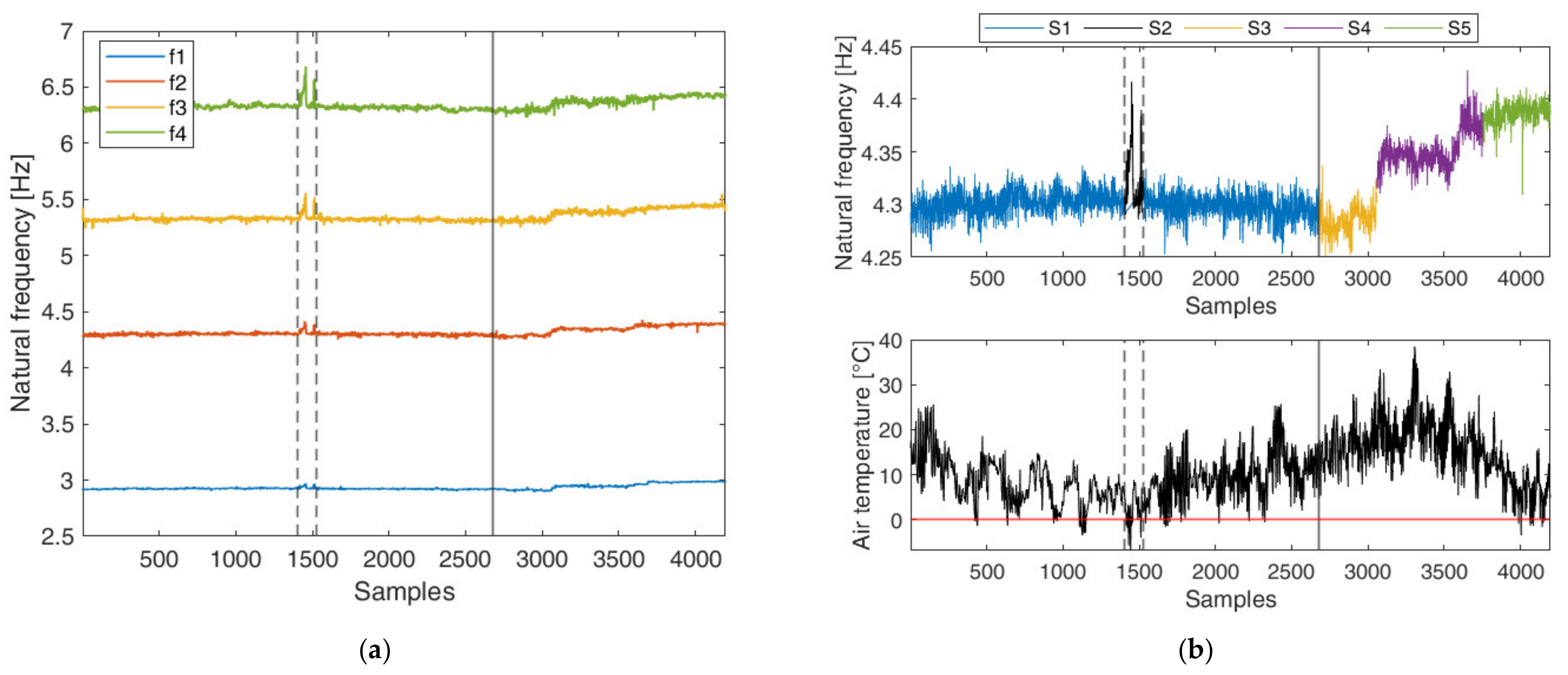
| f1,f2,f3,f4 | Natural frequencies of the KW51 bridge deck (vertical modes) |
References
- Gardner, P.; Fuentes, R.; Dervilis, N.; Mineo, C.; Pierce, S.G.; Cross, E.J.; Worden, K. Machine learning at the interface of structural health monitoring and non-destructive evaluation. Philos. Trans. R. Soc. A Math. Phys. Eng. Sci. 2020, 378, 20190581. [Google Scholar] [CrossRef]
- Hu, W.-H.; Tang, D.-H.; Teng, J.; Said, S.; Rohrmann, R.G. Structural Health Monitoring of a Prestressed Concrete Bridge Based on Statistical Pattern Recognition of Continuous Dynamic Measurements Over 14 Years. Sensors 2018, 18, 4117. [Google Scholar] [CrossRef] [PubMed] [Green Version]
- Pimentel, M.A.F.; Clifton, D.A.; Clifton, L.; Tarassenko, L. A review of novelty detection. Signal Process. 2014, 99, 215–249. [Google Scholar] [CrossRef]
- Worden, K.; Manson, G.; Fieller, N.R.J. Damage detection using outlier analysis. J. Sound Vib. 2000, 229, 647–667. [Google Scholar] [CrossRef]
- Ulriksen, M.D.; Damkilde, L. Structural damage localization by outlier analysis of signal-processed mode shapes—Analytical and experimental validation. Mech. Syst. Signal Process. 2016, 68–69, 1–14. [Google Scholar] [CrossRef]
- Worden, K. Structural fault detection using a novelty measure. J. Sound Vib. 1997, 201, 85–101. [Google Scholar] [CrossRef]
- Mahalanobis, P.C. On the Generalized Distance in Statistics; National Institute of Science of India: Calcutta, India, 1936; pp. 49–55. [Google Scholar]
- Turrisi, S.; Zappa, E.; Cigada, A.; Vivanco, M.R.; Avin, N.C. Effect of image acquisition and processing parameters on the estimation of crowd-induced dynamic loading on stadium grandstands. In Proceedings of the 2021 IEEE International Instrumentation and Measurement Technology Conference (I2MTC), Glasgow, UK, 17–20 May 2021. [Google Scholar]
- Wang, X.; Gao, Q.; Liu, Y. Damage Detection of Bridges under Environmental Temperature Changes Using a Hybrid Method. Sensors 2020, 20, 3999. [Google Scholar] [CrossRef]
- An, Y.; Chatzi, E.; Sim, S.; Laflamme, S.; Blachowski, B.; Ou, J. Recent progress and future trends on damage identification methods for bridge structures. Struct. Control Health Monit. 2019, 26, e2416. [Google Scholar] [CrossRef]
- Cai, Y.; Zhang, K.; Ye, Z.; Liu, C.; Lu, K.; Wang, L. Influence of Temperature on the Natural Vibration Characteristics of Simply Supported Reinforced Concrete Beam. Sensors 2021, 21, 4242. [Google Scholar] [CrossRef]
- Teng, J.; Tang, D.-H.; Zhang, X.; Hu, W.-H.; Said, S.; Rohrmann, R. Automated Modal Analysis for Tracking Structural Change during Construction and Operation Phases. Sensors 2019, 19, 927. [Google Scholar] [CrossRef] [Green Version]
- Dervilis, N.; Cross, E.J.; Barthorpe, R.J.; Worden, K. Robust methods of inclusive outlier analysis for structural health monitoring. J. Sound Vib. 2014, 333, 5181–5195. [Google Scholar] [CrossRef]
- Yeager, M.; Gregory, B.; Key, C.; Todd, M. On using robust Mahalanobis distance estimations for feature discrimination in a damage detection scenario. Struct. Health Monit. 2019, 18, 245–253. [Google Scholar] [CrossRef]
- Fuentes, R.; Gardner, P.; Mineo, C.; Rogers, T.J.; Pierce, S.G.; Worden, K.; Dervilis, N.; Cross, E.J. Autonomous ultrasonic inspection using Bayesian optimisation and robust outlier analysis. Mech. Syst. Signal Process. 2020, 145, 106897. [Google Scholar] [CrossRef]
- Rosafalco, L.; Manzoni, A.; Mariani, S.; Corigliano, A. An Autoencoder-Based Deep Learning Approach for Load Identification in Structural Dynamics. Sensors 2021, 21, 4207. [Google Scholar] [CrossRef]
- Sohn, H. Effects of environmental and operational variability on structural health monitoring. Philos. Trans. R. Soc. A Math. Phys. Eng. Sci. 2007, 365, 539–560. [Google Scholar] [CrossRef]
- Deraemaeker, A.; Worden, K. A comparison of linear approaches to filter out environmental effects in structural health monitoring. Mech. Syst. Signal Process. 2018, 105, 1–15. [Google Scholar] [CrossRef]
- Yan, A.M.; Kerschen, G.; De Boe, P.; Golinval, J.C. Structural damage diagnosis under varying environmental conditions—Part I: A linear analysis. Mech. Syst. Signal Process. 2005, 19, 847–864. [Google Scholar] [CrossRef]
- Svendsen, B.T.; Frøseth, G.T.; Øiseth, O.; Rønnquist, A. A data-based structural health monitoring approach for damage detection in steel bridges using experimental data. J. Civ. Struct. Health Monit. 2021, 12, 101–115. [Google Scholar] [CrossRef]
- Cross, E.J.; Worden, K.; Chen, Q. Cointegration: A novel approach for the removal of environmental trends in structural health monitoring data. Proc. R. Soc. A Math. Phys. Eng. Sci. 2011, 467, 2712–2732. [Google Scholar] [CrossRef]
- Rytter, A. Vibrational Based Inspection of Civil Engineering Structures. Ph.D. Thesis, Aalborg University, Aalborg, Denmark, 1993. [Google Scholar]
- Frigui, F.; Faye, J.P.; Martin, C.; Dalverny, O.; Peres, F.; Judenherc, S. Global methodology for damage detection and localization in civil engineering structures. Eng. Struct. 2018, 171, 686–695. [Google Scholar] [CrossRef] [Green Version]
- Turrisi, S.; Cigada, A.; Zappa, E. A cointegration-based approach for automatic anomalies detection in large-scale structures. Mech. Syst. Signal Process. 2022, 166, 108483. [Google Scholar] [CrossRef]
- Salvetti, M.; Sbarufatti, C.; Cross, E.; Corbetta, M.; Worden, K.; Giglio, M. On the performance of a cointegration-based approach for novelty detection in realistic fatigue crack growth scenarios. Mech. Syst. Signal Process. 2019, 123, 84–101. [Google Scholar] [CrossRef] [Green Version]
- Sousa Tomé, E.; Pimentel, M.; Figueiras, J. Damage detection under environmental and operational effects using cointegration analysis—Application to experimental data from a cable-stayed bridge. Mech. Syst. Signal Process. 2020, 135, 106386. [Google Scholar] [CrossRef]
- Liang, Y.; Li, D.; Song, G.; Feng, Q. Frequency Co-integration-based damage detection for bridges under the influence of environmental temperature variation. Measurement 2018, 125, 163–175. [Google Scholar] [CrossRef]
- Coletta, G.; Miraglia, G.; Pecorelli, M.; Ceravolo, R.; Cross, E.; Surace, C.; Worden, K. Use of the cointegration strategies to remove environmental effects from data acquired on historical buildings. Eng. Struct. 2019, 183, 1014–1026. [Google Scholar] [CrossRef]
- Dervilis, N.; Worden, K.; Cross, E.J. On robust regression analysis as a means of exploring environmental and operational conditions for SHM data. J. Sound Vib. 2015, 347, 279–296. [Google Scholar] [CrossRef] [Green Version]
- Magalhães, F.; Cunha, A.; Caetano, E. Vibration based structural health monitoring of an arch bridge: From automated OMA to damage detection. Mech. Syst. Signal Process. 2012, 28, 212–228. [Google Scholar] [CrossRef]
- Pereira, S.; Magalhães, F.; Gomes, J.P.; Cunha, Á.; Lemos, J.V. Vibration-based damage detection of a concrete arch dam. Eng. Struct. 2021, 235, 112032. [Google Scholar] [CrossRef]
- Johnson, E.A.; Lam, H.F.; Katafygiotis, L.S.; Beck, J.L. Phase I IASC-ASCE Structural Health Monitoring Benchmark Problem Using Simulated Data. J. Eng. Mech. 2004, 130, 3–15. [Google Scholar] [CrossRef]
- Shi, H.; Worden, K.; Cross, E.J. A nonlinear cointegration approach with applications to structural health monitoring. J. Phys. Conf. Ser. 2016, 744. [Google Scholar] [CrossRef]
- Peeters, B.; De Roeck, G. One-year monitoring of the Z24-bridge: Environmental effectsversus damage events. Earthq. Eng. Struct. Dyn. 2001, 30, 149–171. [Google Scholar] [CrossRef]
- Langone, R.; Reynders, E.; Mehrkanoon, S.; Suykens, J.A.K. Automated structural health monitoring based on adaptive kernel spectral clustering. Mech. Syst. Signal Process. 2017, 90, 64–78. [Google Scholar] [CrossRef] [Green Version]
- Maes, K.; Lombaert, G. Monitoring data for railway bridge KW51 in Leuven, Belgium, before, during, and after retrofitting. J. Bridge Eng. 2021, 26, 04721001. [Google Scholar] [CrossRef]
- Turrisi, S.; Zappa, E.; Cigada, A.; Hötzer, T. Large structures natural frequencies estimation using a limited number of sensors. In Proceedings of the 2020 IEEE International Instrumentation and Measurement Technology Conference (I2MTC), Dubrovnik, Croatia, 25–28 May 2020; pp. 1–6. [Google Scholar]
- Anastasopoulos, D.; De Roeck, G.; Reynders, E.P.B. One-year operational modal analysis of a steel bridge from high-resolution macrostrain monitoring: Influence of temperature vs. retrofitting. Mech. Syst. Signal Process. 2021, 161, 107951. [Google Scholar] [CrossRef]
- Maes, K.; Van Meerbeeck, L.; Reynders, E.P.B.; Lombaert, G. Validation of vibration-based structural health monitoring on retrofitted railway bridge KW51. Mech. Syst. Signal Process. 2022, 165, 108380. [Google Scholar] [CrossRef]
- Gnanadesikan, R.; Kettenring, J.R. Robust Estimates, Residuals, and Outlier Detection with Multiresponse Data. Biometrics 1972, 28, 81. [Google Scholar] [CrossRef]
- Rousseeuw, P.J. Least Median of Squares Regression. J. Am. Stat. Assoc. 1984, 79, 871–880. [Google Scholar] [CrossRef]
- Rousseeuw, P.; Leroy, A. Robust Regression and Outlier Detection; John Wiley and Sons: New York, NY, USA, 2005; Volume 589. [Google Scholar]
- Maronna, R.A.; Zamar, R.H. Robust Estimates of Location and Dispersion for High-Dimensional Datasets. Technometrics 2002, 44, 307–317. [Google Scholar] [CrossRef]
- Maronna, R.A. Robust Estimators of Multivariate Location and Scatter. Ann. Stat. 1976, 4, 51–67. [Google Scholar] [CrossRef]
- Rousseeuw, P.J.; Driessen, K.V. A Fast Algorithm for the Minimum Covariance Determinant Estimator. Technometrics 1999, 41, 212–223. [Google Scholar] [CrossRef]
- Verboven, S.; Hubert, M. LIBRA: A matlab library for robust analysis. Chemom. Intell. Lab. Syst. 2005, 75, 127–136. [Google Scholar] [CrossRef]
- Srinivasa Rao, P.; Ratnam, C. Health monitoring of welded structures using statistical process control. Mech. Syst. Signal Process. 2012, 27, 683–695. [Google Scholar] [CrossRef]
- Zapico-Valle, J.L.; García-Diéguez, M.; González-Martínez, M.P.; Worden, K. Experimental validation of a new statistical process control feature for damage detection. Mech. Syst. Signal Process. 2011, 25, 2513–2525. [Google Scholar] [CrossRef]
- Said, S.E.; Dickey, D.A. Testing for unit roots in autoregressive-moving average models of unknown order. Biometrika 1984, 71, 599–607. [Google Scholar] [CrossRef]
- Johansen, S. Statistical analysis of cointegration vectors. J. Econ. Dyn. Control 1988, 12, 231–254. [Google Scholar] [CrossRef]
- Engle, R.F.; Granger, C.W.J. Co-integration and error correction: Representation, estimation, and testing. Appl. Econom. 2015, 39, 106–135. [Google Scholar]
- Li, F.; Wang, Z.; Liu, G. Towards an Error Correction Model for dam monitoring data analysis based on Cointegration Theory. Struct. Saf. 2013, 43, 12–20. [Google Scholar] [CrossRef]
- Hubert, M.; Rousseeuw, P.J.; Van Aelst, S. High-Breakdown Robust Multivariate Methods. Stat. Sci. 2008, 23, 92–119. [Google Scholar] [CrossRef]
- Anastasopoulos, D. Structural Health Monitoring Based on Operational Modal Analysis from Long Gauge Dynamic Strain Measurements. Ph.D. Thesis, KU Leuven, Leuven, Belgium, 2020. [Google Scholar]
- Moser, P.; Moaveni, B. Environmental effects on the identified natural frequencies of the Dowling Hall Footbridge. Mech. Syst. Signal Process. 2011, 25, 2336–2357. [Google Scholar] [CrossRef]


| Scenario | Description | Data Points |
|---|---|---|
| S1 | Before retrofitting | 1–1403; 1531–2674 |
| S2 | Before retrofitting (cold temperatures) | 1404–1530 |
| S3 | Retrofitting: 1st stage | 2675–3058 |
| S4 | Retrofitting: 2nd stage | 3059–3755 |
| S5 | Post retrofitting | 3756–4196 |
| Variables | ADF t-Statistic | 5% Critical Value | Stationarity? |
|---|---|---|---|
| 0.041 | −1.942 | NO | |
| 0.030 | −1.942 | NO | |
| −0.091 | −1.942 | NO | |
| −0.072 | −1.942 | NO |
| Variables | ADF t-Statistic | 5% Critical Value | Stationarity? |
|---|---|---|---|
| −14.491 | −1.942 | Y | |
| −18.629 | −1.942 | Y | |
| −17.557 | −1.942 | Y | |
| −12.301 | −1.942 | Y |
Publisher’s Note: MDPI stays neutral with regard to jurisdictional claims in published maps and institutional affiliations. |
© 2022 by the authors. Licensee MDPI, Basel, Switzerland. This article is an open access article distributed under the terms and conditions of the Creative Commons Attribution (CC BY) license (https://creativecommons.org/licenses/by/4.0/).
Share and Cite
Turrisi, S.; Zappa, E.; Cigada, A. Combined Use of Cointegration Analysis and Robust Outlier Statistics to Improve Damage Detection in Real-World Structures. Sensors 2022, 22, 2177. https://doi.org/10.3390/s22062177
Turrisi S, Zappa E, Cigada A. Combined Use of Cointegration Analysis and Robust Outlier Statistics to Improve Damage Detection in Real-World Structures. Sensors. 2022; 22(6):2177. https://doi.org/10.3390/s22062177
Chicago/Turabian StyleTurrisi, Simone, Emanuele Zappa, and Alfredo Cigada. 2022. "Combined Use of Cointegration Analysis and Robust Outlier Statistics to Improve Damage Detection in Real-World Structures" Sensors 22, no. 6: 2177. https://doi.org/10.3390/s22062177