
No-Reference Quality Assessment of Stereoscopic Video Based on Temporal Adaptive Model for Improved Visual Communication
Abstract
:1. Introduction
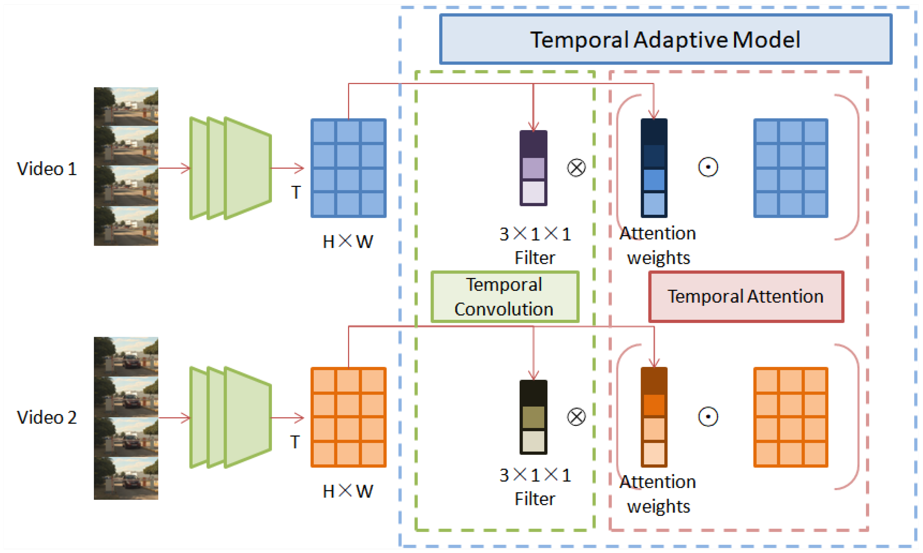
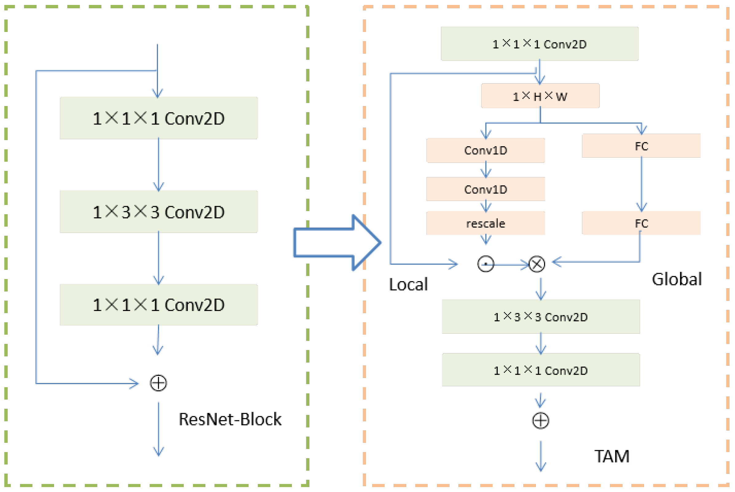
- Temporal modeling is the key to capture spatiotemporal distortion in video. Affected by camera motion, speed changes and other factors, video data have extremely complex dynamics in the time dimension. In order to effectively capture such diverse motion patterns, a temporal adaptive module (TAM) is proposed, which generates a video-specific kernel based on its own feature mapping. The TAM can learn and obtain short-term information from the local time window. This information is generated from the global view, and it pays more attention to long-term goals.
- The framework describes video frames from two parts: local short-term relation and global relation. This model can be flexibly embedded into any 2D CNN framework and can still use the pretrained backbone network parameters without significantly increasing the complexity of the model.
- Rich performance verification experiments are performed. From the results, the prediction of this model is in good agreement with the subjective quality. Moreover, compared with existing methods, the proposed method has a higher visual quality perception prediction accuracy in both symmetric and asymmetric distortion databases.
2. Related Works
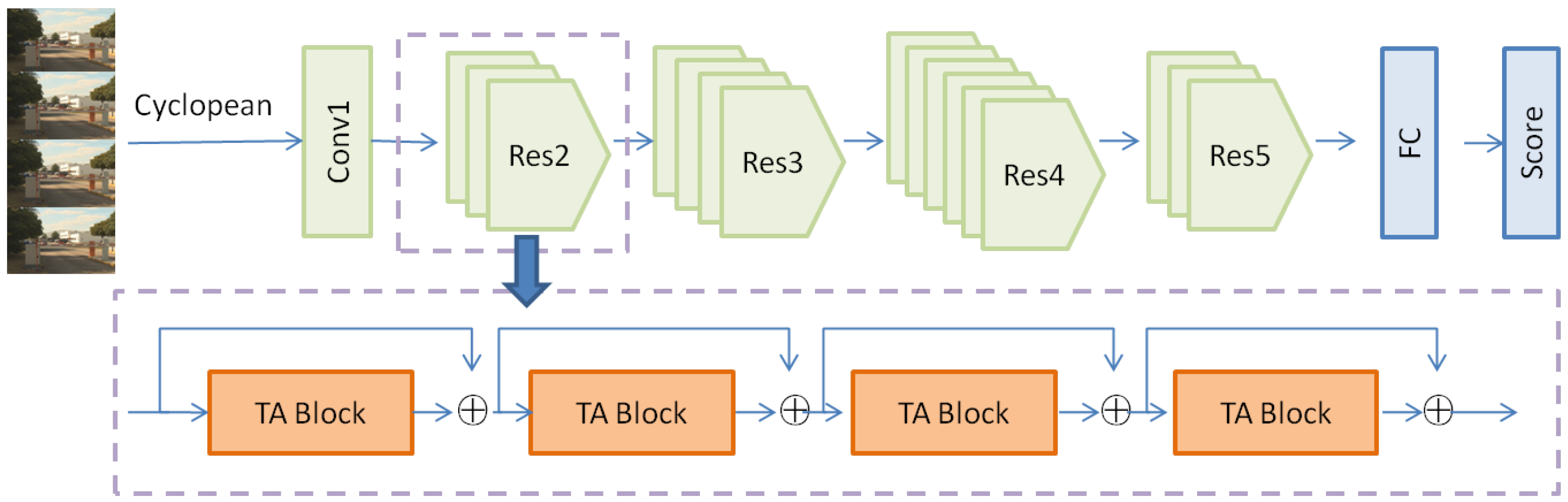
3. Method of SVQA
3.1. Stereoscopic Formation
3.2. Temporal Adaptive Module
3.3. Objective Quality Score Estimation
4. Experiments
4.1. Databases and Indicators
4.2. Overall Performance
4.3. Experiments under Different Distortion Types
4.4. Ablation Experiment
5. Conclusions
Author Contributions
Funding
Institutional Review Board Statement
Informed Consent Statement
Data Availability Statement
Acknowledgments
Conflicts of Interest
References
- Xu, N.; Fang, X.; Li, W.; An, Y. Perception-based Asymmetric Video Coding for 3D Video. In Proceedings of the 2020 IEEE 2nd International Conference on Civil Aviation Safety and Information Technology (ICCASIT), Weihai, China, 14–16 October 2020. [Google Scholar]
- Hou, Y.; Liu, L.; Zhang, Y.; Sang, Q. Stereoscopic Video Quality Assessment Using Oriented Local Gravitational Force Statistics. IEEE Access 2020, 8, 212442–212455. [Google Scholar] [CrossRef]
- Jin, Y.; Chen, M.; Goodall, T.; Patney, A.; Bovik, A.C. Subjective and Objective Quality Assessment of 2D and 3D Foveated Video Compression in Virtual Reality. IEEE Trans. Image Process. 2021, 30, 5905–5919. [Google Scholar] [CrossRef] [PubMed]
- Feng, Y.; Li, S.; Chang, Y. Multi-Scale Feature-Guided Stereoscopic Video Quality Assessment Based on 3d Convolutional Neural Network. In Proceedings of the ICASSP 2021—2021 IEEE International Conference on Acoustics, Speech and Signal Processing (ICASSP), Toronto, ON, Canada, 6–11 June 2021. [Google Scholar] [CrossRef]
- Appina, B.; Sharma, M.; Kumar, S.; Kara, P.A.; Simon, A.; Guindy, M. Latent Factor Modeling of Perceived Quality for Stereoscopic 3D Video Recommendation. In Proceedings of the 2021 International Conference on 3D Immersion (IC3D), Brussels, Belgium, 8 December 2021. [Google Scholar] [CrossRef]
- Wang, J.; Wang, S.; Wang, Z. Asymmetrically Compressed Stereoscopic 3D Videos: Quality Assessment and Rate-Distortion Performance Evaluation. IEEE Trans. Image Process. 2017, 26, 1330–1343. [Google Scholar] [CrossRef] [PubMed]
- Wan, W.; Huang, D.; Shang, B.; Wei, S.; Wu, H.R.; Wu, J.; Shi, G. Depth Perception Assessment of 3D Videos Based on Stereoscopic and Spatial Orientation Structural Features. IEEE Trans. Circuits Syst. Video Technol. 2022. [Google Scholar] [CrossRef]
- Yang, J.; Zhu, Y.; Ma, C.; Lu, W.; Meng, Q. Stereoscopic video quality assessment based on 3D convolutional neural networks. Neurocomputing 2018, 309, 83–93. [Google Scholar] [CrossRef] [Green Version]
- Imani, H.; Islam, M.B.; Arica, N. Three-Stream 3D deep CNN for no-Reference stereoscopic video quality assessment. Intell. Syst. Appl. 2022, 13, 200059. [Google Scholar] [CrossRef]
- Feng, Y.; Li, S. Stereoscopic Video Quality Assessment with Multi-level Binocular Fusion Network Considering Disparity and Multi-scale Information. In Proceedings of the 2021 International Conference on Visual Communications and Image Processing (VCIP), Munich, Germany, 5–8 December 2021. [Google Scholar] [CrossRef]
- Li, Y.; Yang, J.; Zhang, Z.; Wen, J.; Kumar, P. Healthcare Data Quality Assessment for Cybersecurity Intelligence. IEEE Trans. Ind. Inform. 2022. [Google Scholar] [CrossRef]
- Pinson, M.; Wolf, S. A New Standardized Method for Objectively Measuring Video Quality. IEEE Trans. Broadcast. 2004, 50, 312–322. [Google Scholar] [CrossRef]
- Hewage, C.; Worrall, S.; Dogan, S.; Kondoz, A. Prediction of stereoscopic video quality using objective quality models of 2-D video. Electron. Lett. 2008, 44, 963. [Google Scholar] [CrossRef] [Green Version]
- Chen, M.J.; Kwon, D.K.; Bovik, A.C. Study of subject agreement on stereoscopic video quality. In Proceedings of the 2012 IEEE Southwest Symposium on Image Analysis and Interpretation, Santa Fe, NM, USA, 22–24 April 2012. [Google Scholar] [CrossRef] [Green Version]
- Fang, Y.; Sui, X.; Wang, J.; Yan, J.; Lei, J.; Callet, P.L. Perceptual Quality Assessment for Asymmetrically Distorted Stereoscopic Video by Temporal Binocular Rivalry. IEEE Trans. Circuits Syst. Video Technol. 2021, 31, 3010–3024. [Google Scholar] [CrossRef]
- Galkandage, C.; Calic, J.; Dogan, S.; Guillemaut, J.Y. Stereoscopic Video Quality Assessment Using Binocular Energy. IEEE J. Sel. Top. Signal Process. 2017, 11, 102–112. [Google Scholar] [CrossRef] [Green Version]
- Appina, B.; Dendi, S.V.R.; Manasa, K.; Channappayya, S.S.; Bovik, A.C. Study of Subjective Quality and Objective Blind Quality Prediction of Stereoscopic Videos. IEEE Trans. Image Process. 2019, 28, 5027–5040. [Google Scholar] [CrossRef]
- Jin, L.; Boev, A.; Gotchev, A.; Egiazarian, K. 3D-DCT based perceptual quality assessment of stereo video. In Proceedings of the 2011 18th IEEE International Conference on Image Processing, Brussels, Belgium, 11–14 September 2011. [Google Scholar] [CrossRef]
- Liu, Z.; Wang, L.; Wu, W.; Qian, C.; Lu, T. TAM: Temporal Adaptive Module for Video Recognition. In Proceedings of the 2021 IEEE/CVF International Conference on Computer Vision (ICCV), Montreal, QC, Canada, 10–17 October 2021. [Google Scholar] [CrossRef]
- Qi, F.; Jiang, T.; Fan, X.; Ma, S.; Zhao, D. Stereoscopic video quality assessment based on stereo just-noticeable difference model. In Proceedings of the 2013 IEEE International Conference on Image Processing, Melbourne, Australia, 15–18 September 2013. [Google Scholar] [CrossRef]
- Urvoy, M.; Barkowsky, M.; Cousseau, R.; Koudota, Y.; Ricorde, V.; Callet, P.L.; Gutierrez, J.; Garcia, N. NAMA3DS1-COSPAD1: Subjective video quality assessment database on coding conditions introducing freely available high quality 3D stereoscopic sequences. In Proceedings of the 2012 Fourth International Workshop on Quality of Multimedia Experience, Melbourne, Australia, 5–7 July 2012. [Google Scholar] [CrossRef]
- Wang, J.; Wang, S.; Wang, Z. Quality prediction of asymmetrically compressed stereoscopic videos. In Proceedings of the 2015 IEEE International Conference on Image Processing (ICIP), Quebec City, QC, Canada, 27–30 September 2015. [Google Scholar] [CrossRef]
- Zhang, Y.; Liu, X.; Liu, H.; Fan, C. Depth perceptual quality assessment for symmetrically and asymmetrically distorted stereoscopic 3D videos. Signal Process. Image Commun. 2019, 78, 293–305. [Google Scholar] [CrossRef]
- Imani, H.; Islam, M.B.; Wong, L.K. A New Dataset and Transformer for Stereoscopic Video Super-Resolution. In Proceedings of the 2022 IEEE/CVF Conference on Computer Vision and Pattern Recognition Workshops (CVPRW), New Orleans, LA, USA, 19–20 June 2022; pp. 705–714. [Google Scholar] [CrossRef]
- Galkandage, C.; Calic, J.; Dogan, S.; Guillemaut, J.Y. Full-Reference Stereoscopic Video Quality Assessment Using a Motion Sensitive HVS Model. IEEE Trans. Circuits Syst. Video Technol. 2021, 31, 452–466. [Google Scholar] [CrossRef] [Green Version]
- Liu, L.; Wang, T.; Huang, H. Pre-Attention and Spatial Dependency Driven No-Reference Image Quality Assessment. IEEE Trans. Multimed. 2019, 21, 2305–2318. [Google Scholar] [CrossRef]
- Wang, Z.; Bovik, A.; Sheikh, H.; Simoncelli, E. Image Quality Assessment: From Error Visibility to Structural Similarity. IEEE Trans. Image Process. 2004, 13, 600–612. [Google Scholar] [CrossRef] [Green Version]
- Wang, Z.; Simoncelli, E.; Bovik, A. Multiscale structural similarity for image quality assessment. In Proceedings of the The Thrity-Seventh Asilomar Conference on Signals, Systems & Computers, Pacific Grove, CA, USA, 9–12 November 2003. [Google Scholar] [CrossRef] [Green Version]
- Mittal, A.; Moorthy, A.K.; Bovik, A.C. No-Reference Image Quality Assessment in the Spatial Domain. IEEE Trans. Image Process. 2012, 21, 4695–4708. [Google Scholar] [CrossRef]
- Qi, F.; Zhao, D.; Fan, X.; Jiang, T. Stereoscopic video quality assessment based on visual attention and just-noticeable difference models. Signal, Image Video Process. 2015, 10, 737–744. [Google Scholar] [CrossRef]
- Chen, Z.; Zhou, W.; Li, W. Blind Stereoscopic Video Quality Assessment: From Depth Perception to Overall Experience. IEEE Trans. Image Process. 2018, 27, 721–734. [Google Scholar] [CrossRef]
- Appina, B.; Channappayya, S.S. Full-Reference 3-D Video Quality Assessment Using Scene Component Statistical Dependencies. IEEE Signal Process. Lett. 2018, 25, 823–827. [Google Scholar] [CrossRef]
- Silva, V.D.; Arachchi, H.K.; Ekmekcioglu, E.; Kondoz, A. Toward an Impairment Metric for Stereoscopic Video: A Full-Reference Video Quality Metric to Assess Compressed Stereoscopic Video. IEEE Trans. Image Process. 2013, 22, 3392–3404. [Google Scholar] [CrossRef] [PubMed]
- Jiang, G.; Liu, S.; Yu, M.; Shao, F.; Peng, Z.; Chen, F. No reference stereo video quality assessment based on motion feature in tensor decomposition domain. J. Vis. Commun. Image Represent. 2018, 50, 247–262. [Google Scholar] [CrossRef]


| Category | FR | NR | ||||||
|---|---|---|---|---|---|---|---|---|
| Method | PSNR | SSIM | MS-SSIM | SJND-SVA | BRISQUE | BSVQE | Ours | |
| H.264 | PLCC | 0.6595 | 0.8371 | 0.8401 | - | 0.8704 | 0.9371 | 0.9450 |
| SROCC | 0.8437 | 0.8566 | 0.8546 | - | 0.8446 | 0.9379 | 0.9334 | |
| RMSE | 0.74381 | 0.5413 | 0.5368 | - | 0.4791 | - | 0.3133 | |
| Blur | PLCC | 0.6933 | 0.8342 | 0.8576 | - | 0.8493 | 0.9568 | 0.9666 |
| SROCC | 0.8417 | 0.8420 | 0.8607 | - | 0.8306 | 0.9505 | 0.9563 | |
| RMSE | 0.7186 | 0.5498 | 0.5129 | - | 0.5202 | - | 0.2483 | |
| Overall | PLCC | 0.7223 | 0.8346 | 0.8472 | 0.8415 | 0.8525 | 0.9394 | 0.9520 |
| SROCC | 0.8361 | 0.8476 | 0.5567 | 0.8379 | 0.8448 | 0.9387 | 0.9458 | |
| RMSE | 0.6878 | 0.5478 | 0.5284 | 0.5372 | 0.5210 | - | 0.2994 | |
| Category | NR | |||||
|---|---|---|---|---|---|---|
| Method | PSNR | SSIM | DPDI | BSVQE | Ours | |
| H.264 | PLCC | 0.7043 | 0.6932 | 0.6862 | 0.8898 | 0.8914 |
| SROCC | 0.6228 | 0.6656 | 0.5982 | 0.8225 | 0.8310 | |
| RMSE | 0.5721 | 0.5807 | 0.5659 | 0.3537 | 0.3523 | |
| JPEG2000 | PLCC | 0.3900 | 0.5018 | 0.4311 | 0.6523 | 0.7611 |
| SROCC | 0.3156 | 0.2141 | 0.3196 | 0.5503 | 0.6611 | |
| RMSE | 0.3789 | 0.3559 | 0.3467 | 0.2888 | 0.2626 | |
| Overall | PLCC | 0.6414 | 0.6097 | 0.5660 | 0.8810 | 0.8862 |
| SROCC | 0.5197 | 0.5146 | 0.4858 | 0.8208 | 0.8271 | |
| RMSE | 0.5145 | 0.5315 | 0.5355 | 0.3074 | 0.3051 | |
| Category | FR | |||||||
|---|---|---|---|---|---|---|---|---|
| Method | PSNR | SSIM | MS-SSIM | SJND-SVA | StSD | DeMo_3D (MS-SSIM) | Ours | |
| H.264 | PLCC | 0.5758 | 0.7365 | 0.7885 | 0.5834 | 0.8020 | 0.9161 | 0.9541 |
| SROCC | 0.5425 | 0.7172 | 0.6673 | 0.6810 | 0.7575 | 0.9009 | 0.9441 | |
| RMSE | 0.9463 | 0.7953 | 0.6955 | 0.6672 | - | 0.4654 | 0.2523 | |
| JPEG2000 | PLCC | 0.8073 | 0.9290 | 0.9439 | 0.8062 | 0.8433 | 0.9505 | 0.9666 |
| SROCC | 0.7651 | 0.8879 | 0.9299 | 0.6901 | 0.8494 | 0.9326 | 0.9611 | |
| RMSE | 0.7362 | 0.4611 | 0.4327 | 0.8629 | - | 0.4074 | 0.1426 | |
| Overall | PLCC | 0.6667 | 0.7981 | 0.8506 | 0.6503 | 0.7978 | 0.9242 | 0.9562 |
| SROCC | 0.6230 | 0.7565 | 0.8534 | 0.6229 | 0.8162 | 0.9187 | 0.9471 | |
| RMSE | 0.8809 | 0.7121 | 0.5512 | 0.8629 | - | 0.4651 | 0.3151 | |
| Category | NR | ||||
|---|---|---|---|---|---|
| Method | MNSVQM | BRISQUE | BSVQE | Ours | |
| H.264 | PLCC | 0.8850 | 0.9329 | 0.9168 | 0.9541 |
| SROCC | 0.7714 | 0.8697 | 0.8857 | 0.9441 | |
| RMSE | 0.4675 | 0.3722 | - | 0.2523 | |
| JPEG2000 | PLCC | 0.9706 | 0.9055 | 0.8953 | 0.9666 |
| SROCC | 0.8982 | 0.8503 | 0.8383 | 0.9611 | |
| RMSE | 0.2769 | 0.4904 | - | 0.1426 | |
| Overall | PLCC | 0.8611 | 0.8897 | 0.9239 | 0.9562 |
| SROCC | 0.8394 | 0.8490 | 0.9086 | 0.9471 | |
| RMSE | 0.5634 | 0.5236 | - | 0.3151 | |
| WaterlooIVC 3D Video Phase I | ||||
|---|---|---|---|---|
| Category | Method | PLCC | SROCC | RMSE |
| FR | PSNR | 0.7085 | 0.5336 | 15.4507 |
| SSIM | 0.3964 | 0.2872 | 20.1010 | |
| MS-SSIM | 0.4072 | 0.2969 | 19.9978 | |
| StSD | 0.7880 | 0.7543 | - | |
| (MS-SSIM) | 0.8943 | 0.8806 | 9.4853 | |
| NR | BRISQUE | 0.8711 | 0.8416 | 10.3788 |
| BSVQE | 0.9343 | 0.8883 | 7.7882 | |
| Ours | 0.9347 | 0.9027 | 7.4165 | |
| Component | Ours w/o TAM | Ours w/o Global | Ours w/o Local | Ours | |
|---|---|---|---|---|---|
| NAMA3DS1-COSPAD1 | PLCC | 0.8765 | 0.9046 | 0.9482 | 0.9562 |
| SROCC | 0.8481 | 0.8807 | 0.9213 | 0.9471 | |
| RMSE | 0.4908 | 0.4343 | 0.3252 | 0.3171 | |
| QI-SVQA | PLCC | 0.9180 | 0.9265 | 0.9392 | 0.9520 |
| SROCC | 0.90251 | 0.9177 | 0.9311 | 0.9458 | |
| RMSE | 0.3549 | 0.3678 | 0.3366 | 0.2994 | |
| WaterlooIVC Phase I | PLCC | 0.9051 | 0.9198 | 0.9159 | 0.9347 |
| SROCC | 0.8732 | 0.8891 | 0.8870 | 0.9027 | |
| RMSE | 8.8049 | 8.2847 | 8.4354 | 7.4165 |
Publisher’s Note: MDPI stays neutral with regard to jurisdictional claims in published maps and institutional affiliations. |
© 2022 by the authors. Licensee MDPI, Basel, Switzerland. This article is an open access article distributed under the terms and conditions of the Creative Commons Attribution (CC BY) license (https://creativecommons.org/licenses/by/4.0/).
Share and Cite
Gu, F.; Zhang, Z. No-Reference Quality Assessment of Stereoscopic Video Based on Temporal Adaptive Model for Improved Visual Communication. Sensors 2022, 22, 8084. https://doi.org/10.3390/s22218084
Gu F, Zhang Z. No-Reference Quality Assessment of Stereoscopic Video Based on Temporal Adaptive Model for Improved Visual Communication. Sensors. 2022; 22(21):8084. https://doi.org/10.3390/s22218084
Chicago/Turabian StyleGu, Fenghao, and Zhichao Zhang. 2022. "No-Reference Quality Assessment of Stereoscopic Video Based on Temporal Adaptive Model for Improved Visual Communication" Sensors 22, no. 21: 8084. https://doi.org/10.3390/s22218084