
Reconstructing Superquadrics from Intensity and Color Images


Abstract
:1. Introduction
- We extend previous superquadric reconstruction approaches from depth images to intensity and color images, and show that even in this challenging setting, comparable reconstruction quality can be achieved.
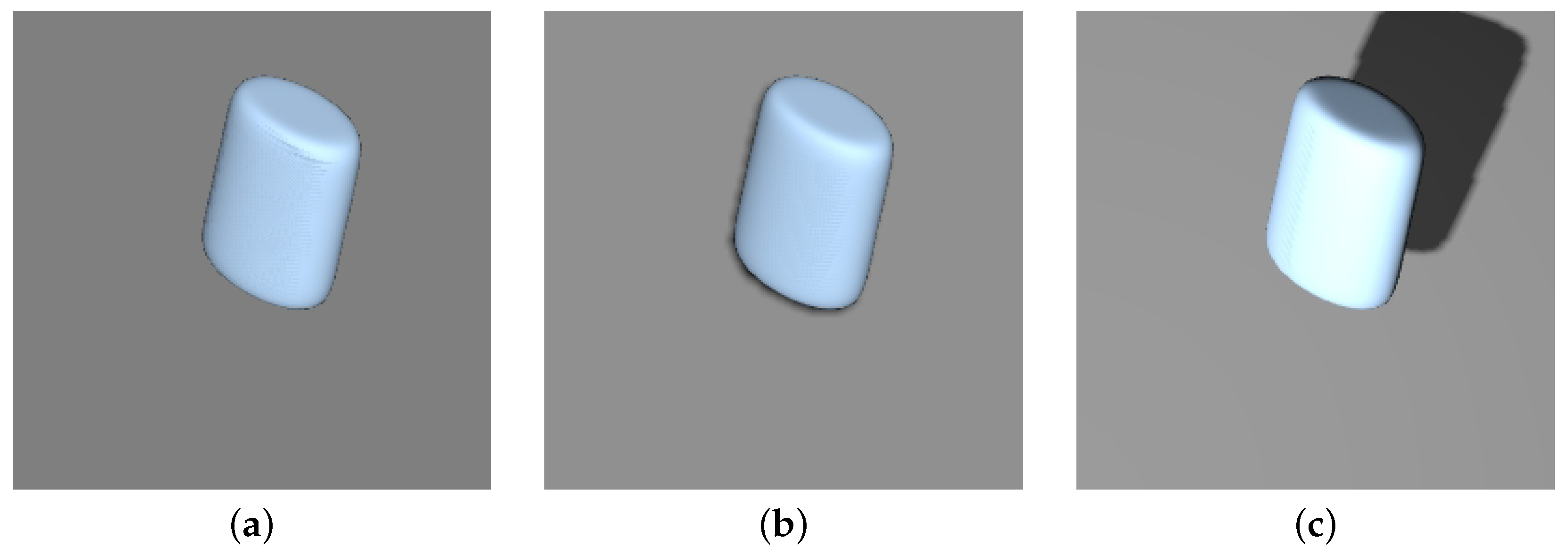
- We propose two data modification methods to combat the lack of spatial information, which helps to reduce the parameter ambiguity and allows for a successful estimation of the superquadric parameters. The first includes fixing the z position parameter of the generated superquadrics, whereas the second relies on the addition of shadow cues to the images.
- We demonstrate that our CNN predictor outperforms current state-of-the-art methods and is also capable of generalizing from synthetic to real images.
2. Related Work
2.1. Superquadric Recovery
2.2. Deep Learning and 3D data
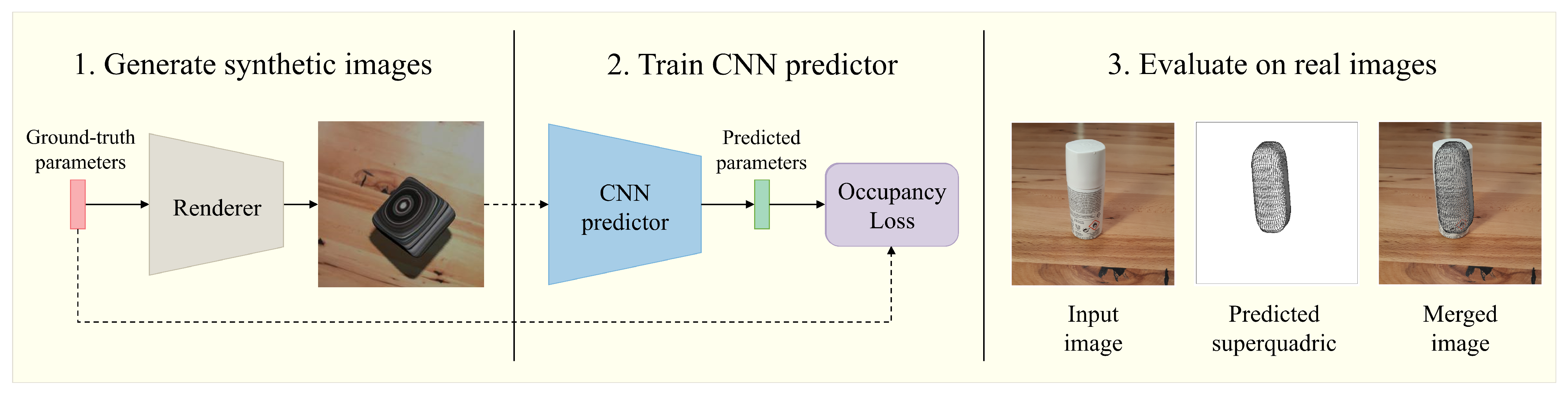
3. Methodology
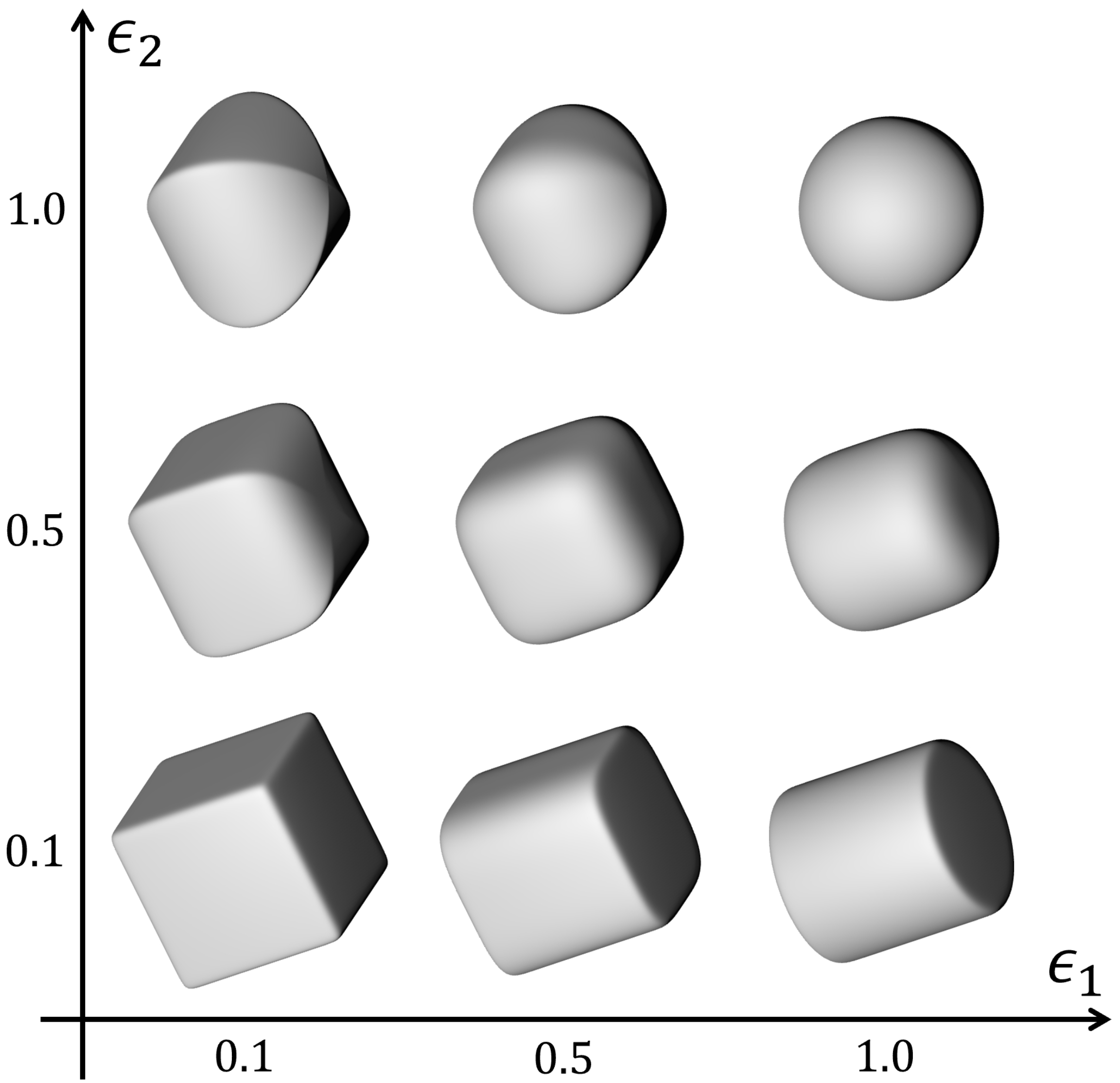
3.1. Superquadrics Definition
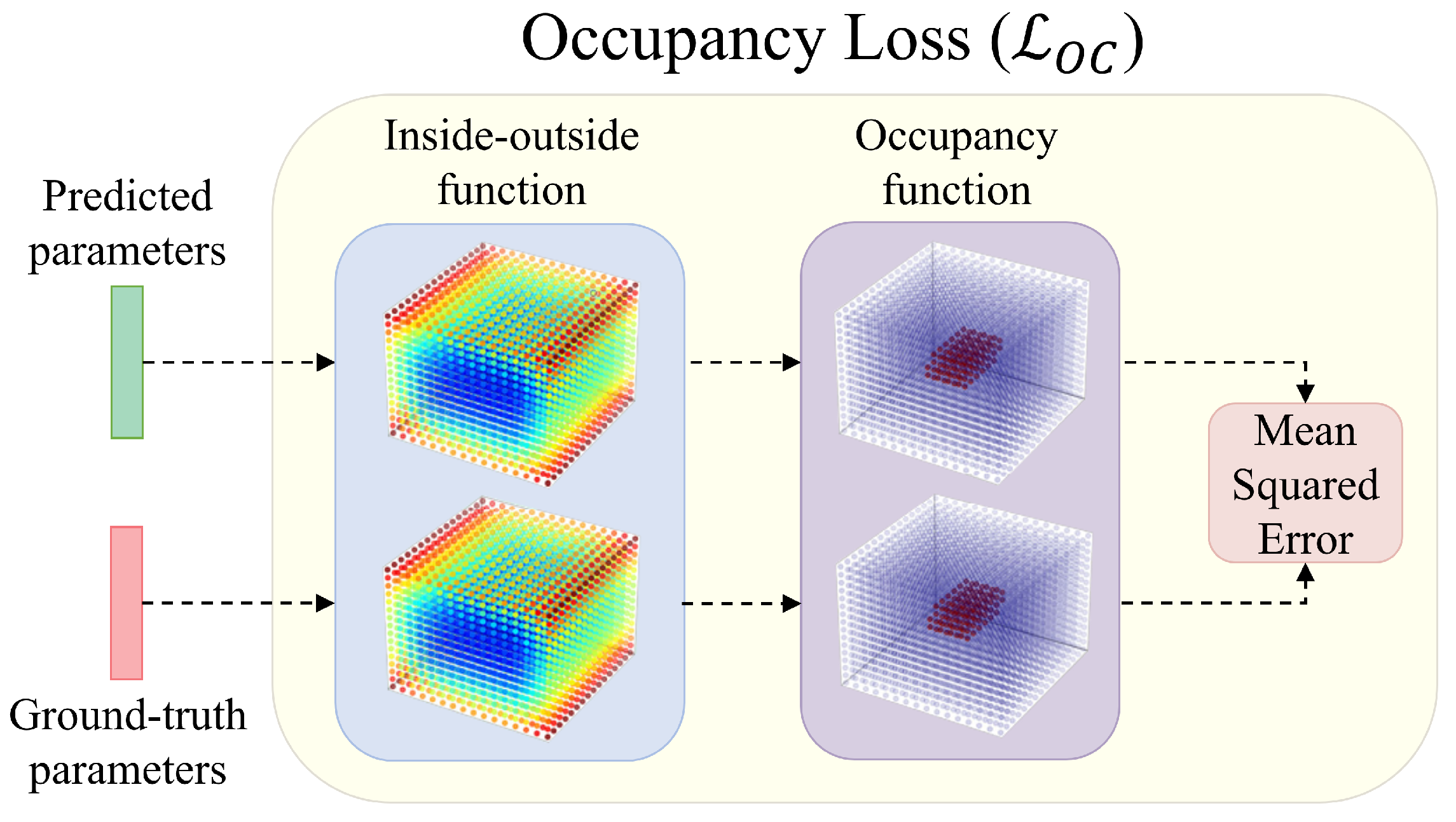
3.2. Problem Definition and Loss Functions
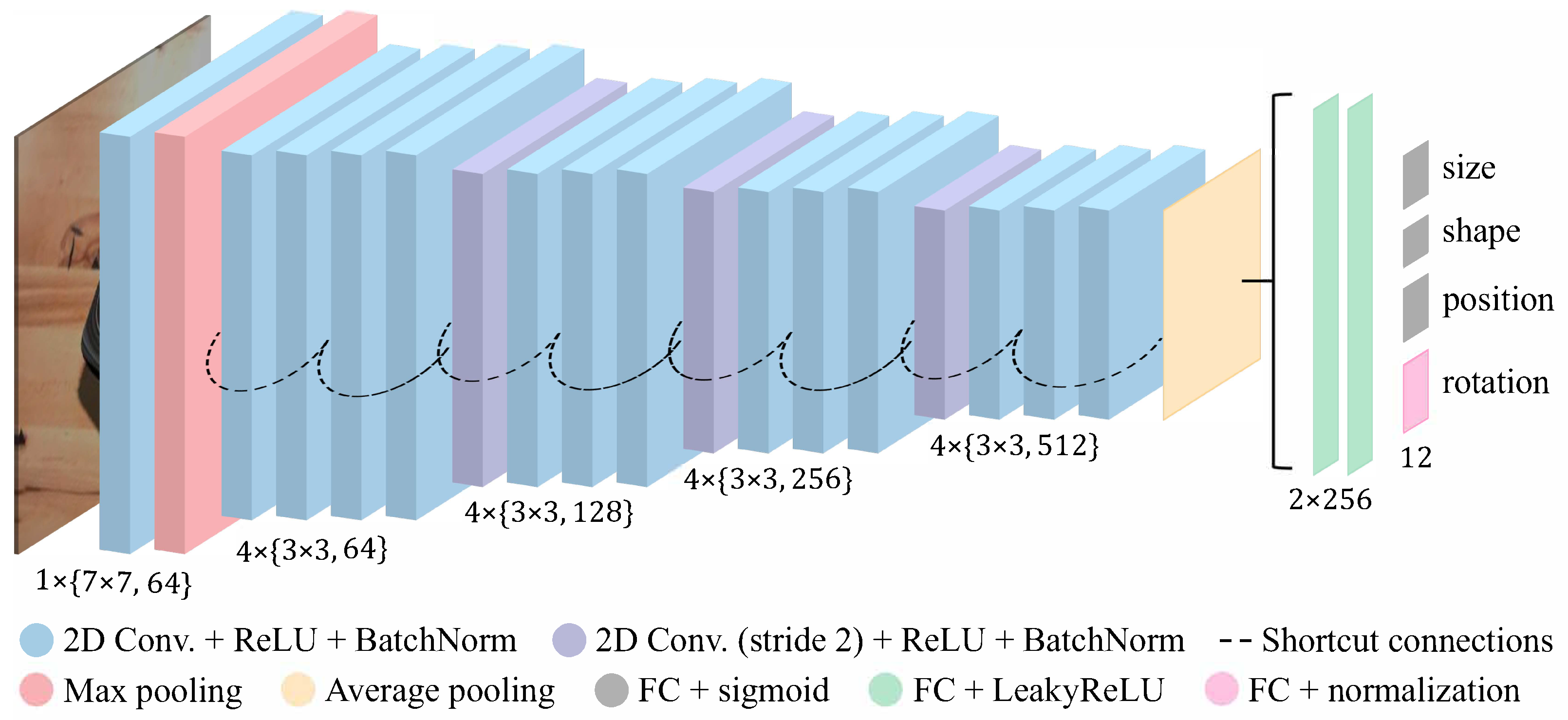
3.3. Neural Network
3.4. Synthetic Data Generation
4. Experiments and Results
4.1. Experiments
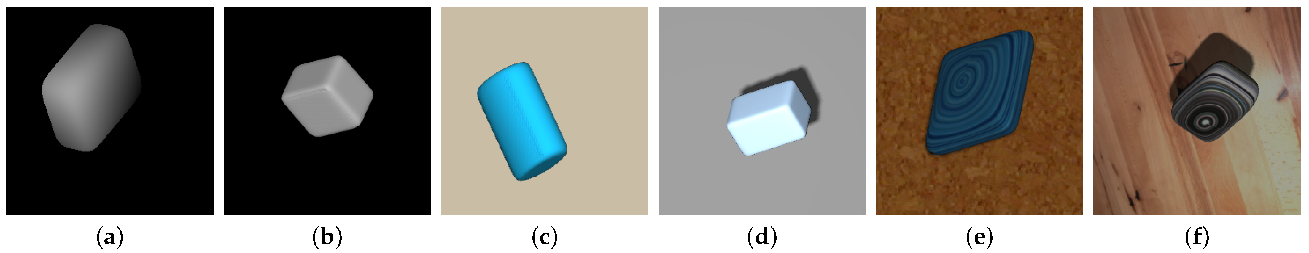
4.2. Datasets
4.3. Performance Metrics
4.4. Training Procedure
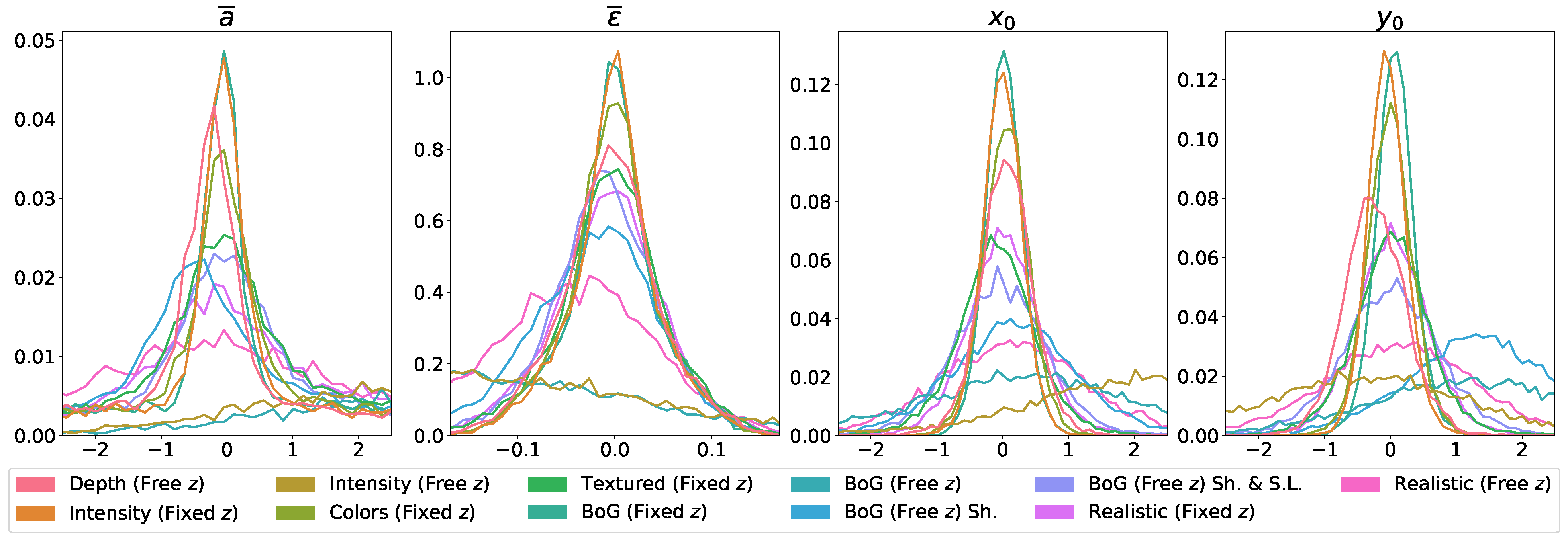
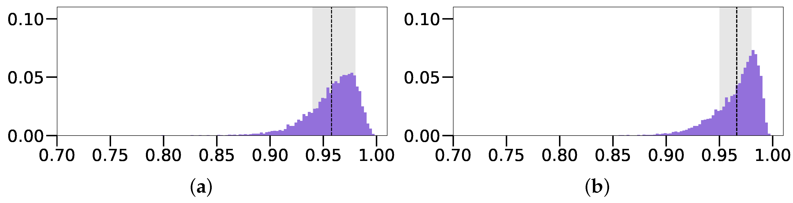
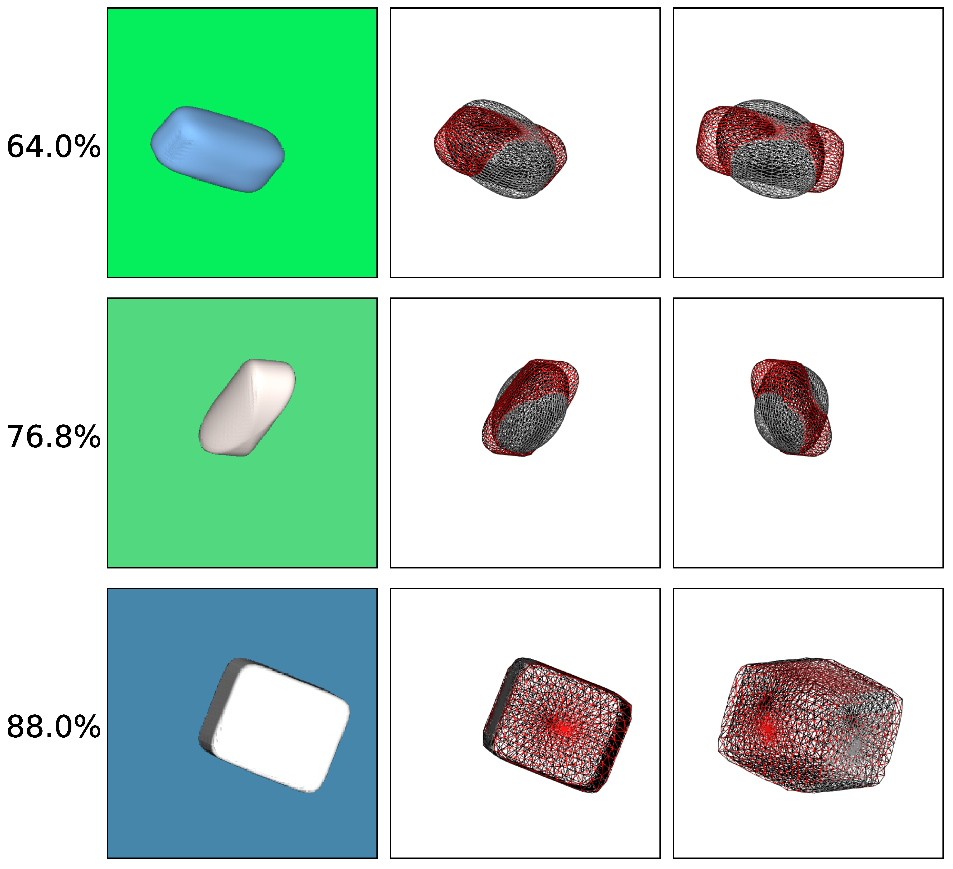
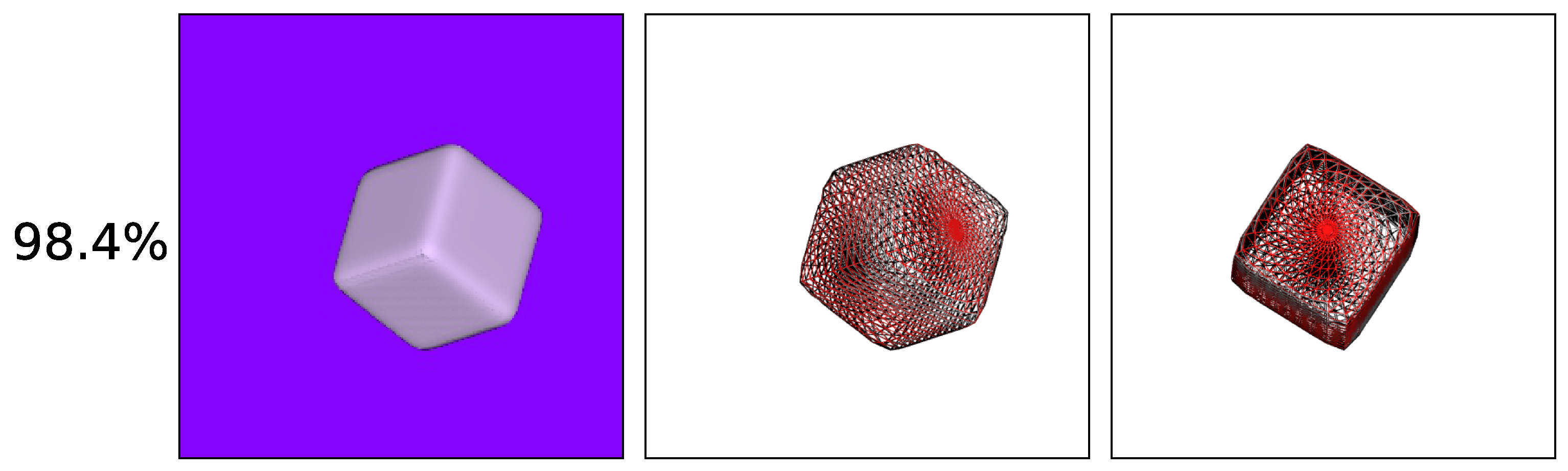
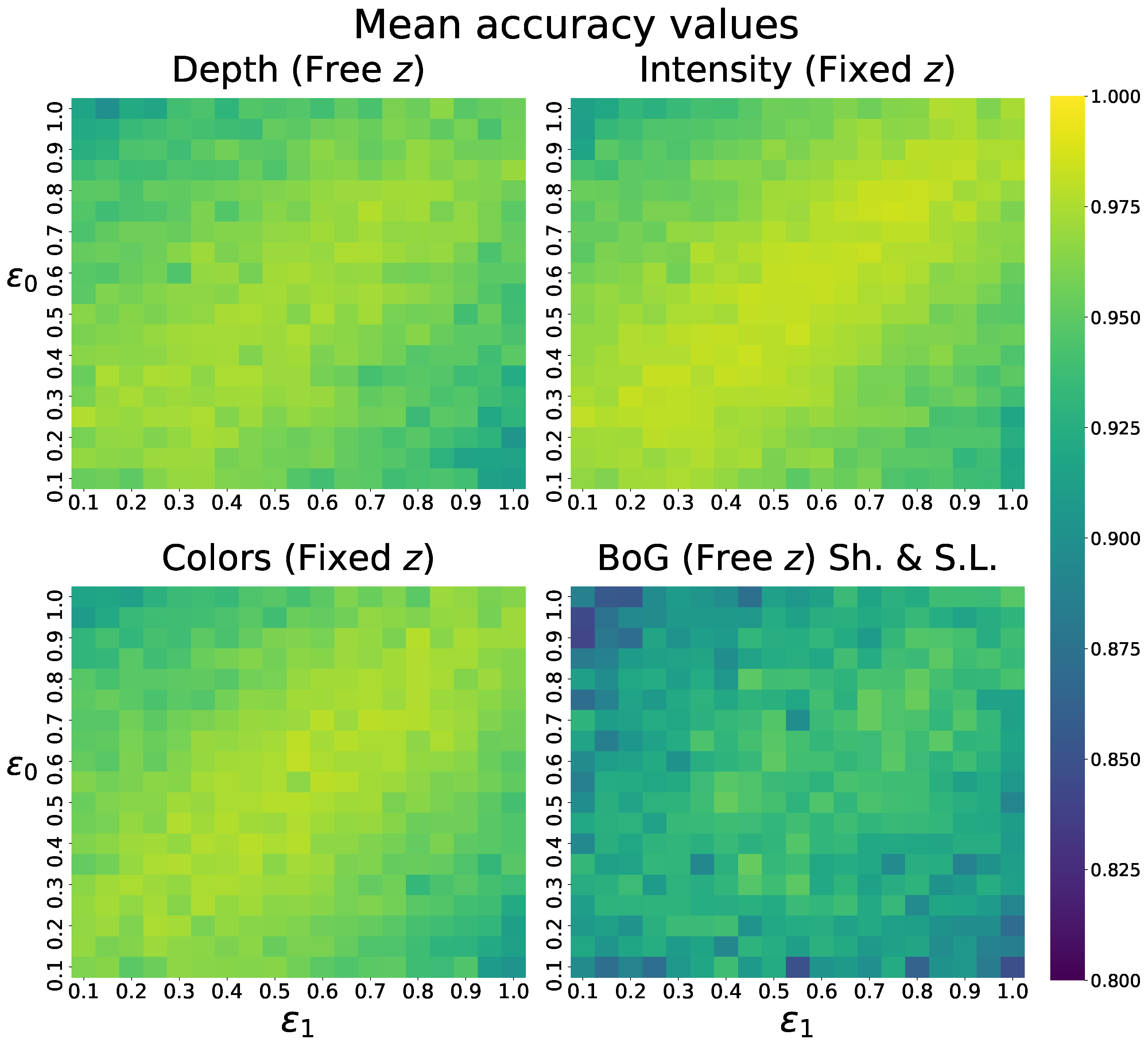
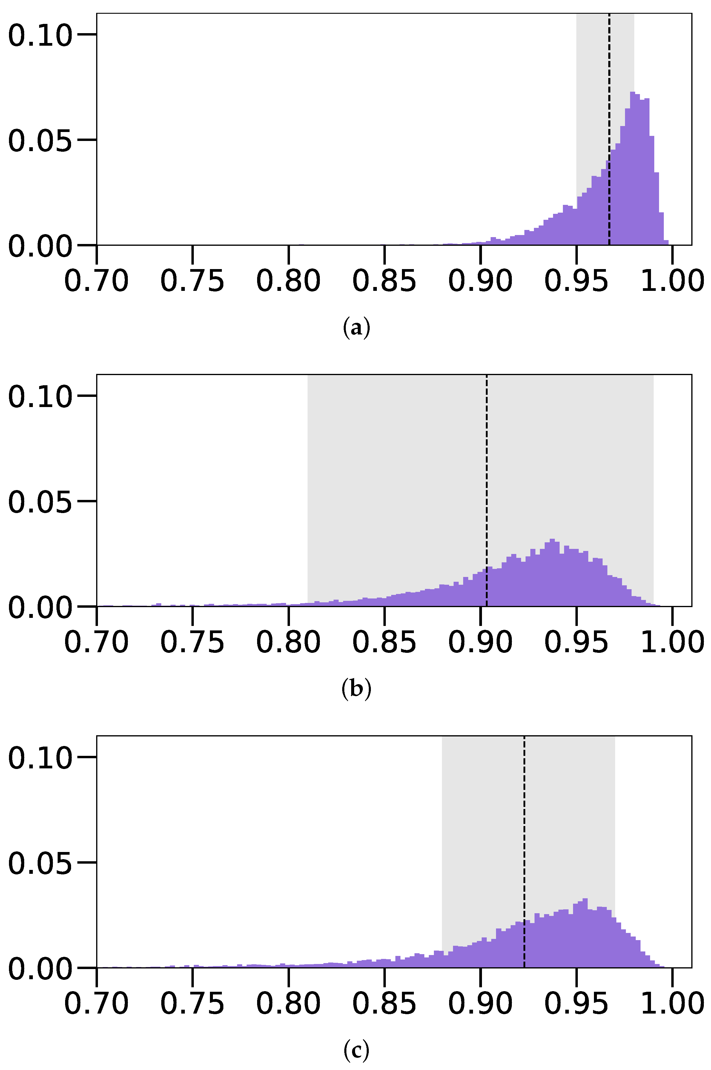
4.5. Results
4.5.1. Reconstruction from 2D Images
4.5.2. Solving the Fixed z Position Requirement
4.5.3. Comparison with the State-of-the-Art
4.5.4. Performance of Different Backbone Architectures
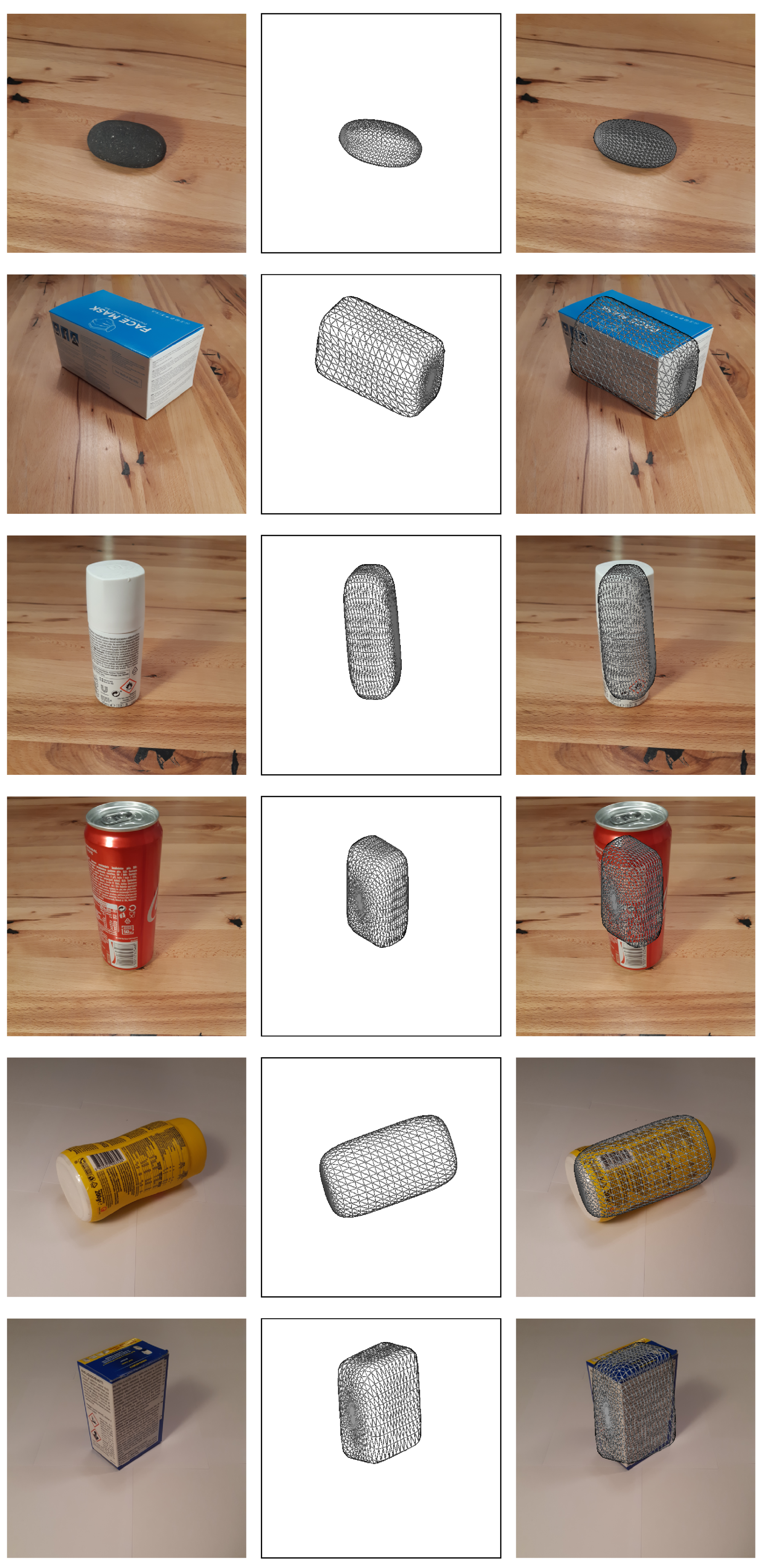
4.5.5. Performance on Real Images
5. Conclusions
Author Contributions
Funding
Institutional Review Board Statement
Informed Consent Statement
Data Availability Statement
Conflicts of Interest
References
- Barr, A.H. Superquadrics and angle-preserving transformations. IEEE Comput. Graph. Appl. 1981, 1, 11–23. [Google Scholar] [CrossRef] [Green Version]
- Solina, F.; Bajcsy, R. Recovery of parametric models from range images: The case for superquadrics with global deformations. IEEE Trans. Pattern Anal. Mach. Intell. 1990, 12, 131–147. [Google Scholar] [CrossRef]
- Khosla, P.; Volpe, R. Superquadric artificial potentials for obstacle avoidance and approach. In Proceedings of the IEEE International Conference on Robotics and Automation, Philadelphia, PA, USA, 24–29 April 1988; pp. 1778–1784. [Google Scholar] [CrossRef]
- Smith, N.E.; Cobb, R.G.; Baker, W.P. Incorporating stochastics into optimal collision avoidance problems using superquadrics. J. Air Transp. 2020, 28, 65–69. [Google Scholar] [CrossRef]
- Mahler, J.; Matl, M.; Satish, V.; Danielczuk, M.; DeRose, B.; McKinley, S.; Goldberg, K. Learning ambidextrous robot grasping policies. Sci. Robot. 2019, 4, eaau4984. [Google Scholar] [CrossRef] [PubMed]
- Morrison, D.; Corke, P.; Leitner, J. Learning robust, real-time, reactive robotic grasping. Int. J. Robot. Res. 2020, 39, 183–201. [Google Scholar] [CrossRef]
- Marr, D. Vision: A Computational Investigation into the Human Representation and Processing of Visual Information; MIT Press: Cambridge, MA, USA, 1982. [Google Scholar] [CrossRef]
- Pentland, A.P. Perceptual organization and the representation of natural form. Artif. Intell. 1986, 28, 293–331. [Google Scholar] [CrossRef]
- Tulsiani, S.; Su, H.; Guibas, L.J.; Efros, A.A.; Malik, J. Learning shape abstractions by assembling volumetric primitives. In Proceedings of the IEEE Conference on Computer Vision and Pattern Recognition, Honolulu, HI, USA, 21–26 July 2017; pp. 2635–2643. [Google Scholar] [CrossRef] [Green Version]
- Paschalidou, D.; Ulusoy, A.O.; Geiger, A. Superquadrics revisited: Learning 3D shape parsing beyond cuboids. In Proceedings of the IEEE/CVF Conference on Computer Vision and Pattern Recognition, Long Beach, CA, USA, 15–20 June 2019; pp. 10344–10353. [Google Scholar] [CrossRef] [Green Version]
- Paschalidou, D.; Gool, L.V.; Geiger, A. Learning unsupervised hierarchical part decomposition of 3D objects from a single RGB image. In Proceedings of the IEEE/CVF Conference on Computer Vision and Pattern Recognition, Seattle, WA, USA, 13–19 June 2020; pp. 1060–1070. [Google Scholar] [CrossRef]
- Oblak, T.; Grm, K.; Jaklič, A.; Peer, P.; Štruc, V.; Solina, F. Recovery of superquadrics from range images using deep learning: A preliminary study. In Proceedings of the IEEE International Work Conference on Bioinspired Intelligence (IWOBI), Budapest, Hungary, 3–5 July 2019; pp. 45–52. [Google Scholar] [CrossRef]
- Oblak, T.; Šircelj, J.; Štruc, V.; Peer, P.; Solina, F.; Jaklič, A. Learning to Predict Superquadric Parameters From Depth Images With Explicit and Implicit Supervision. IEEE Access 2020, 9, 1087–1102. [Google Scholar] [CrossRef]
- Šircelj, J.; Oblak, T.; Grm, K.; Petković, U.; Jaklič, A.; Peer, P.; Štruc, V.; Solina, F. Segmentation and recovery of superquadric models using convolutional neural networks. In Proceedings of the 25th Computer Vision Winter Workshop, Rogaška Slatina, Slovenia, 3–5 February 2020; pp. 1–5. [Google Scholar]
- Li, S.; Liu, M.; Walder, C. EditVAE: Unsupervised Part-Aware Controllable 3D Point Cloud Shape Generation. arXiv 2021, arXiv:2110.06679. [Google Scholar] [CrossRef]
- Abrams, A.; Miskell, K.; Pless, R. The episolar constraint: Monocular shape from shadow correspondence. In Proceedings of the IEEE Conference on Computer Vision and Pattern Recognition, Portland, OR, USA, 23–28 June 2013; pp. 1407–1414. [Google Scholar] [CrossRef]
- Xie, Y.; Feng, D.; Xiong, S.; Zhu, J.; Liu, Y. Multi-Scene Building Height Estimation Method Based on Shadow in High Resolution Imagery. Remote Sens. 2021, 13, 2862. [Google Scholar] [CrossRef]
- Vezzani, G.; Pattacini, U.; Natale, L. A grasping approach based on superquadric models. In Proceedings of the IEEE International Conference on Robotics and Automation (ICRA), Singapore, 29 May–3 June 2017; pp. 1579–1586. [Google Scholar] [CrossRef]
- Makhal, A.; Thomas, F.; Gracia, A.P. Grasping unknown objects in clutter by superquadric representation. In Proceedings of the 2nd IEEE International Conference on Robotic Computing (IRC), Laguna Hills, CA, USA, 31 January–2 February 2018; pp. 292–299. [Google Scholar] [CrossRef] [Green Version]
- Vezzani, G.; Pattacini, U.; Pasquale, G.; Natale, L. Improving Superquadric Modeling and Grasping with Prior on Object Shapes. In Proceedings of the IEEE International Conference on Robotics and Automation (ICRA), Brisbane, Australia, 21–25 May 2018; pp. 6875–6882. [Google Scholar] [CrossRef]
- Haschke, R.; Walck, G.; Ritter, H. Geometry-Based Grasping Pipeline for Bi-Modal Pick and Place. In Proceedings of the IEEE/RSJ International Conference on Intelligent Robots and Systems (IROS), Prague, Czech Republic, 27 September–1 October 2021; pp. 4002–4008. [Google Scholar] [CrossRef]
- Solina, F.; Bajcsy, R. Range image interpretation of mail pieces with superquadrics. In Proceedings of the National Conference on Artificial Intelligence, Seattle, WA, USA, 13–17 July 1987; Volume 2, pp. 733–737. [Google Scholar]
- Jaklič, A.; Erič, M.; Mihajlović, I.; Stopinšek, Ž.; Solina, F. Volumetric models from 3D point clouds: The case study of sarcophagi cargo from a 2nd/3rd century AD Roman shipwreck near Sutivan on island Brač, Croatia. J. Archaeol. Sci. 2015, 62, 143–152. [Google Scholar] [CrossRef]
- Stopinšek, Ž.; Solina, F. 3D modeliranje podvodnih posnetkov. In SI Robotika; Munih, M., Ed.; Slovenska Matica: Ljubljana, Slovenia, 2017; pp. 103–114. [Google Scholar]
- Hachiuma, R.; Saito, H. Volumetric Representation of Semantically Segmented Human Body Parts Using Superquadrics. In Proceedings of the International Conference on Virtual Reality and Augmented Reality, Tallinn, Estonia, 23–25 October 2019; Springer: Berlin/Heidelberg, Germany, 2019; pp. 52–61. [Google Scholar] [CrossRef]
- Pentland, A.P. Recognition by parts. In Proceedings of the IEEE 1st International Conference on Computer Vision, London, UK, 8–11 June 1987; pp. 612–620. [Google Scholar] [CrossRef]
- Boult, T.E.; Gross, A.D. Recovery of superquadrics from 3D information. In Proceedings of the Intelligent Robots and Computer Vision VI, Cambridge, MA, USA, 2–6 November 1988; International Society for Optics and Photonics: Washington, DC, USA, 1988; Volume 848, pp. 358–365. [Google Scholar] [CrossRef]
- Gross, A.D.; Boult, T.E. Error of fit measures for recovering parametric solids. In Proceedings of the 2nd International Conference of Computer Vision, Tampa, FL, USA, 5–8 December 1988; pp. 690–694. [Google Scholar] [CrossRef]
- Ferrie, F.P.; Lagarde, J.; Whaite, P. Darboux frames, snakes, and super-quadrics: Geometry from the bottom up. IEEE Trans. Pattern Anal. Mach. Intell. 1993, 15, 771–784. [Google Scholar] [CrossRef]
- Hanson, A.J. Hyperquadrics: Smoothly deformable shapes with convex polyhedral bounds. Comput. Vision Graph. Image Process. 1988, 44, 191–210. [Google Scholar] [CrossRef]
- Terzopoulos, D.; Metaxas, D. Dynamic 3D models with local and global deformations: Deformable superquadrics. IEEE Trans. Pattern Anal. Mach. Intell. 1991, 13, 703–714. [Google Scholar] [CrossRef] [Green Version]
- Leonardis, A.; Jaklič, A.; Solina, F. Superquadrics for segmenting and modeling range data. IEEE Trans. Pattern Anal. Mach. Intell. 1997, 19, 1289–1295. [Google Scholar] [CrossRef] [Green Version]
- Krivic, J.; Solina, F. Part-level object recognition using superquadrics. Comput. Vis. Image Underst. 2004, 95, 105–126. [Google Scholar] [CrossRef] [Green Version]
- Slabanja, J.; Meden, B.; Peer, P.; Jaklič, A.; Solina, F. Segmentation and reconstruction of 3D models from a point cloud with deep neural networks. In Proceedings of the International Conference on Information and Communication Technology Convergence (ICTC), Jeju Island, Korea, 17–19 October 2018; pp. 118–123. [Google Scholar] [CrossRef]
- Wu, Z.; Song, S.; Khosla, A.; Yu, F.; Zhang, L.; Tang, X.; Xiao, J. 3D shapenets: A deep representation for volumetric shapes. In Proceedings of the IEEE Conference on Computer Vision and Pattern Recognition, Boston, MA, USA, 7–12 June 2015; pp. 1912–1920. [Google Scholar] [CrossRef] [Green Version]
- Wu, J.; Wang, Y.; Xue, T.; Sun, X.; Freeman, B.; Tenenbaum, J. MarrNet: 3D Shape Reconstruction via 2.5D Sketches. Adv. Neural Inf. Process. Syst. 2017, 30, 540–550. [Google Scholar]
- Miao, S.; Wang, Z.J.; Liao, R. A CNN regression approach for real-time 2D/3D registration. IEEE Trans. Med. Imaging 2016, 35, 1352–1363. [Google Scholar] [CrossRef] [PubMed]
- Zhu, R.; Kiani Galoogahi, H.; Wang, C.; Lucey, S. Rethinking reprojection: Closing the loop for pose-aware shape reconstruction from a single image. In Proceedings of the IEEE International Conference on Computer Vision, Venice, Italy, 22–29 October 2017; pp. 57–65. [Google Scholar] [CrossRef] [Green Version]
- Xiang, Y.; Schmidt, T.; Narayanan, V.; Fox, D. PoseCNN: A Convolutional Neural Network for 6D Object Pose Estimation in Cluttered Scenes. In Proceedings of the 14th Robotics: Science and Systems (RSS), Pittsburgh, PA, USA, 26–30 June 2018; pp. 1–10. [Google Scholar] [CrossRef]
- Kuipers, J.B. Quaternions and Rotation Sequences: A Primer with Applications to Orbits, Aerospace, and Virtual Reality; Princeton University Press: Princeton, NJ, USA, 1999. [Google Scholar] [CrossRef]
- Jaklič, A.; Leonardis, A.; Solina, F. Segmentation and Recovery of Superquadrics; Springer Science & Business Media: New York, NY, USA, 2000; Volume 20. [Google Scholar] [CrossRef]
- He, K.; Zhang, X.; Ren, S.; Sun, J. Deep residual learning for image recognition. In Proceedings of the IEEE Conference on Computer Vision and Pattern Recognition, Las Vegas, NV, USA, 27–30 June 2016; pp. 770–778. [Google Scholar]
- Shoemake, K. Uniform random rotations. In Graphics Gems III (IBM Version); Elsevier: Amsterdam, The Netherland, 1992; pp. 124–132. [Google Scholar] [CrossRef]
- Oechsle, M.; Mescheder, L.; Niemeyer, M.; Strauss, T.; Geiger, A. Texture fields: Learning texture representations in function space. In Proceedings of the IEEE/CVF International Conference on Computer Vision, Seoul, Korea, 27 October–2 November 2019; pp. 4531–4540. [Google Scholar] [CrossRef] [Green Version]
- Deng, J.; Dong, W.; Socher, R.; Li, L.J.; Li, K.; Fei-Fei, L. ImageNet: A large-scale hierarchical image database. In Proceedings of the IEEE Conference on Computer Vision and Pattern Recognition, Miami, FL, USA, 20–25 June 2009; pp. 248–255. [Google Scholar] [CrossRef] [Green Version]
- Kingma, D.P.; Ba, J.L. Adam: A method for stochastic optimization. In Proceedings of the International Conference on Learning Representations, San Diego, CA, USA, 7–9 May 2015; pp. 1–5. [Google Scholar]
- Bengio, Y. Practical recommendations for gradient-based training of deep architectures. In Neural Networks: Tricks of the Trade; Springer: Berlin/Heidelberg, Germany, 2012; pp. 437–478. [Google Scholar] [CrossRef] [Green Version]
- Keskar, N.S.; Nocedal, J.; Tang, P.T.P.; Mudigere, D.; Smelyanskiy, M. On large-batch training for deep learning: Generalization gap and sharp minima. In Proceedings of the 5th International Conference on Learning Representations, Toulon, France, 24–26 April 2017; pp. 1–8. [Google Scholar]
- Kandel, I.; Castelli, M. The effect of batch size on the generalizability of the convolutional neural networks on a histopathology dataset. ICT Express 2020, 6, 312–315. [Google Scholar] [CrossRef]
- Szegedy, C.; Vanhoucke, V.; Ioffe, S.; Shlens, J.; Wojna, Z. Rethinking the inception architecture for computer vision. In Proceedings of the IEEE Conference on Computer Vision and Pattern Recognition, Las Vegas, NV, USA, 27–30 June 2016; pp. 2818–2826. [Google Scholar]


| Experiment Dataset | Size [0–255] | Shape [0–1] | Position [0–255] | IoU [%] | ||
|---|---|---|---|---|---|---|
| Depth (Oblak et al. [13]) | ||||||
| Intensity (Fixed z) | / | |||||
| Intensity (Free z) | ||||||
| Colors (Fixed z) | / | |||||
| Textured (Fixed z) | / | |||||
| Blue on Gray (Fixed z) | / | |||||
| Blue on Gray (Free z) | ||||||
| Blue on Gray (Free z) with Sh. | ||||||
| Blue on Gray (Free z) with Sh. & S.L. | ||||||
| Textured on Wood (Fixed z) with Sh. & S.L. | / | |||||
| Textured on Wood (Free z) with Sh. & S.L. | ||||||
| Experiment Dataset | Method | IoU |
|---|---|---|
| Intensity (Fixed z) | Ours | 0.966 ± 0.022 |
| Paschalidou et al. [10] | ||
| Sub. Intensity (Fixed z) | Ours | 0.972 ± 0.018 |
| Paschalidou et al. [10] | ||
| BoG (Free z) with Sh. & S.L. | Ours | 0.923 ± 0.052 |
| Paschalidou et al. [10] | ||
| Sub. BoG (Free z) with Sh. & S.L. | Ours | 0.932 ± 0.044 |
| Paschalidou et al. [10] |
| Experiment Dataset | Architecture | IoU |
|---|---|---|
| Intensity (Fixed z) | ResNet-18 | 0.966 ± 0.022 |
| Inception-V3 | ||
| BoG (Free z) with Sh. & S.L. | ResNet-18 | 0.923 ± 0.052 |
| Inception-V3 | 0.913 ± 0.108 |
Publisher’s Note: MDPI stays neutral with regard to jurisdictional claims in published maps and institutional affiliations. |
© 2022 by the authors. Licensee MDPI, Basel, Switzerland. This article is an open access article distributed under the terms and conditions of the Creative Commons Attribution (CC BY) license (https://creativecommons.org/licenses/by/4.0/).
Share and Cite
Tomašević, D.; Peer, P.; Solina, F.; Jaklič, A.; Štruc, V. Reconstructing Superquadrics from Intensity and Color Images. Sensors 2022, 22, 5332. https://doi.org/10.3390/s22145332
Tomašević D, Peer P, Solina F, Jaklič A, Štruc V. Reconstructing Superquadrics from Intensity and Color Images. Sensors. 2022; 22(14):5332. https://doi.org/10.3390/s22145332
Chicago/Turabian StyleTomašević, Darian, Peter Peer, Franc Solina, Aleš Jaklič, and Vitomir Štruc. 2022. "Reconstructing Superquadrics from Intensity and Color Images" Sensors 22, no. 14: 5332. https://doi.org/10.3390/s22145332