Author Contributions
Conceptualization, J.G.-G., L.G.G.-V., T.S.-J. and A.G.-E.; methodology, J.G.-G. and L.G.G.-V.; investigation, J.G.-G.; software, J.G.-G.; writing—original draft preparation, J.G.-G.; visualization, J.G.-G.; writing—review and editing, J.G.-G., L.G.G.-V., T.S.-J., A.G.-E., E.C.-U. and J.A.E.C.; supervision, L.G.G.-V., T.S.-J. and A.G.-E.; All authors have read and agreed to the published version of the manuscript.
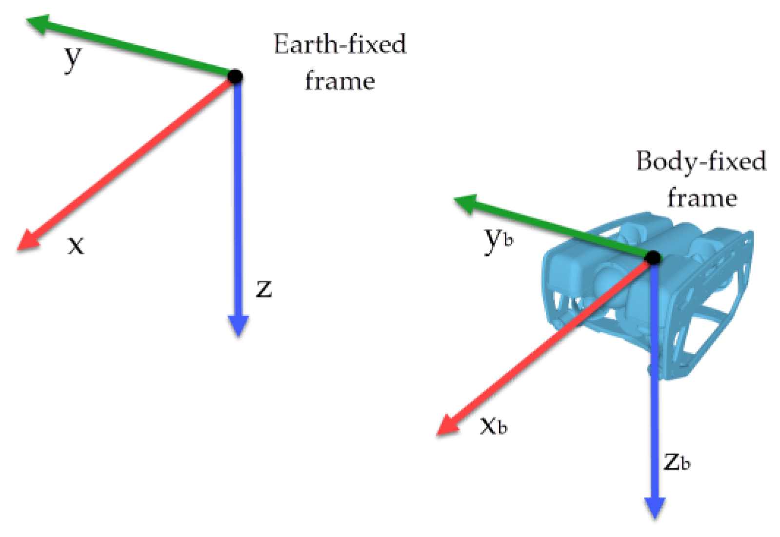
Figure 1.
Reference frames for underwater vehicles.
Figure 1.
Reference frames for underwater vehicles.
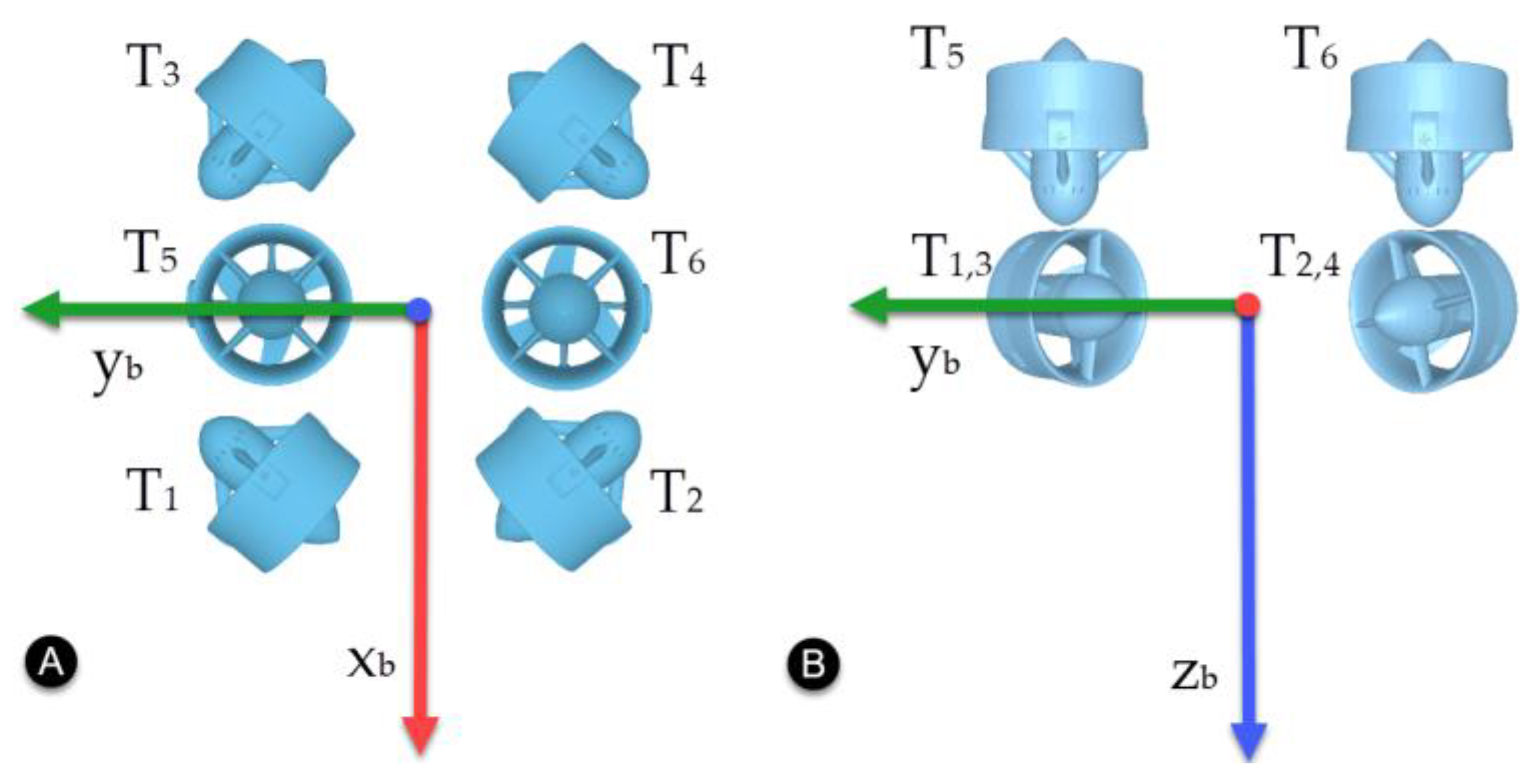
Figure 2.
Thruster configuration for the BlueROV2. (A) Top view. (B) Front view.
Figure 2.
Thruster configuration for the BlueROV2. (A) Top view. (B) Front view.
Figure 3.
BlueROV2 simulator. Simulink block diagram.
Figure 3.
BlueROV2 simulator. Simulink block diagram.
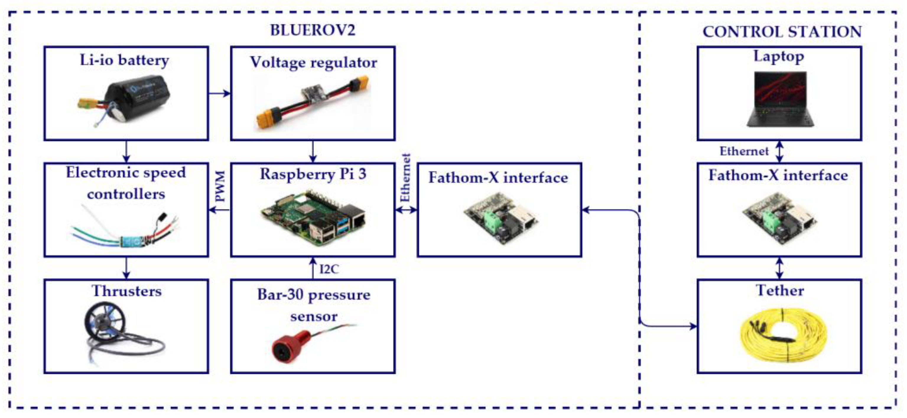
Figure 4.
Experimental set-up, hardware configuration.
Figure 4.
Experimental set-up, hardware configuration.
Figure 5.
Additional thruster for external disturbance. (A) Front view diagram. (B) Implementation.
Figure 5.
Additional thruster for external disturbance. (A) Front view diagram. (B) Implementation.
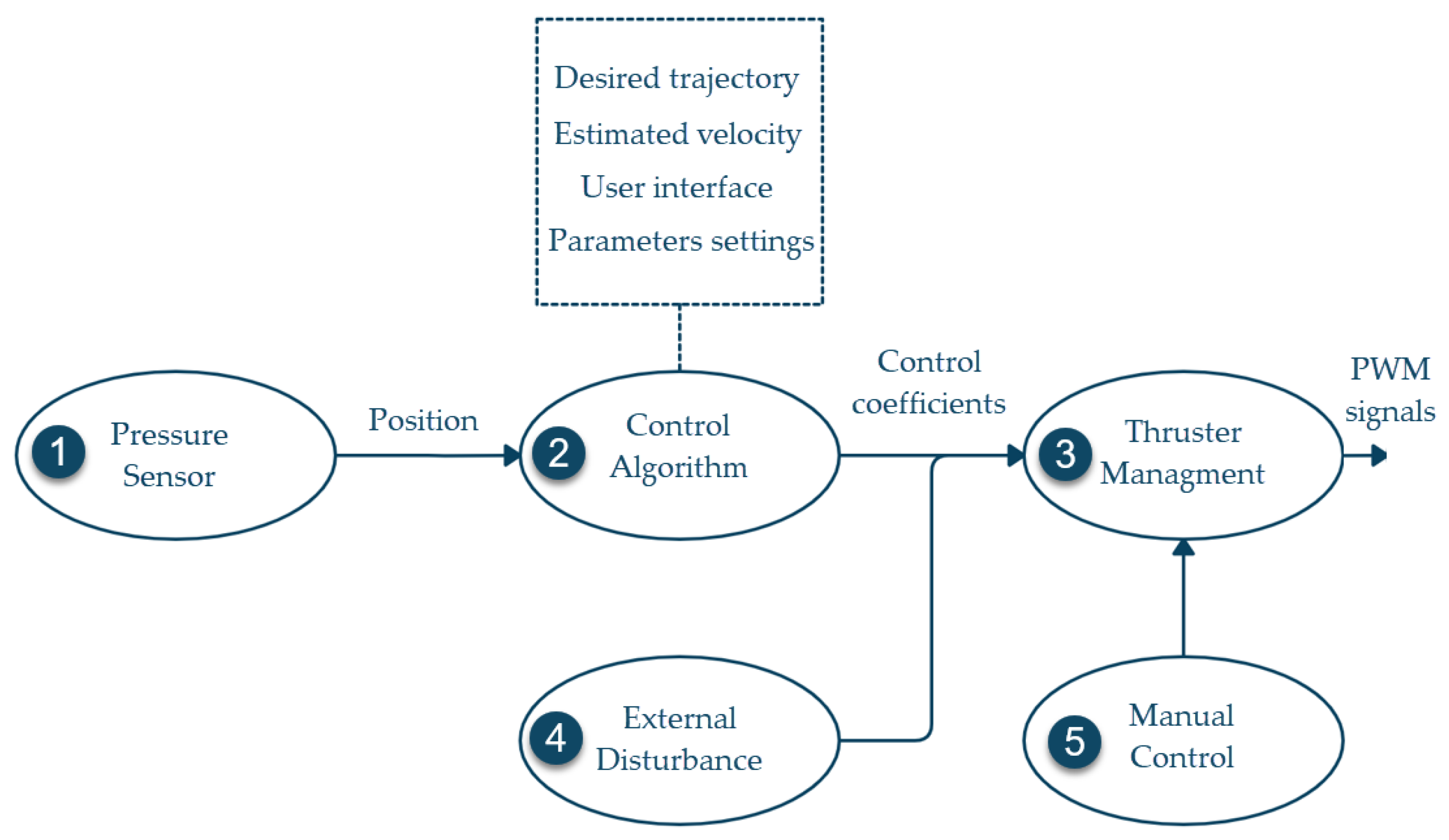
Figure 6.
BlueROV2 software configuration.
Figure 6.
BlueROV2 software configuration.
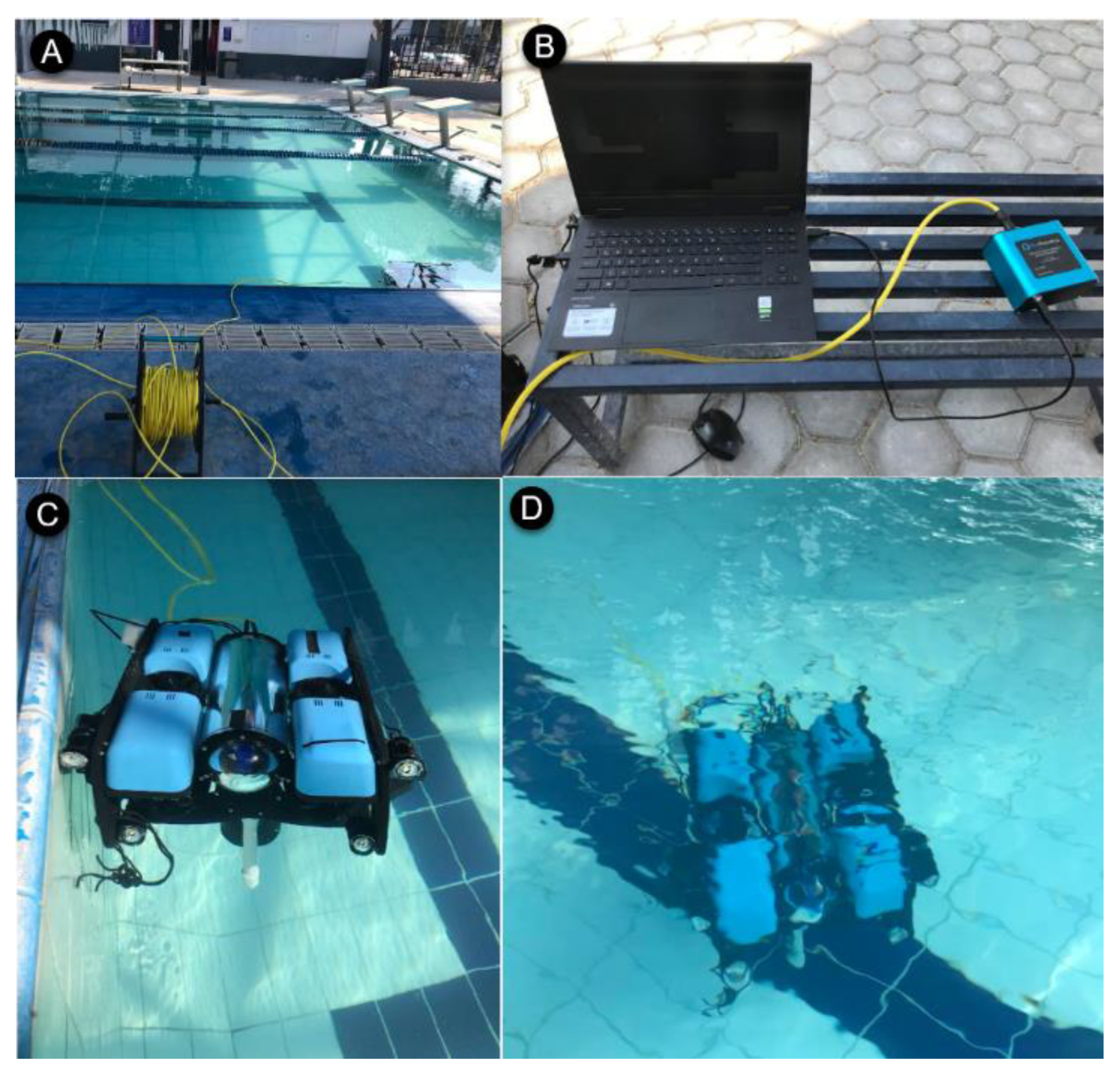
Figure 7.
Experimental set-up. (A) Semi-Olympic swimming pool. (B) Control station. (C) BlueROV2 deployment. (D) Station-keeping task execution.
Figure 7.
Experimental set-up. (A) Semi-Olympic swimming pool. (B) Control station. (C) BlueROV2 deployment. (D) Station-keeping task execution.
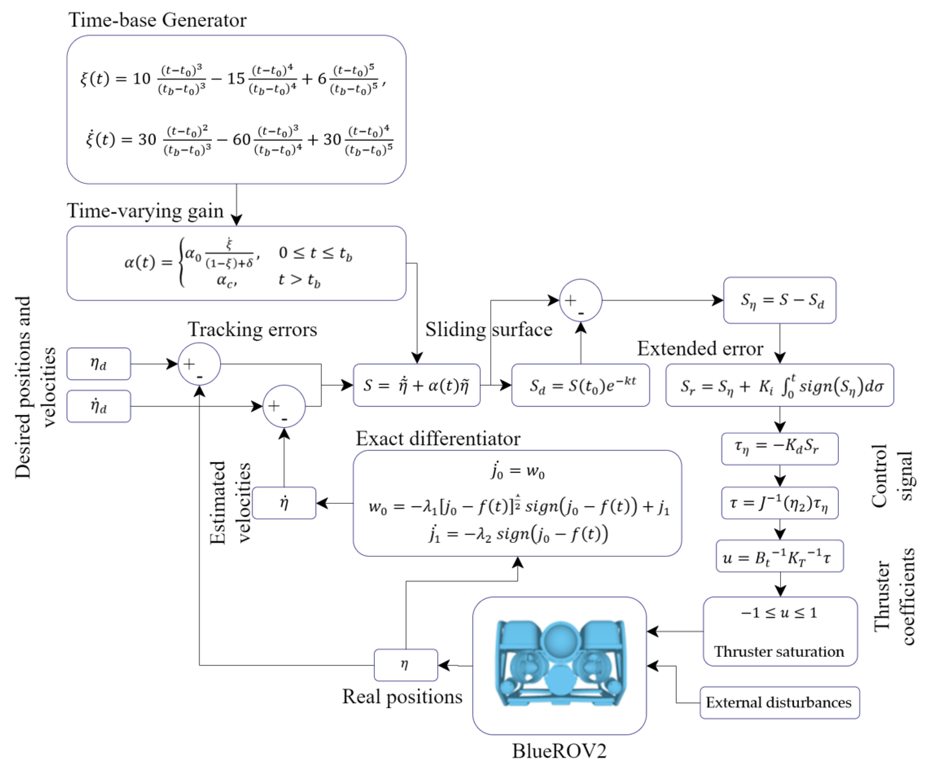
Figure 8.
Block diagram of the proposed controller.
Figure 8.
Block diagram of the proposed controller.
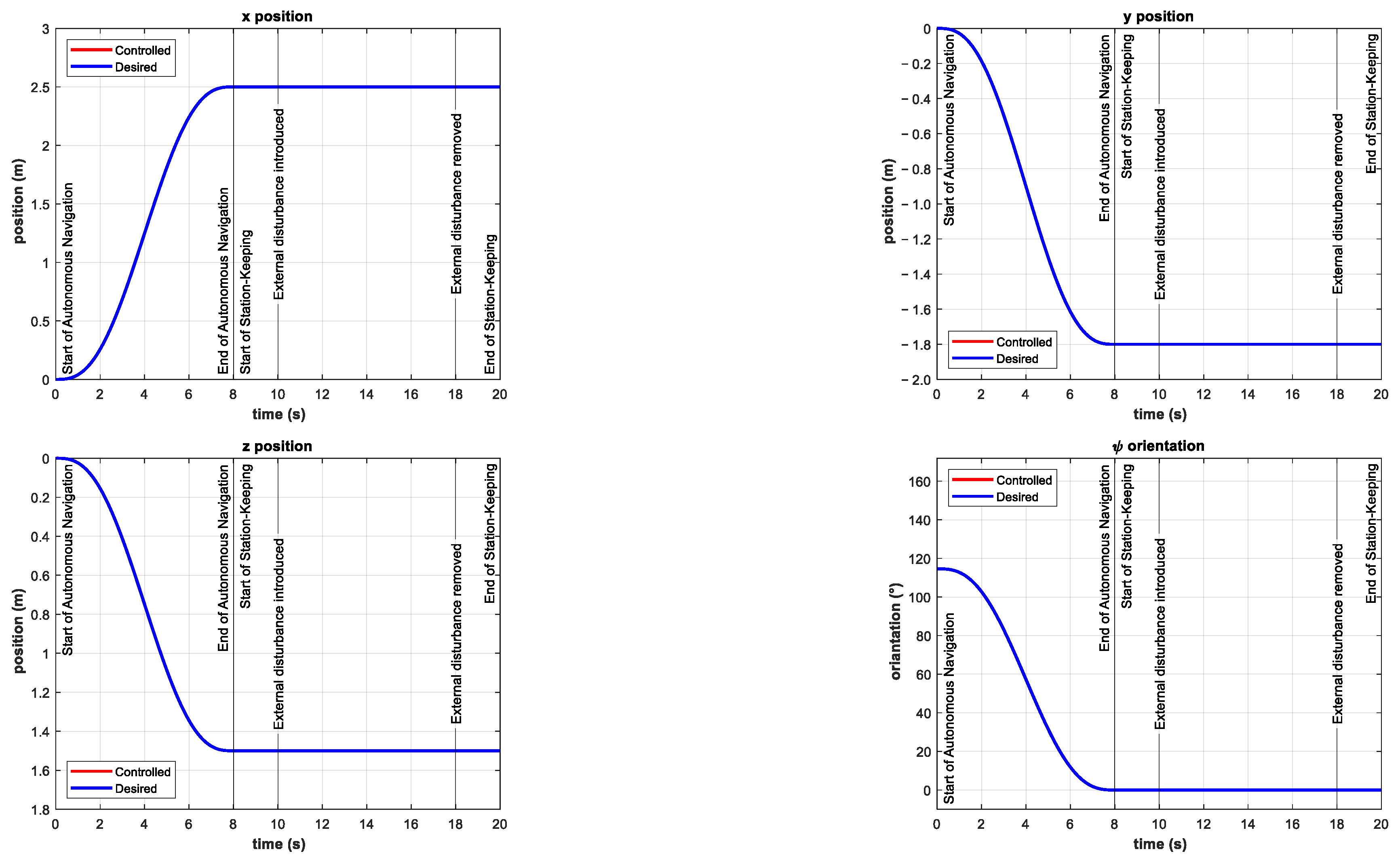
Figure 9.
Simulation results for finite-time trajectory tracking and station-keeping in the , , positions and orientation. External disturbances were introduced in the interval as ocean currents .
Figure 9.
Simulation results for finite-time trajectory tracking and station-keeping in the , , positions and orientation. External disturbances were introduced in the interval as ocean currents .
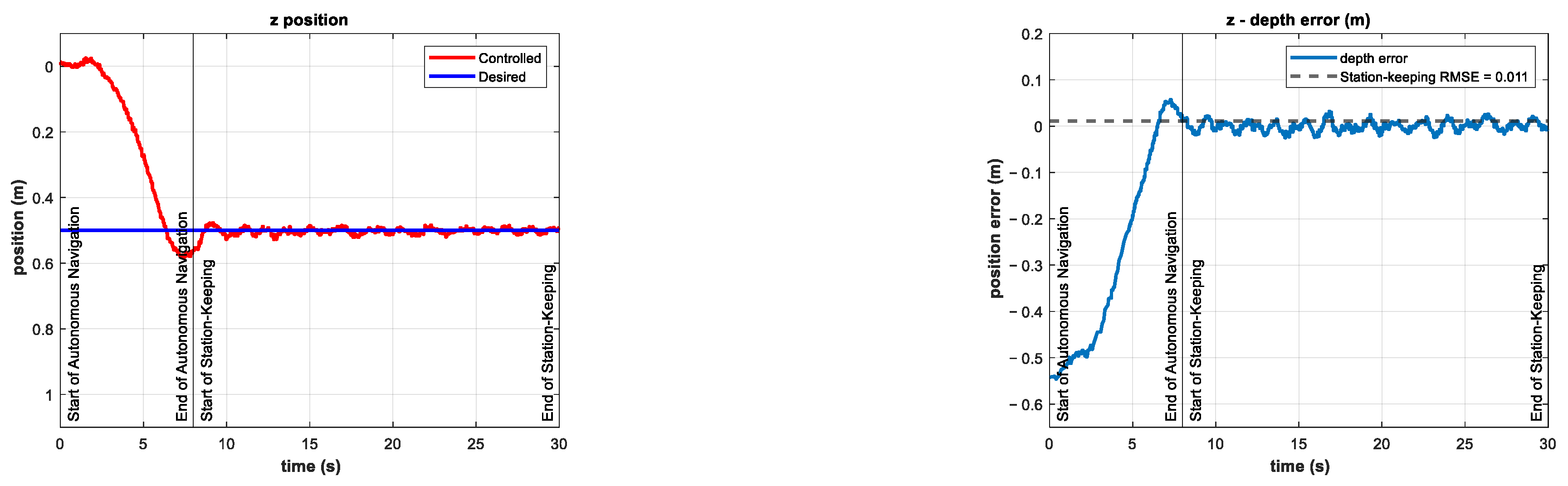
Figure 10.
Depth (left) and tracking error (right) results of the control test. No external disturbances were introduced.
Figure 10.
Depth (left) and tracking error (right) results of the control test. No external disturbances were introduced.
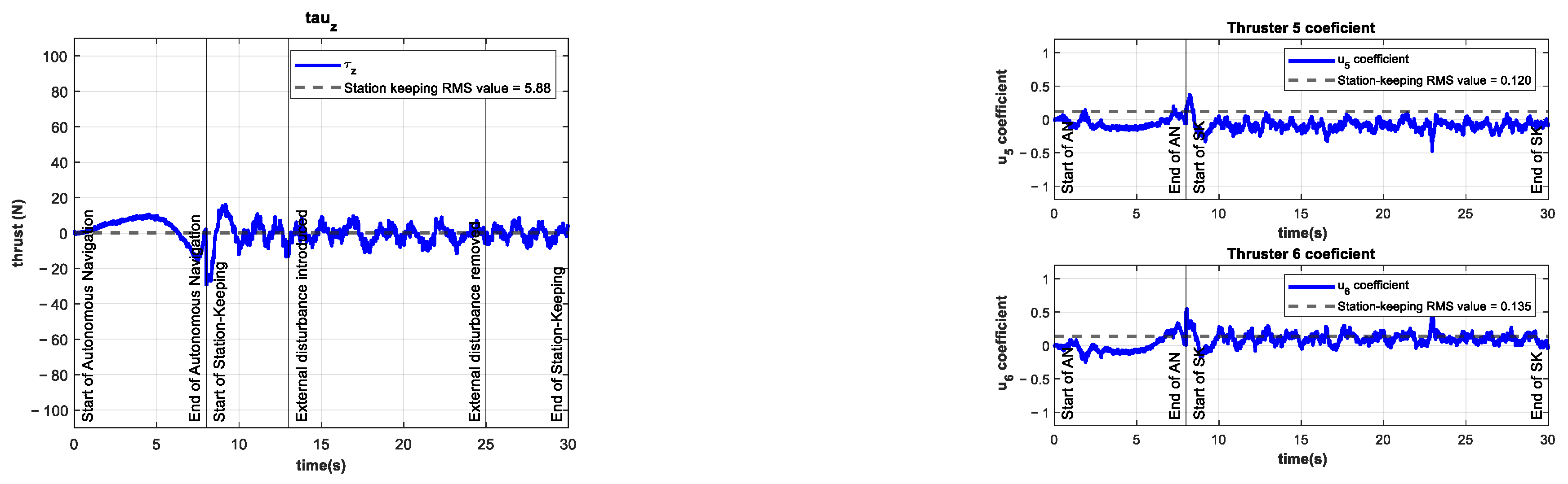
Figure 11.
Experimental results of the control test for depth station-keeping. Control signal (left) and thruster coefficients , (right). No external disturbances were introduced.
Figure 11.
Experimental results of the control test for depth station-keeping. Control signal (left) and thruster coefficients , (right). No external disturbances were introduced.
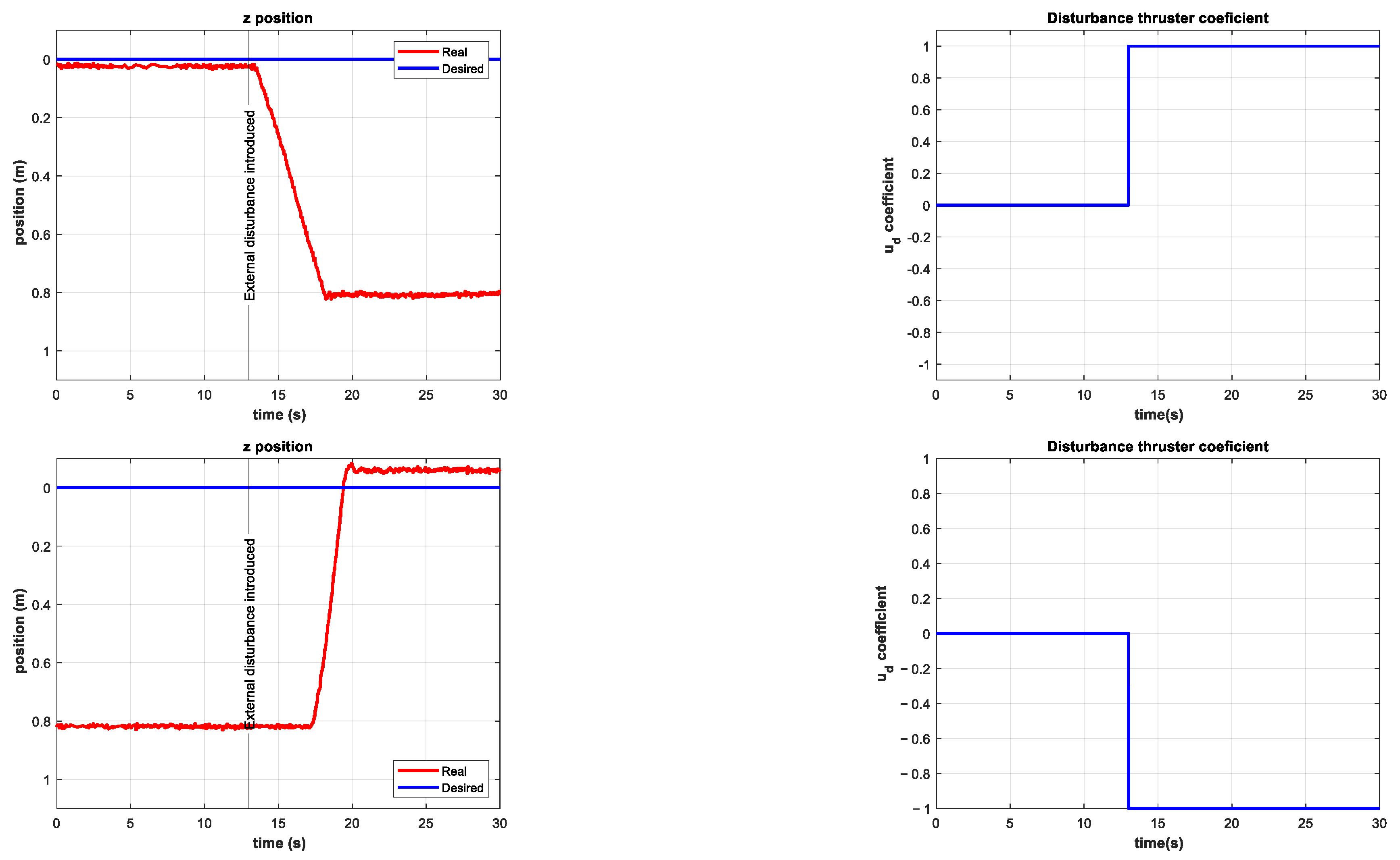
Figure 12.
Results of the open-loop experiments. Depth of the vehicle (upper left) with an external disturbance of (upper right) introduced at . Depth of the vehicle (lower left) with an external disturbance of (lower right) introduced at .
Figure 12.
Results of the open-loop experiments. Depth of the vehicle (upper left) with an external disturbance of (upper right) introduced at . Depth of the vehicle (lower left) with an external disturbance of (lower right) introduced at .
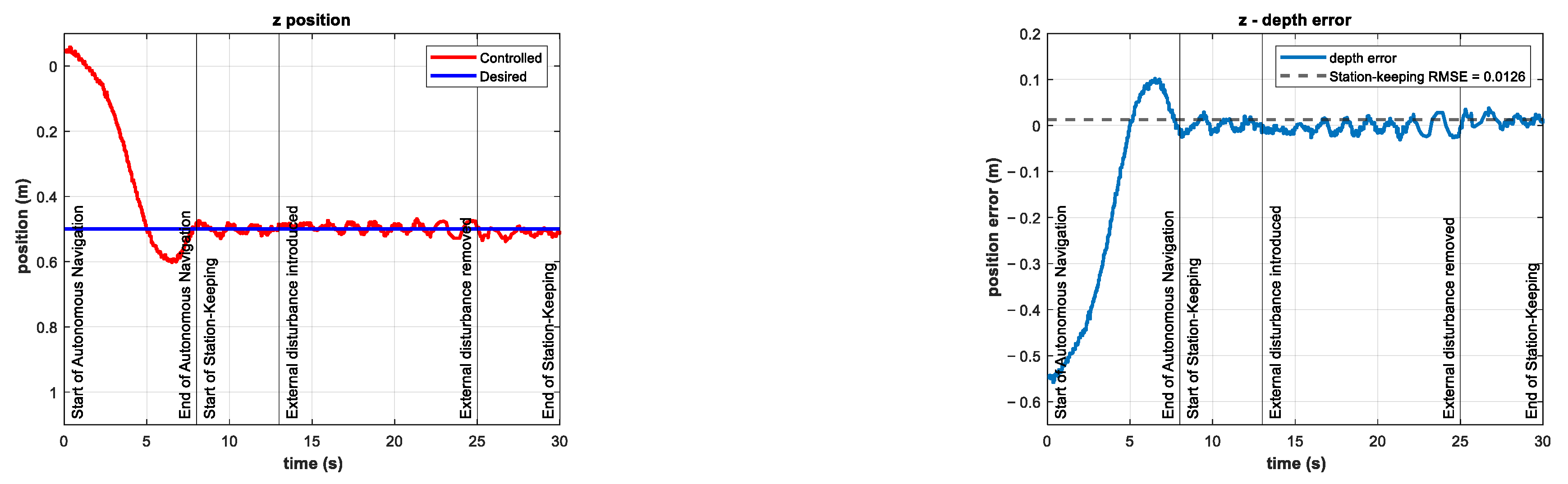
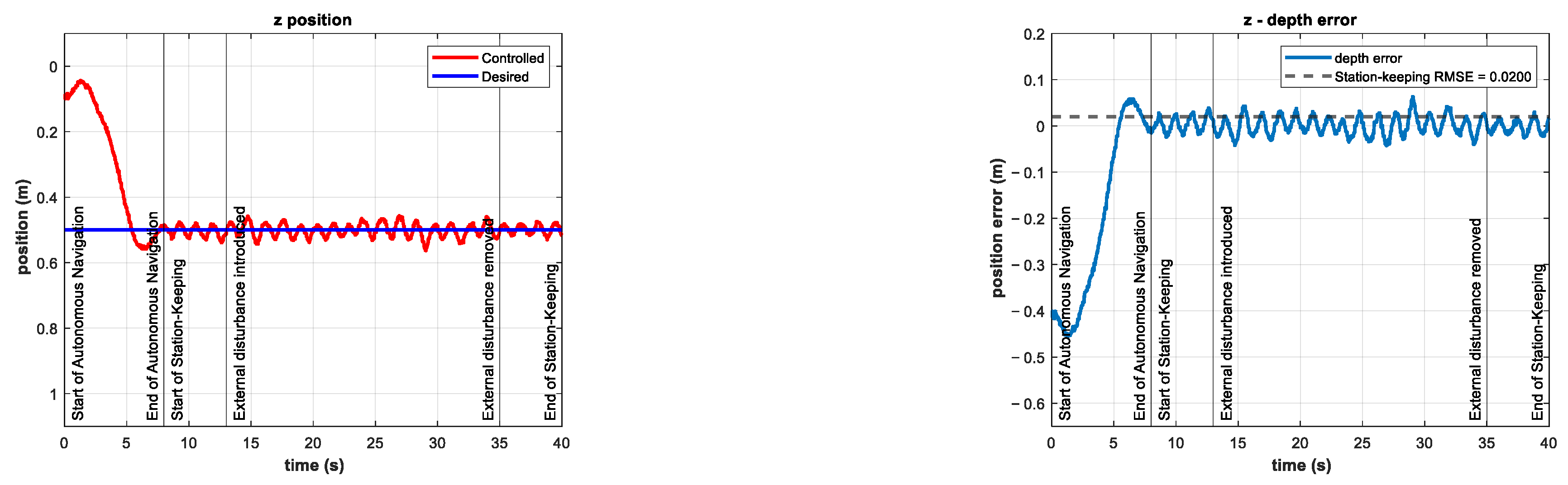
Figure 13.
Experimental results for depth station-keeping with an external disturbance of introduced in the interval . Depth (left) and tracking error (right).
Figure 13.
Experimental results for depth station-keeping with an external disturbance of introduced in the interval . Depth (left) and tracking error (right).
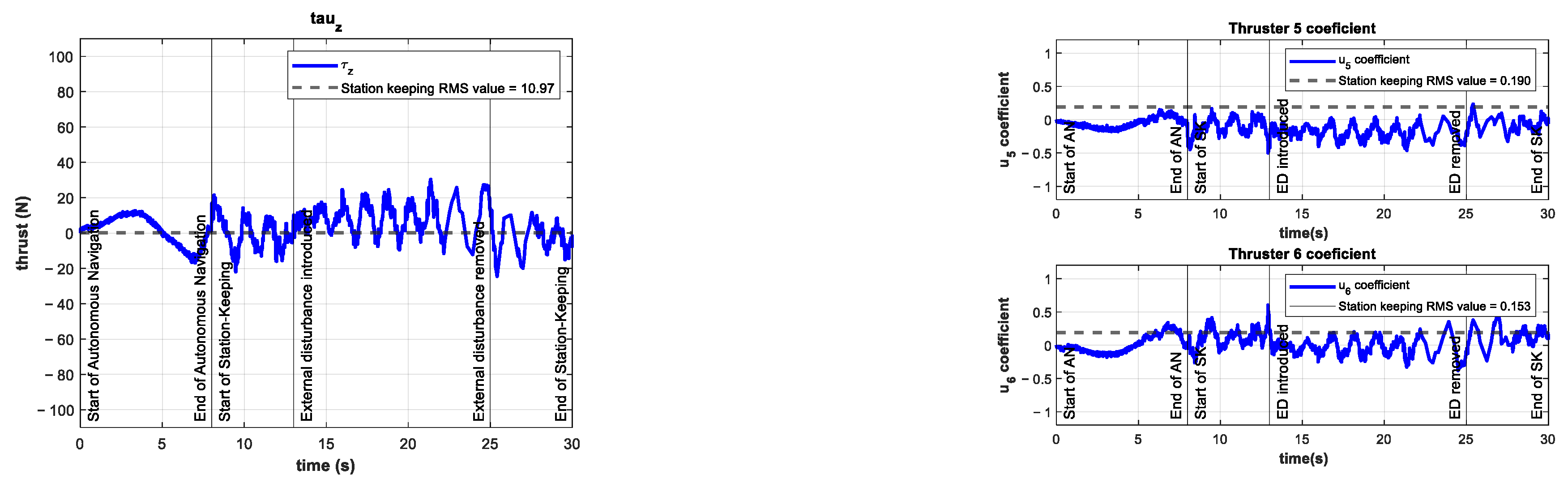
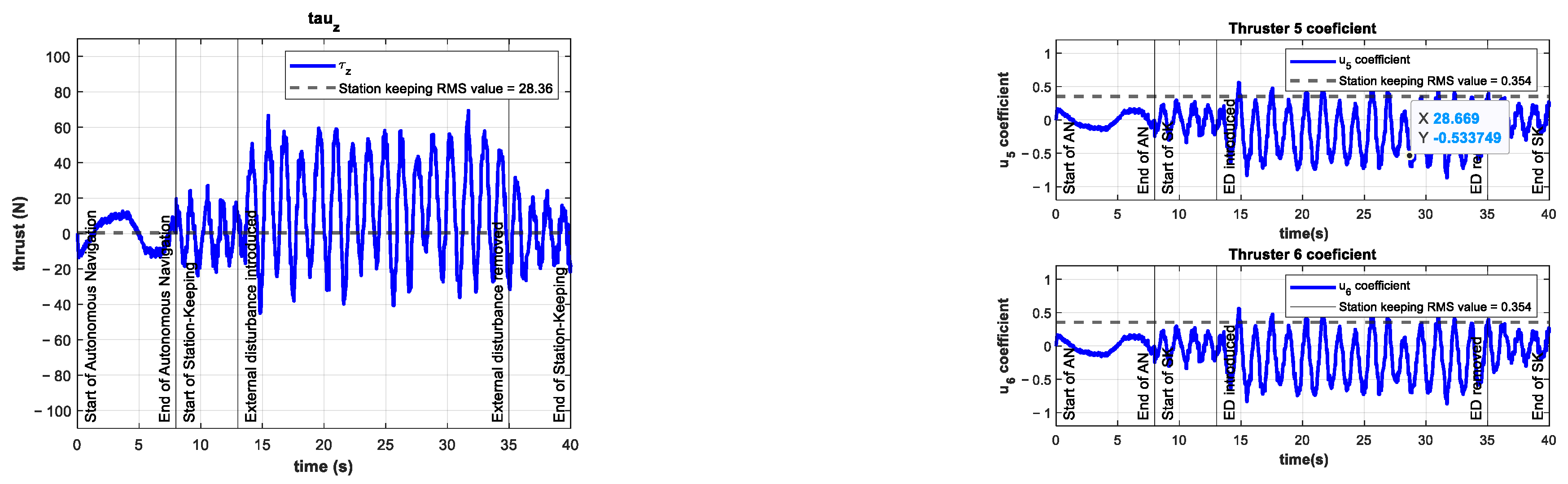
Figure 14.
Experimental results for depth station-keeping with an external disturbance of introduced in the interval . Control signal (left) and thruster coefficients , (right).
Figure 14.
Experimental results for depth station-keeping with an external disturbance of introduced in the interval . Control signal (left) and thruster coefficients , (right).
Figure 15.
Additional thruster coefficient of −0.25 in the interval .
Figure 15.
Additional thruster coefficient of −0.25 in the interval .
Figure 16.
Experimental results for depth station-keeping with an external disturbance of introduced in the interval . Depth (left) and tracking error (right).
Figure 16.
Experimental results for depth station-keeping with an external disturbance of introduced in the interval . Depth (left) and tracking error (right).
Figure 17.
Experimental results for depth station-keeping with an external disturbance of introduced in the interval . Control signal (left) and thruster coefficients , (right).
Figure 17.
Experimental results for depth station-keeping with an external disturbance of introduced in the interval . Control signal (left) and thruster coefficients , (right).
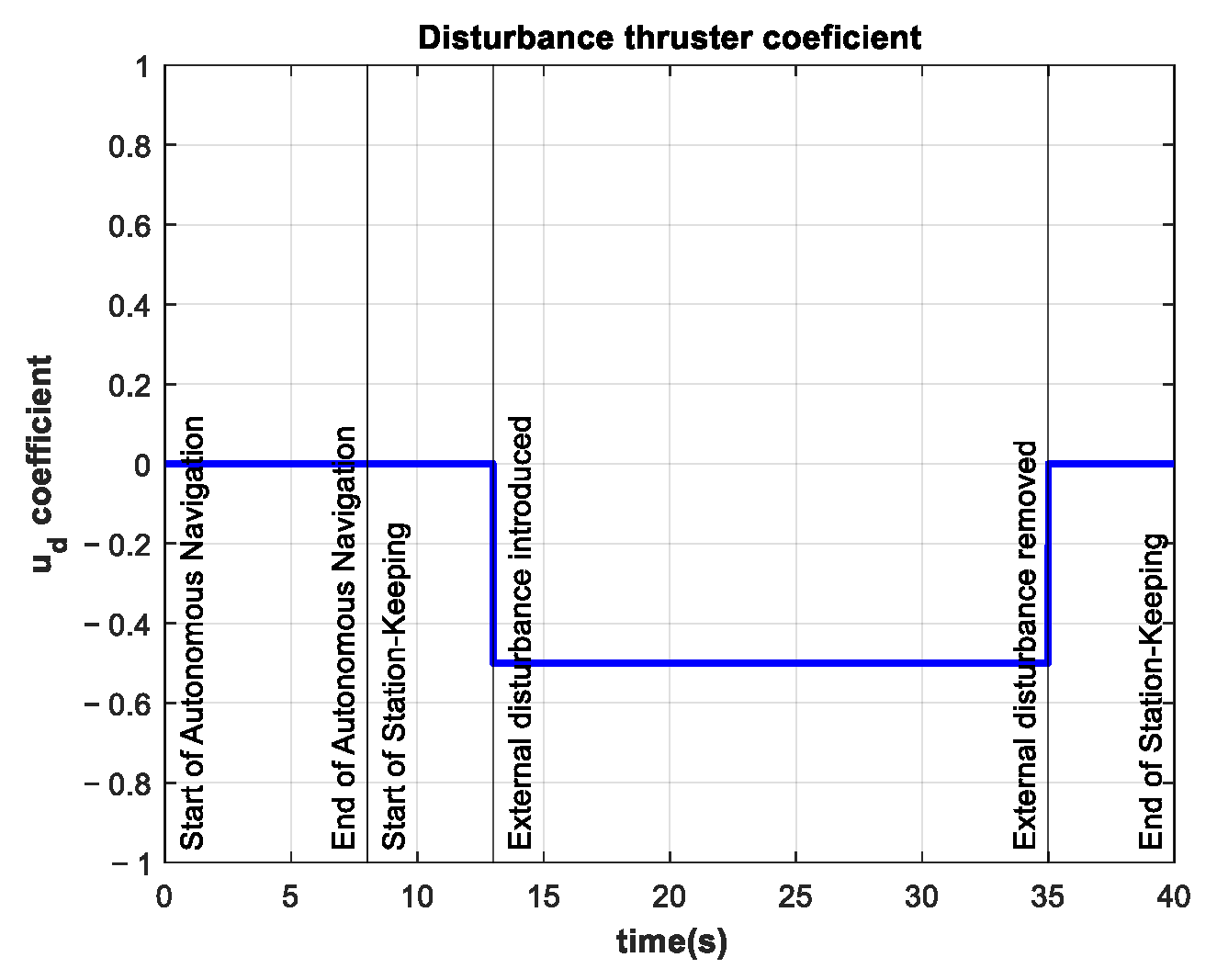
Figure 18.
Additional thruster coefficient of −0.50 in the interval .
Figure 18.
Additional thruster coefficient of −0.50 in the interval .
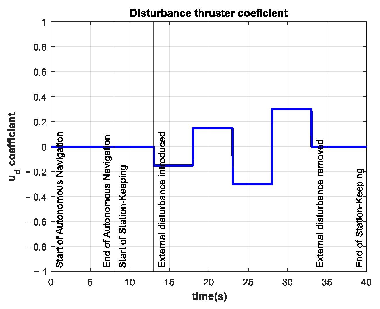
Figure 19.
Time-varying additional thruster coefficient in the interval . Minimum value −0.25 and maximum value 0.25.
Figure 19.
Time-varying additional thruster coefficient in the interval . Minimum value −0.25 and maximum value 0.25.
Figure 20.
Experimental results for depth station-keeping with a time-varying external disturbance introduced in the interval . Depth (left) and tracking error (right).
Figure 20.
Experimental results for depth station-keeping with a time-varying external disturbance introduced in the interval . Depth (left) and tracking error (right).
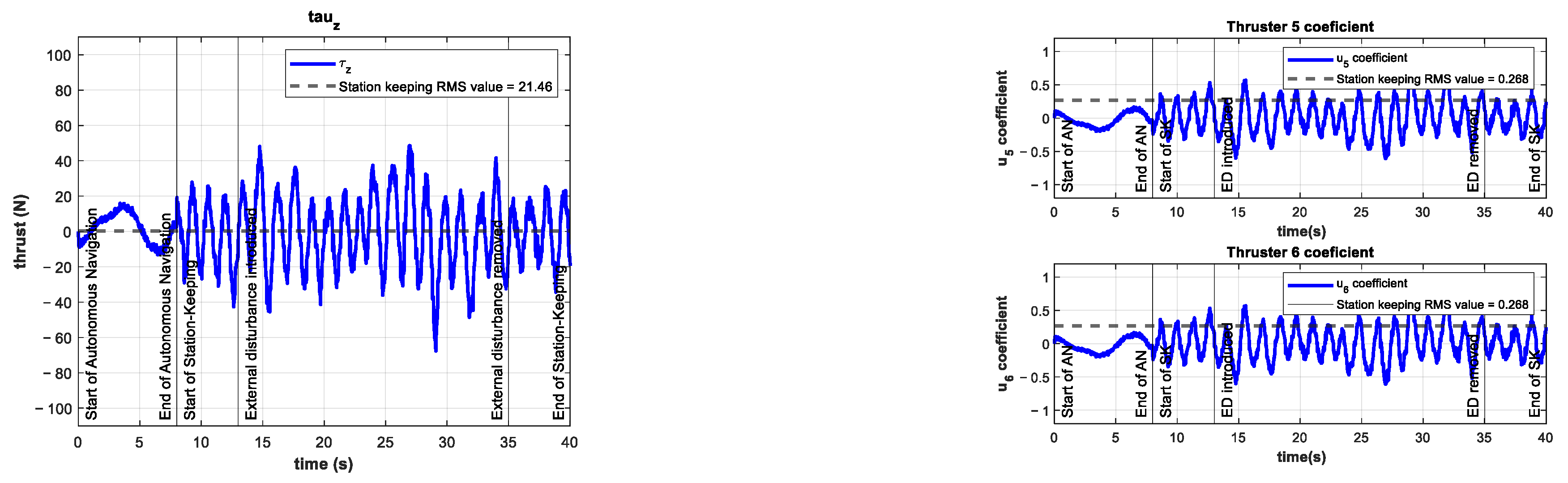
Figure 21.
Experimental results for depth station-keeping with a time-varying external disturbance introduced in the interval . Control signal (left) and thruster coefficients , (right).
Figure 21.
Experimental results for depth station-keeping with a time-varying external disturbance introduced in the interval . Control signal (left) and thruster coefficients , (right).
Table 1.
SNAME notation for underwater vehicles.
Table 1.
SNAME notation for underwater vehicles.
| Movement | Name | Position | Velocity | Force/Moment |
|---|
| X translation | Surge | | | |
| Y translation | Sway | | | |
| Z translation | Heave | | | |
| X rotation | Roll | | | |
| Y rotation | Pitch | | | |
| Z rotation | Yaw | | | |
Table 2.
Controller parameter set.
Table 2.
Controller parameter set.
| Parameter | Value | Parameter | Value |
|---|
| 0 | | 0.001 |
| 8 | | 5 |
| 1.01 | | |
| 20 | | |
Table 3.
Controller parameters for experimentation.
Table 3.
Controller parameters for experimentation.
| Parameter | Value | Parameter | Value |
|---|
| 0 | | 0.001 |
| 8 | | 5 |
| 1.005 | | 0.05 |
| 10 | | 100 |
Table 4.
Experimental results for the vertical thruster coefficients in the station-keeping phase.
Table 4.
Experimental results for the vertical thruster coefficients in the station-keeping phase.
| Experiment | | Depth RMSE (m) | Disturbance Thruster Coefficient | Thrusters’ Saturation |
|---|
| Control (C-T) | 0.1275 | 0.011 | 0.00 | No |
| 1 | 0.1609 | 0.011 | 0.15 | No |
| 2 | 0.1720 | 0.013 | 0.25 | No |
| 3 | 0.1674 | 0.012 | 0.35 | No |
| 4 | 0.3546 | 0.024 | 0.50 | No |
| 5 | 0.5877 | 0.043 | 0.75 | Yes |
| 6 | 0.5810 | 0.040 | 1.00 | Yes |
| 7 | 0.1591 | 0.010 | −0.15 | No |
| 8 | 0.1627 | 0.013 | −0.25 | No |
| 9 | 0.2397 | 0.027 | −0.35 | No |
| 10 | 0.2249 | 0.020 | −0.50 | No |
| 11 | 0.2518 | 0.017 | −0.75 | No |
| 12 | 0.3106 | 0.021 | −1.00 | No |
| 13 | 0.1453 | 0.009 | 0.15 to 0.25 | No |
| 14 | 0.1275 | 0.009 | 0.15 to 0.25 | No |
| 15 | 0.1698 | 0.012 | −0.15 to −0.25 | No |
| 16 | 0.2081 | 0.018 | −0.15 to −0.25 | No |
| 17 | 0.2683 | 0.020 | −0.35 to + 0.35 | No |
| 18 | 0.2312 | 0.017 | −0.35 to + 0.35 | No |
Table 5.
Experimental results for the control signal in the station-keeping phase.
Table 5.
Experimental results for the control signal in the station-keeping phase.
| Experiment | | % vs. C-T | Disturbance Thruster Coefficient | Thrusters’ Saturation |
|---|
| Control (C-T) | 5.88 | - | 0.00 | No |
| 1 | 8.95 | 152% | 0.15 | No |
| 2 | 10.97 | 187% | 0.25 | No |
| 3 | 11.63 | 198% | 0.35 | No |
| 4 | 28.36 | 482% | 0.50 | No |
| 5 | 49.57 | 843% | 0.75 | Yes |
| 6 | 50.18 | 853% | 1.00 | Yes |
| 7 | 7.98 | 136% | −0.15 | No |
| 8 | 9.79 | 166% | −0.25 | No |
| 9 | 16.03 | 273% | −0.35 | No |
| 10 | 14.95 | 254% | −0.50 | No |
| 11 | 20.14 | 342% | −0.75 | No |
| 12 | 25.12 | 427% | −1.00 | No |
| 13 | 10.39 | 177% | 0.15 to 0.25 | No |
| 14 | 8.81 | 150% | 0.15 to 0.25 | No |
| 15 | 10.43 | 177% | −0.15 to −0.25 | No |
| 16 | 13.64 | 232% | −0.15 to −0.25 | No |
| 17 | 21.46 | 365% | −0.35 to +0.35 | No |
| 18 | 18.50 | 314% | −0.35 to +0.35 | No |


 ,
, 


