
An Industrial Fault Diagnostic System Based on a Cubic Dynamic Uncertain Causality Graph


Abstract
:
1. Introduction
2. The Cubic DUCG Modeling and Fault-Diagnosis Method
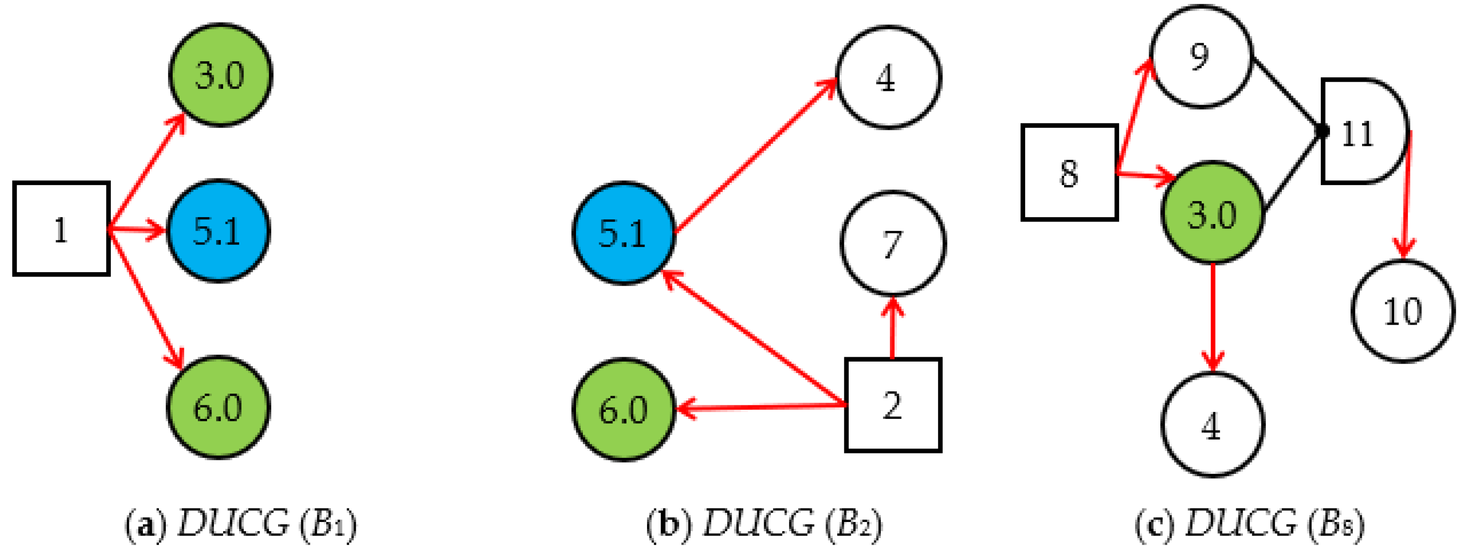
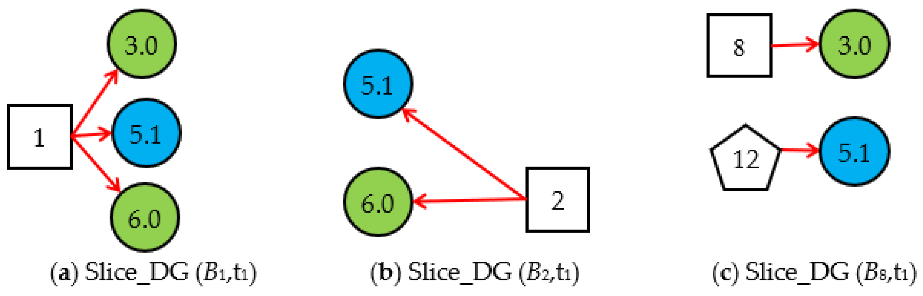
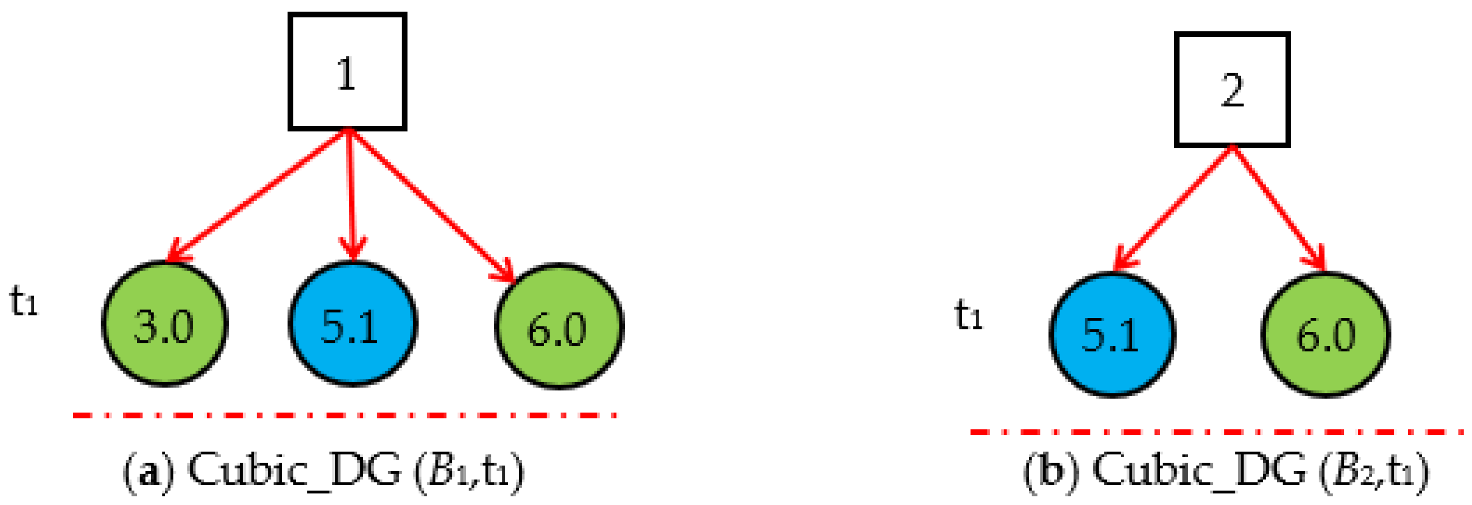
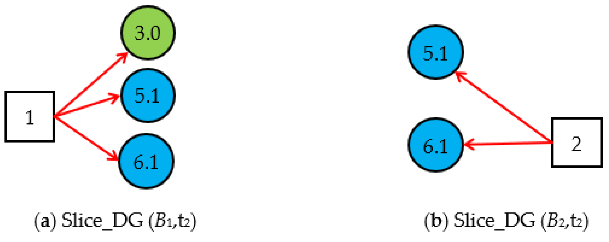
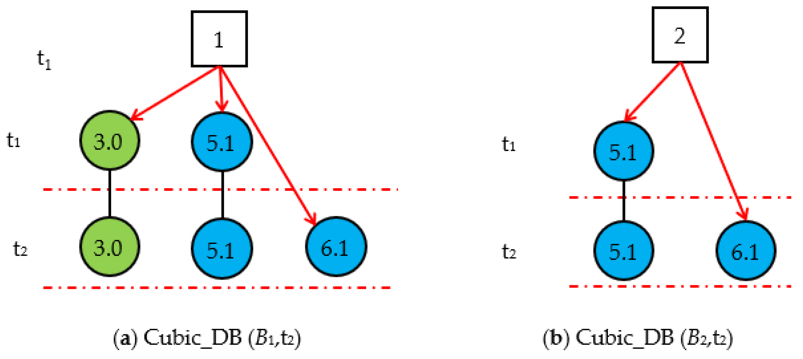
2.1. Cubic DUCG Modeling
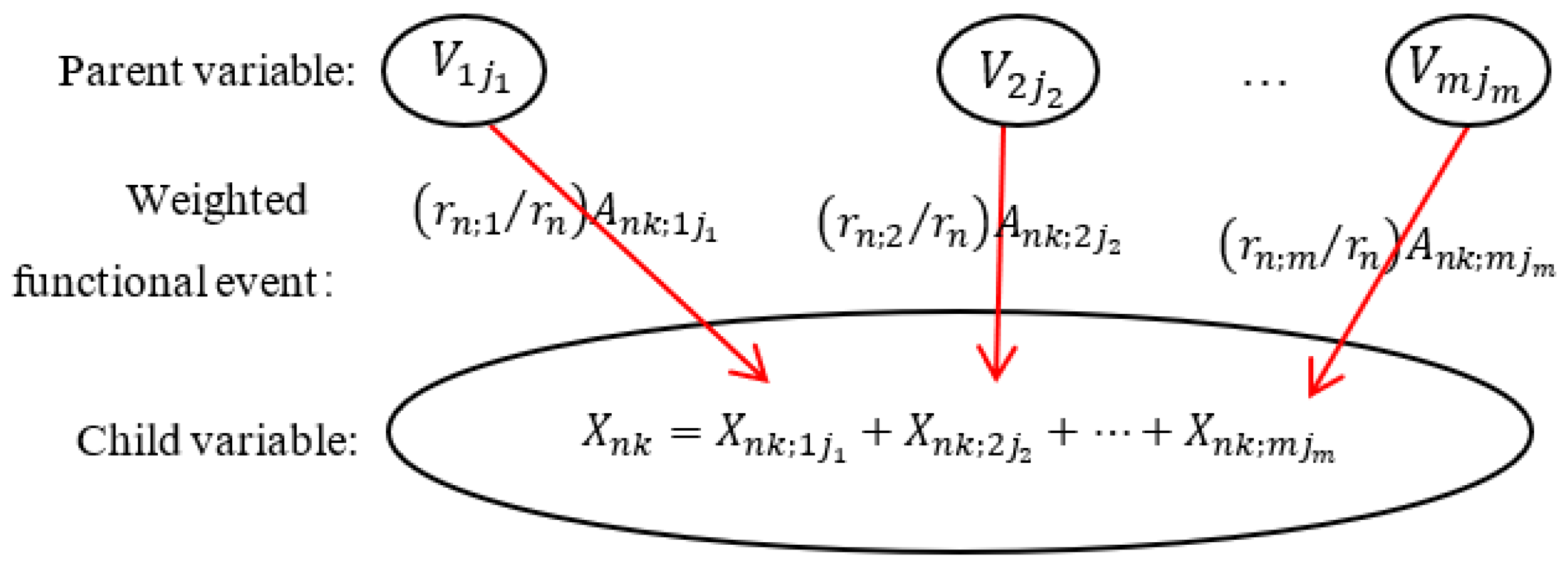
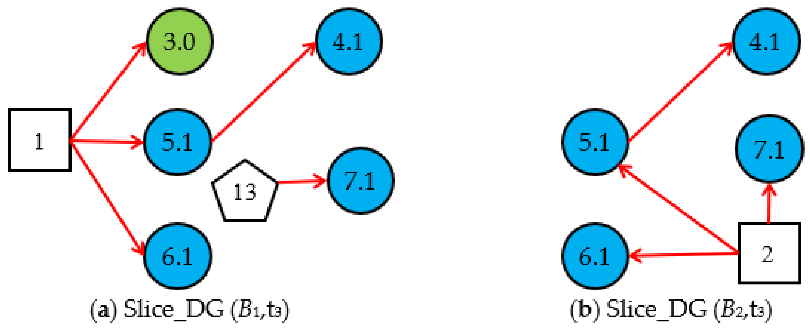
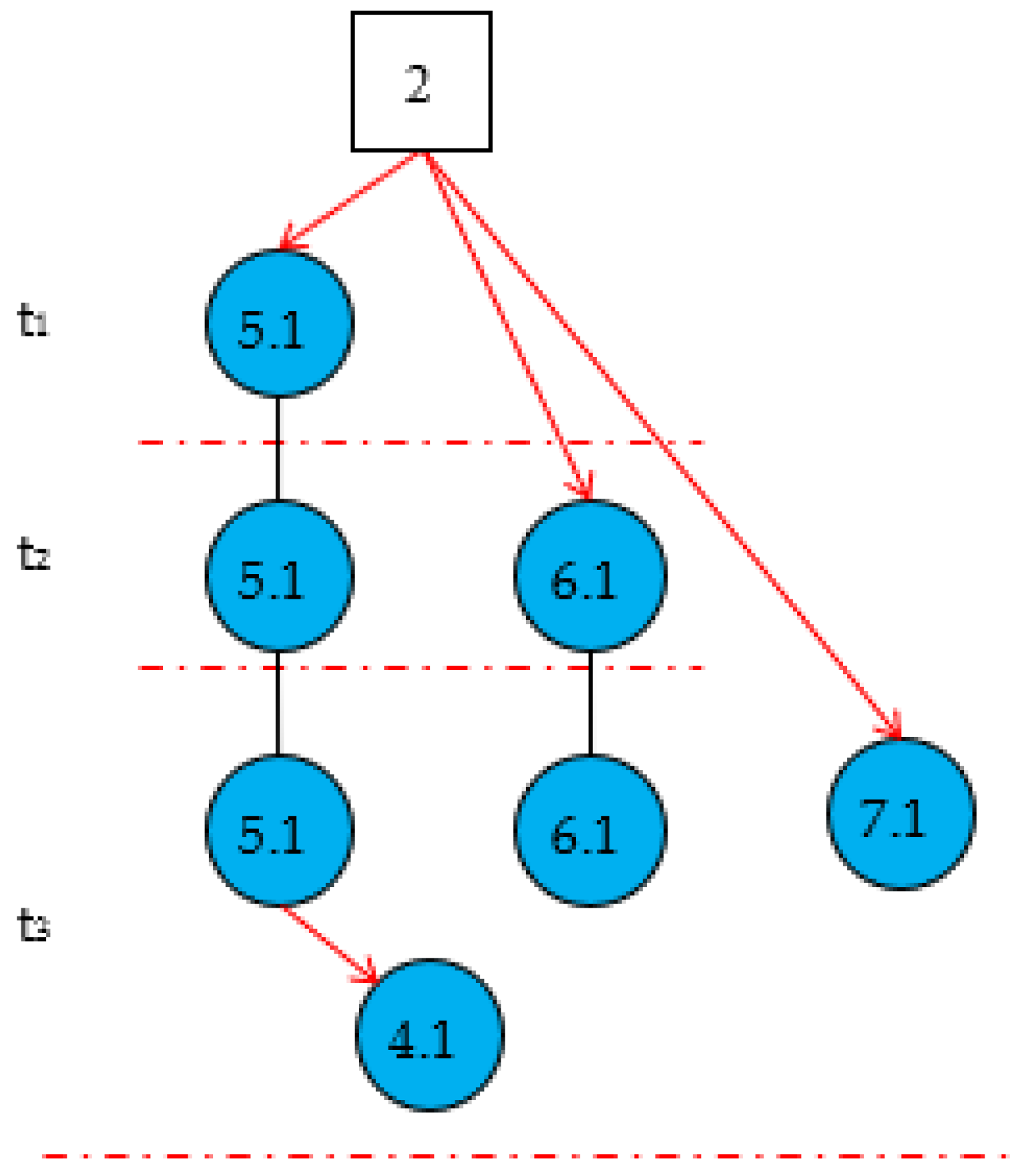
2.2. The Inference Method of the Cubic DUCG
| Algorithm 1: The Inference of the Cubic DUCG. (Note: The pseudo algorithm for inference process of the cubic DUCG.) |
| Input: the original DUCG, the evidence at time tm. Steps:
|
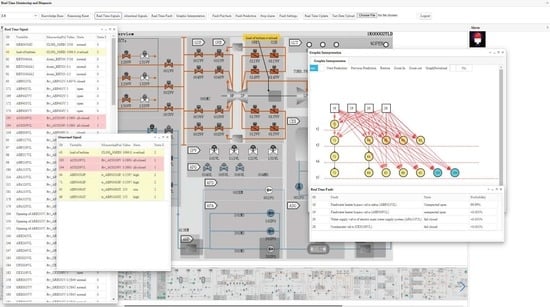
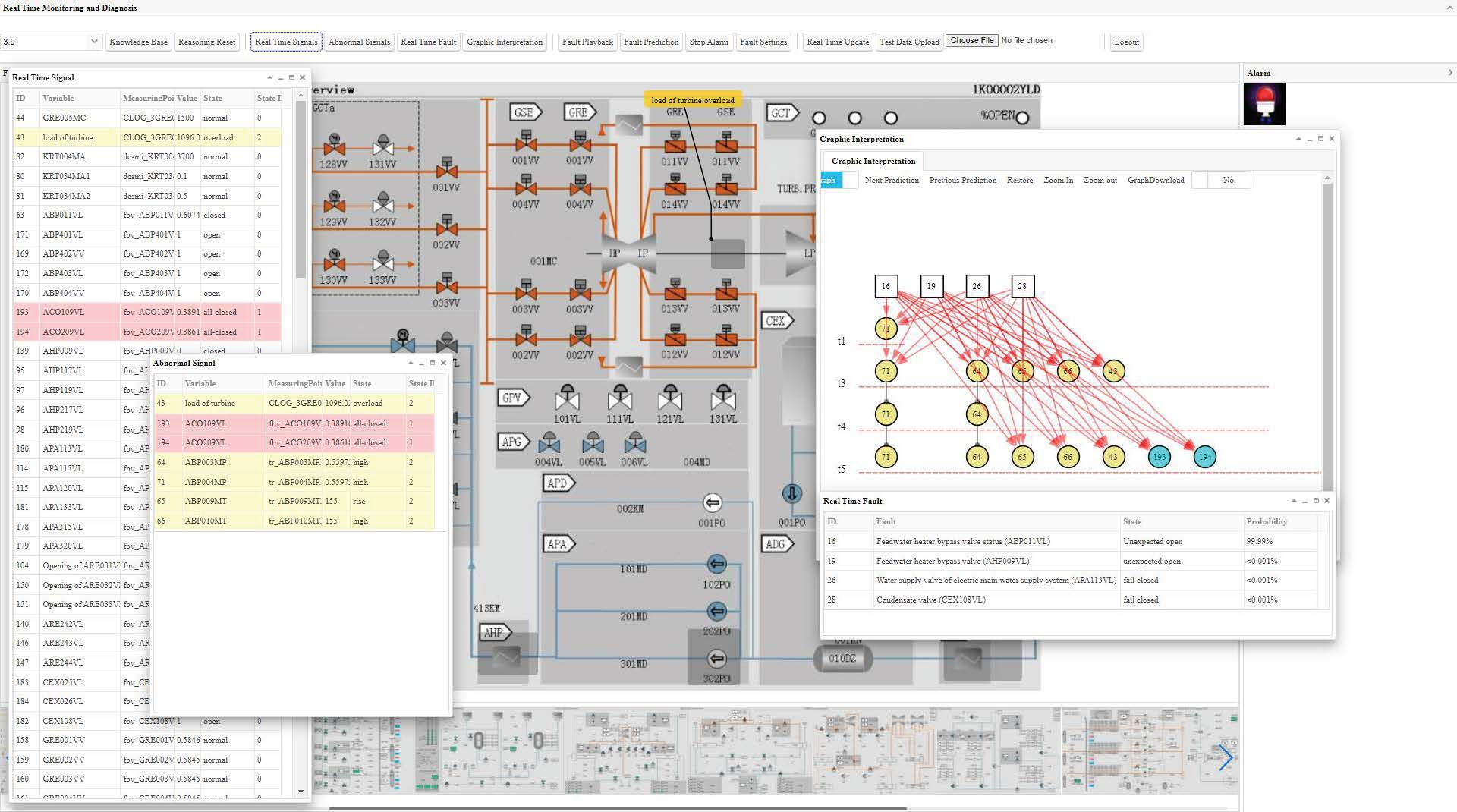
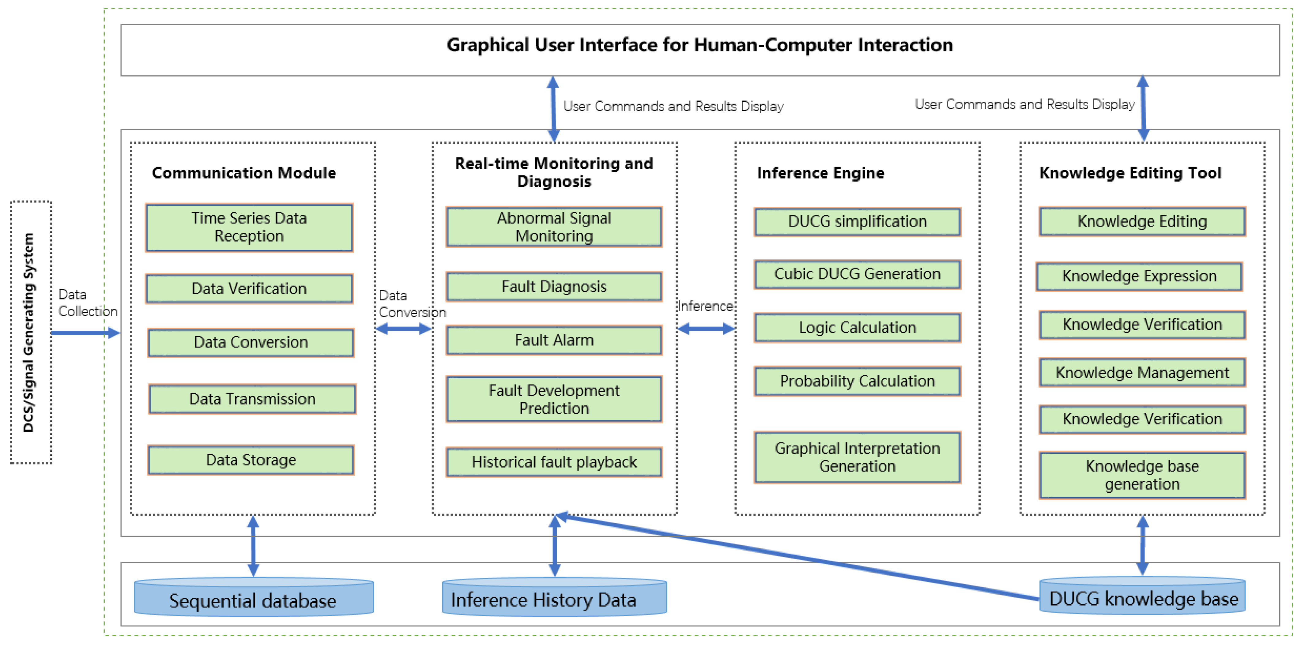
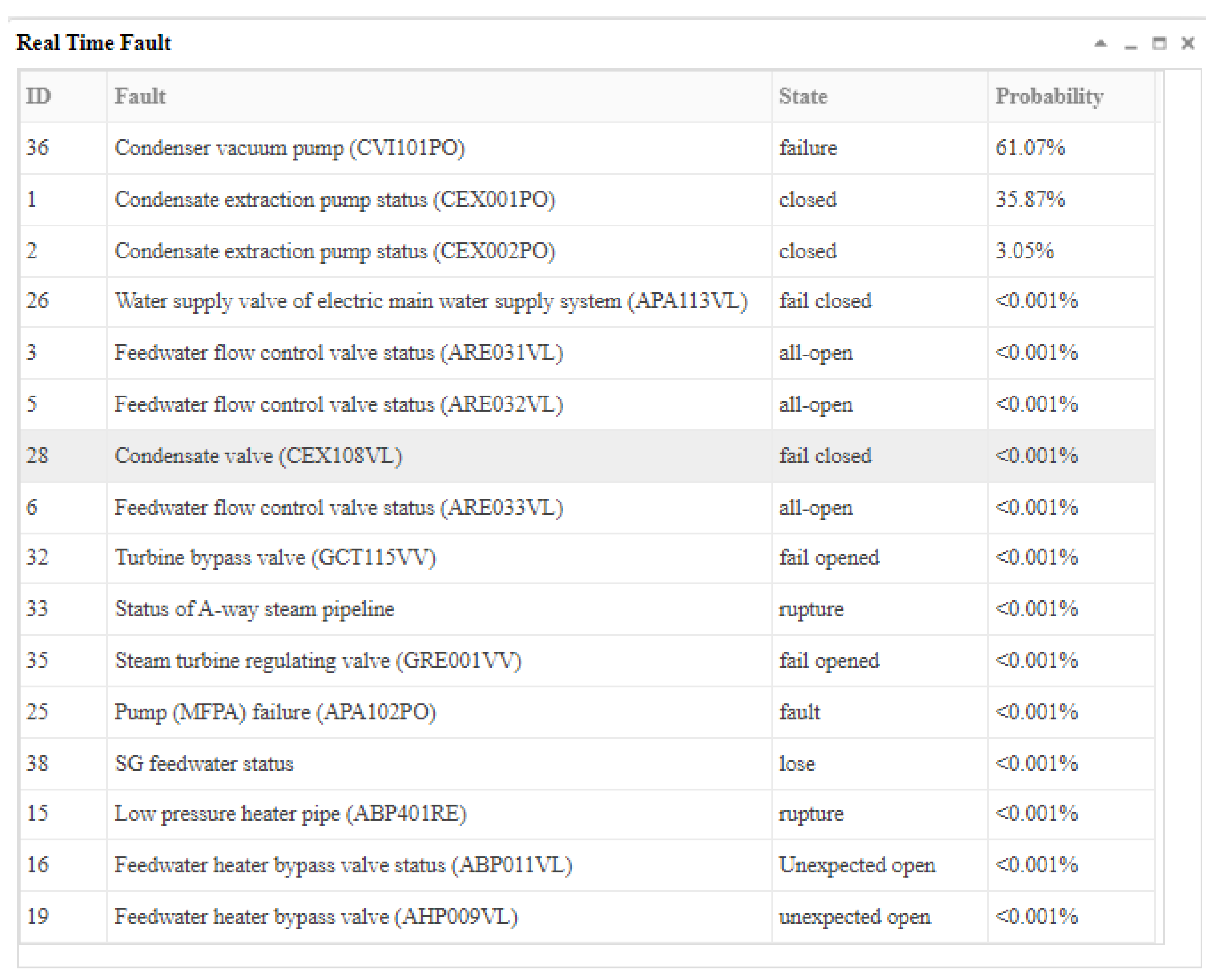
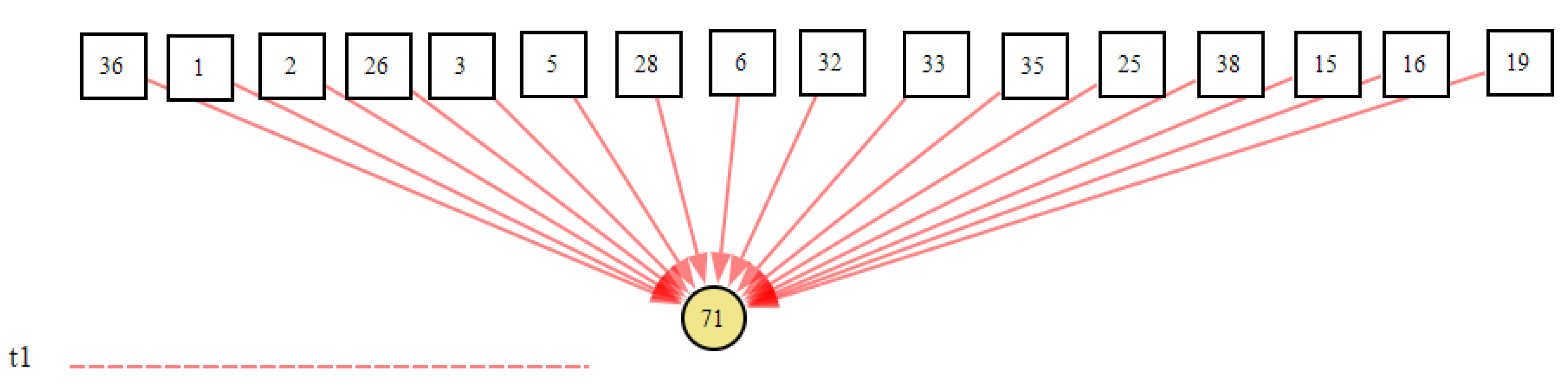
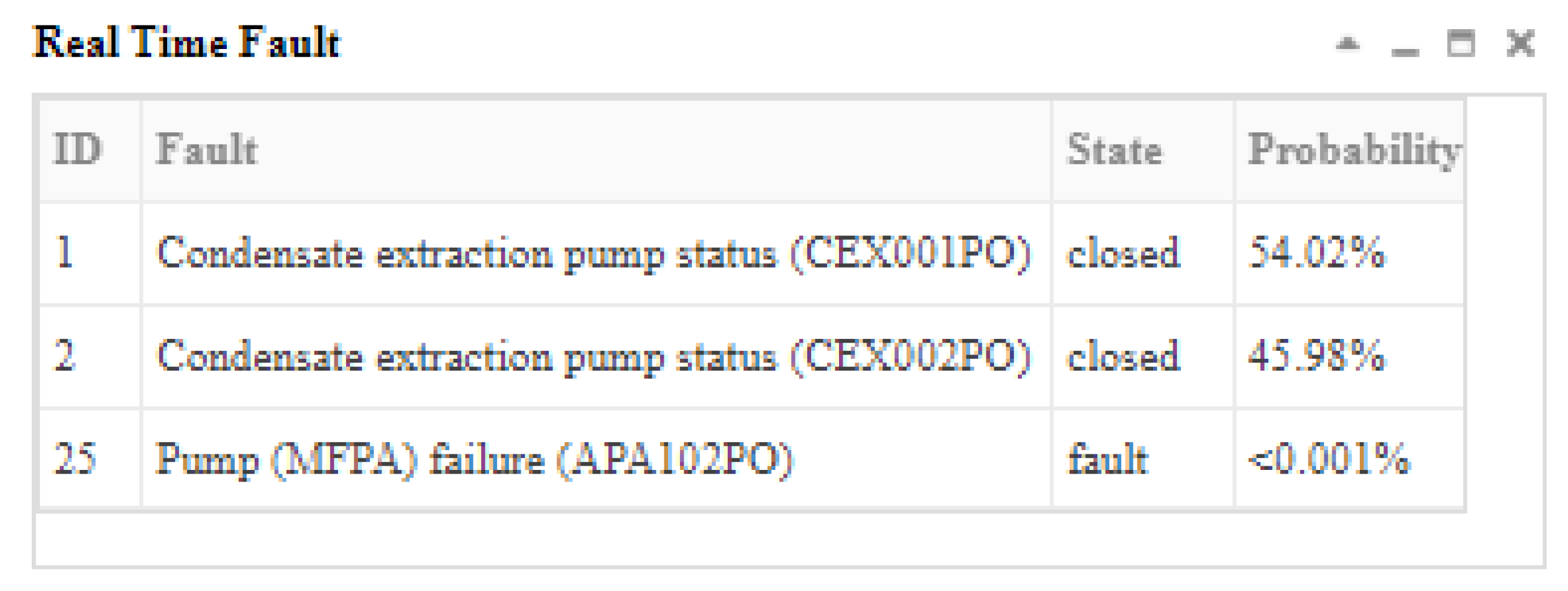
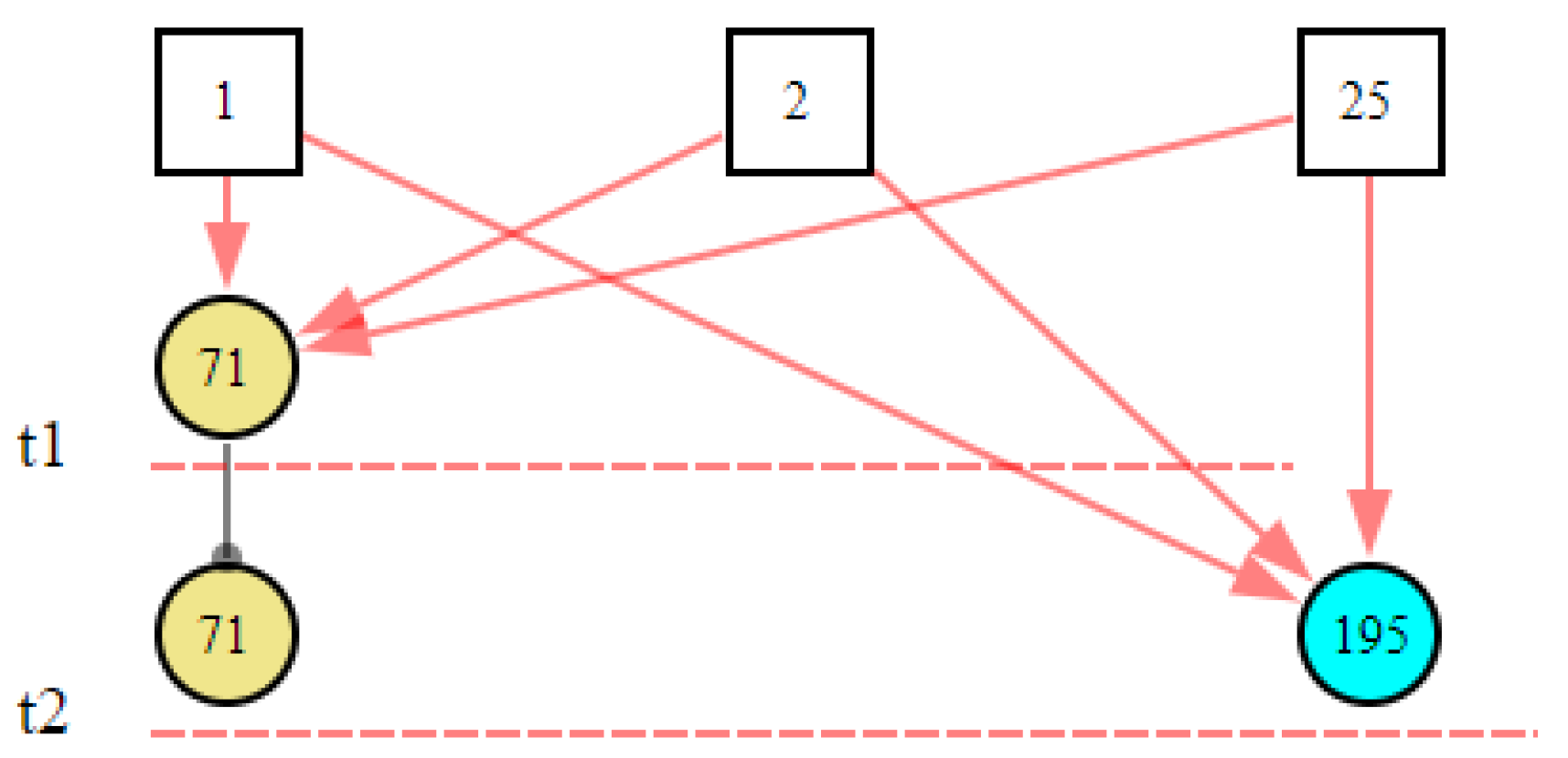
3. System Design
4. Experiment
5. Conclusions
Author Contributions
Funding
Institutional Review Board Statement
Informed Consent Statement
Data Availability Statement
Acknowledgments
Conflicts of Interest
Appendix A. The Parameters of the Example DUCG Knowledge Base
Appendix B. Description of 24 Faults in the Knowledge Base, Including Fault Name, State Description, and Its Number in DUCG

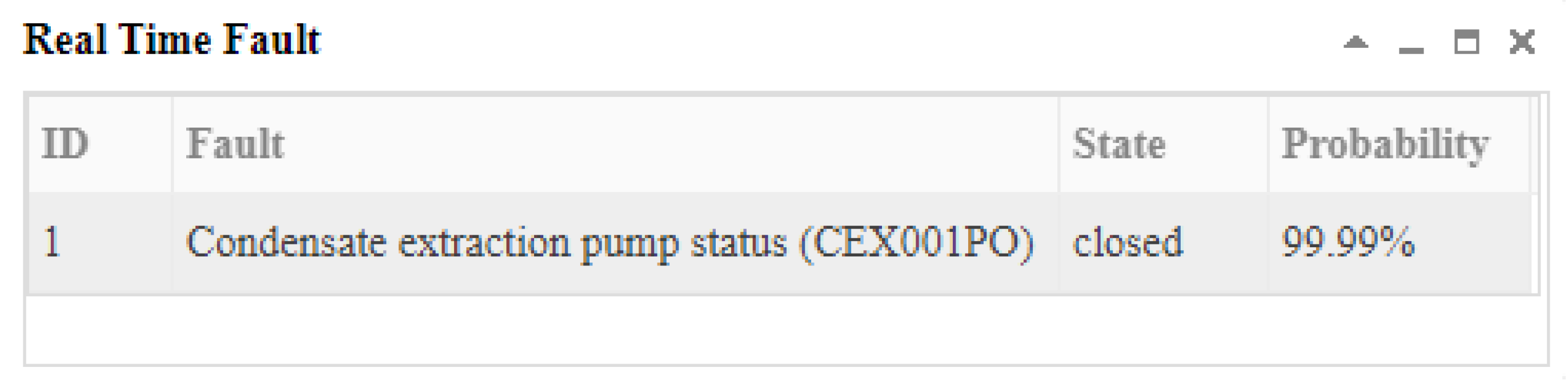
| ID | Fault Description | State | State Description |
|---|---|---|---|
| B1 | Condensate extraction pump status (CEX001PO) | 0 | Working order |
| 1 | Closed | ||
| B2 | Condensate extraction pump status (CEX002PO) | 0 | Working order |
| 1 | Closed | ||
| B3 | Feedwater flow control valve status (ARE031VL) | 0 | Normal |
| 1 | All closed | ||
| 2 | All opened | ||
| B5 | Feedwater flow control valve status (ARE032VL) | 0 | Normal |
| 1 | All closed | ||
| 2 | All opened | ||
| B6 | Feedwater flow control valve status (ARE033VL) | 0 | Normal |
| 1 | All closed | ||
| 2 | All opened | ||
| B12 | Water supply pipeline of route A | 0 | Normal |
| 1 | Leaked | ||
| B13 | Turbine operation status | 0 | Working order |
| 1 | Tripping state | ||
| B15 | Low pressure heater pipe (ABP401RE) | 0 | Normal |
| 1 | Rupture | ||
| B16 | Feedwater heater bypass valve status (ABP011VL) | 0 | Normal |
| 1 | Accidental opening | ||
| B17 | Main steam header status | 0 | Normal |
| 1 | Leaked | ||
| B18 | Steam generator heat transfer tube | 0 | Normal |
| 1 | Leaked | ||
| B19 | Feedwater heater bypass valve (AHP009VL) | 0 | Normal |
| 1 | Accidental opening | ||
| B20 | Water supply pipeline of route B | 0 | Normal |
| 1 | Leaked | ||
| B21 | Water supply pipeline of route C | 0 | Normal |
| 1 | Leaked | ||
| B25 | Pump (MFPA) failure (APA102PO) | 0 | Normal |
| 1 | Fault condition | ||
| B26 | Water supply valve of electric main water supply system (APA113VL) | 0 | Normal |
| 1 | Accidental shutdown | ||
| B28 | Water supply valve of electric main water supply system (APA113VL) | 0 | Normal |
| 1 | Accidental shutdown | ||
| B32 | Turbine bypass valve (GCT115VV) | 0 | Normal |
| 1 | Accidental opening | ||
| B33 | Status of A-way steam pipeline | 0 | Normal |
| 1 | Rupture | ||
| B34 | Turbine bypass valve (GCT131VV) | 0 | Normal |
| 1 | Accidental opening | ||
| B35 | Steam turbine regulating valve (GRE001VV) | 0 | Normal |
| 1 | Accidental all closed | ||
| 2 | Accidental all opened | ||
| B36 | Condenser vacuum pump (CVI101PO) | 0 | Normal |
| 1 | Accidental failure | ||
| B37 | Status of three main steam isolation valves (VVP001/002/003VV) | 0 | Normal |
| 1 | All closed | ||
| B38 | SG feedwater status | 0 | Normal |
| 1 | Loss | ||
| 2 | Moderate |
References
- Fernandes, M.; Corchado, J.M.; Marreiros, G. Machine learning techniques applied to mechanical fault diagnosis and fault prognosis in the context of real industrial manufacturing use-cases: A systematic literature review. Appl. Intell. 2022, 1–35. [Google Scholar] [CrossRef] [PubMed]
- Liu, G.; Shen, W.; Gao, L.; Kusiak, A. Knowledge transfer in fault diagnosis of rotary machines. IET Collab. Intell. Manuf. 2022, 4, 17–34. [Google Scholar] [CrossRef]
- Hongm, W.; Tian-You, C.; Jin-Liang, D.; Brown, M. Data Driven Fault Diagnosis and Fault Tolerant Control: Some Advances and Possible New Directions. Acta Autom. Sin. 2009, 35, 739–747. [Google Scholar] [CrossRef] [Green Version]
- Nasser, A.R.; Azar, A.T.; Humaidi, A.J.; Al-Mhdawi, A.K.; Ibraheem, I.K. Intelligent Fault Detection and Identification Approach for Analog Electronic Circuits Based on Fuzzy Logic Classifier. Electronics 2021, 10, 2888. [Google Scholar] [CrossRef]
- He, Y.L.; Ma, Y.; Xu, Y.; Zhu, Q.X. Fault Diagnosis Using Novel Class-Specific Distributed Monitoring Weighted Nave Bayes: Applications to Process Industry. Ind. Eng. Chem. Res. 2020, 59, 9593–9603. [Google Scholar] [CrossRef]
- Estima, J.O.; Cardoso, A. A New Approach for Real-Time Multiple Open-Circuit Fault Diagnosis in Voltage Source Inverters. IEEE Trans. Ind. Appl. 2011, 47, 2487–2494. [Google Scholar] [CrossRef]
- Wang, J.; Wang, F.; Chen, S.; Wang, J.; Hu, L.; Yin, Y.; Wu, Y. Fault-tree-based instantaneous risk computing core in nuclear power plant risk monitor. Ann. Nucl. Energy 2016, 95, 35–41. [Google Scholar] [CrossRef]
- Rojas-Guzman, C.; Kramer, M.A. Comparison of belief networks and rule-based expert systems for fault diagnosis of chemical processes. Eng. Appl. Artif. Intell. 1993, 6, 191–202. [Google Scholar] [CrossRef]
- Grant, P.W.; Harris, P.M.; Moseley, L.G. Fault diagnosis for industrial printers using case-based reasoning. Eng. Appl. Artif. Intell. 1996, 9, 163–173. [Google Scholar] [CrossRef]
- Mustapha, F.; Sapuan, S.M.; Ismail, N.; Mokhtar, A.S. A computer-based intelligent system for fault diagnosis of an aircraft engine. Eng. Comput. 2004, 21, 78–90. [Google Scholar] [CrossRef]
- Nan, C.; Khan, F.; Iqbal, M.T. Real-time fault diagnosis using knowledge-based expert system. Process Saf. Environ. Prot. 2008, 86, 55–71. [Google Scholar] [CrossRef]
- Bernard, J.A. Use of a rule-based system for process control. IEEE Control Syst. Mag. 1987, 8, 3–13. [Google Scholar] [CrossRef]
- Geus, A.J.D.; Cohen, W. A Rule-Based System for Optimizing Combinational Logic. IEEE Des. Test Comput. 1985, 2, 22–32. [Google Scholar] [CrossRef]
- You, D.; Gao, X.; Katayama, S. WPD-PCA-based laser welding process monitoring and defects diagnosis by using FNN and SVM. IEEE Trans. Ind. Electron. 2015, 62, 628–636. [Google Scholar] [CrossRef]
- Chiang, L.H.; Kotanchek, M.E.; Kordon, A.K. Fault diagnosis based on Fisher discriminant analysis and support vector machines. Comput. Chem. Eng. 2004, 28, 1389–1401. [Google Scholar] [CrossRef]
- He, S.; Liu, X.; Wang, Y.; Xu, S.; Lu, J.; Yang, C.; Zhou, S.; Sun, Y.; Gui, W.; Qin, W. An effective fault diagnosis approach based on optimal weighted least squares support vector machine. Can. J. Chem. Eng. 2017, 95, 2357–2366. [Google Scholar] [CrossRef]
- Malik, H.; Ashish, Y.; Kumar, S.A. EMD and ANN based intelligent model for bearing fault diagnosis. J. Intell. Fuzzy Syst. 2018, 35, 5391–5402. [Google Scholar] [CrossRef]
- Wang, Z.; Liu, Y.; Griffin, P.J. A combined ANN and expert system tool for transformer fault diagnosis. IEEE Trans. Power Deliv. 2000, 13, 1224–1229. [Google Scholar] [CrossRef]
- Han, T.; Liu, C.; Yang, W.; Jiang, D. Deep Transfer Network with Joint Distribution Adaptation: A New Intelligent Fault Diagnosis Framework for Industry Application. ISA Trans. 2018, 97, 269–281. [Google Scholar] [CrossRef] [Green Version]
- Khorram, A.; Khalooei, M.; Rezghi, M. End-to-end CNN+LSTM deep learning approach for bearing fault diagnosis. Appl. Intell. 2021, 51, 736–751. [Google Scholar] [CrossRef]
- Talebi, N.; Sadrnia, M.A.; Darabi, A. Robust Fault Detection of Wind Energy Conversion Systems Based on Dynamic Neural Networks. Comput. Intell. Neurosci. 2014, 2014, 580972. [Google Scholar] [CrossRef] [PubMed] [Green Version]
- Zhao, X.; Jia, M.; Bin, J.; Wang, T.; Liu, Z. Multiple-Order Graphical Deep Extreme Learning Machine for Unsupervised Fault Diagnosis of Rolling Bearing. IEEE Trans. Instrum. Meas. 2020, 70, 3506012. [Google Scholar] [CrossRef]
- Vaddi, P.K.; Pietrykowski, M.C.; Kar, D.; Diao, X.; Zhao, Y.; Mabry, T.; Ray, I.; Smidts, C. Dynamic bayesian networks based abnormal event classifier for nuclear power plants in case of cyber security threats. Prog. Nucl. Energy 2020, 128, 103479. [Google Scholar] [CrossRef]
- Feng, L.; Zhao, C. Fault Description Based Attribute Transfer for Zero-Sample Industrial Fault Diagnosis. IEEE Trans. Ind. Inform. 2020, 17, 1852–1862. [Google Scholar] [CrossRef]
- Martin, T.P.; Glasgow, J.I.; Féret, M.; Kelley, T. A Knowledge-Based System for Fault Diagnosis in Real-Time Engineering Applications; Springer: Vienna, Austria, 1991. [Google Scholar] [CrossRef]
- Dong, C.; Zhang, Q. The Cubic Dynamic Uncertain Causality Graph: A Methodology for Temporal Process Modeling and Diagnostic Logic Inference. IEEE Trans. Neural Netw. Learn. Syst. 2020, 31, 4239–4253. [Google Scholar] [CrossRef] [PubMed]
- Zhang, Q. Dynamic Uncertain Causality Graph for Knowledge Representation and Reasoning: Discrete DAG Cases. J. Comput. Sci. Technol. 2012, 27, 3–25. [Google Scholar] [CrossRef]
- Zhang, Q. Dynamic Uncertain Causality Graph for Knowledge Representation and Probabilistic Reasoning: Directed Cyclic Graph and Joint Probability Distribution. IEEE Trans. Neural Netw. Learn. Syst. 2015, 26, 1503–1517. [Google Scholar] [CrossRef]
- Zhang, Q. Dynamic Uncertain Causality Graph for Knowledge Representation and Reasoning: Continuous Variable, Uncertain Evidence, and Failure Forecast. IEEE Trans. Syst. Man Cybern. Syst. 2017, 45, 990–1003. [Google Scholar] [CrossRef]
- Qin, Z.; Zhan, Z. Dynamic Uncertain Causality Graph Applied to Dynamic Fault Diagnoses and Predictions with Negative Feedbacks. IEEE Trans. Reliab. 2016, 65, 1030–1044. [Google Scholar] [CrossRef]
- Zhang, Q.; Dong, C.; Cui, Y.; Yang, Z. Dynamic Uncertain Causality Graph for Knowledge Representation and Probabilistic Reasoning: Statistics Base, Matrix, and Application. IEEE Trans. Neural Netw. Learn. Syst. 2014, 25, 645. [Google Scholar] [CrossRef]
- Zhang, Q.; Yao, Q. Dynamic Uncertain Causality Graph for Knowledge Representation and Reasoning: Utilization of Statistical Data and Domain Knowledge in Complex Cases. IEEE Trans. Neural Netw. Learn. Syst. 2018, 29, 1637–1651. [Google Scholar] [CrossRef] [PubMed]
- Dong, C.L.; Zhang, Q. Research on weighted logical inference for uncertain fault diagnosis. Acta Autom. Sin. 2014, 40, 2766–2781. [Google Scholar] [CrossRef]
- Dong, C.; Zhou, Z.; Qin, Z. Cubic dynamic uncertain causality graph: A new methodology for modeling and reasoning about complex faults with negative feedbacks. IEEE Trans. Reliab. 2018, 67, 920–932. [Google Scholar] [CrossRef]
- Zhao, Y. Research on DUCG Theory and Application for Fault Diagnosis and Procedure Improvement of Nuclear Power Plant. Ph.D. Thesis, Tsinghua University, Beijing, China, 2017. [Google Scholar]


| Type | Shape | Description |
|---|---|---|
| Bi |  | The B-type variable is the root-cause variable used to represent the root cause/fault that causes other variables to occur. |
| Xi |  | The X-type variable is the consequence or process variable used to represent the result caused by the root-cause variable, and can also be used as the cause of other variables. |
| Gi |  | The G-type variable is the logic-gate variable. It is used to describe the logical relation combination of parent variables. |
| Di |  | The D-type variable is the unknown cause or default-cause variable. When the cause of a variable’s occurrence is unknown, then the D-type variable is used to represent the root cause that causes it to occur. |
| Fi;j |  | The F-type variable is the weighted functional-event variable. It is used to represent and quantify the causalities between parent variables and child variables. |
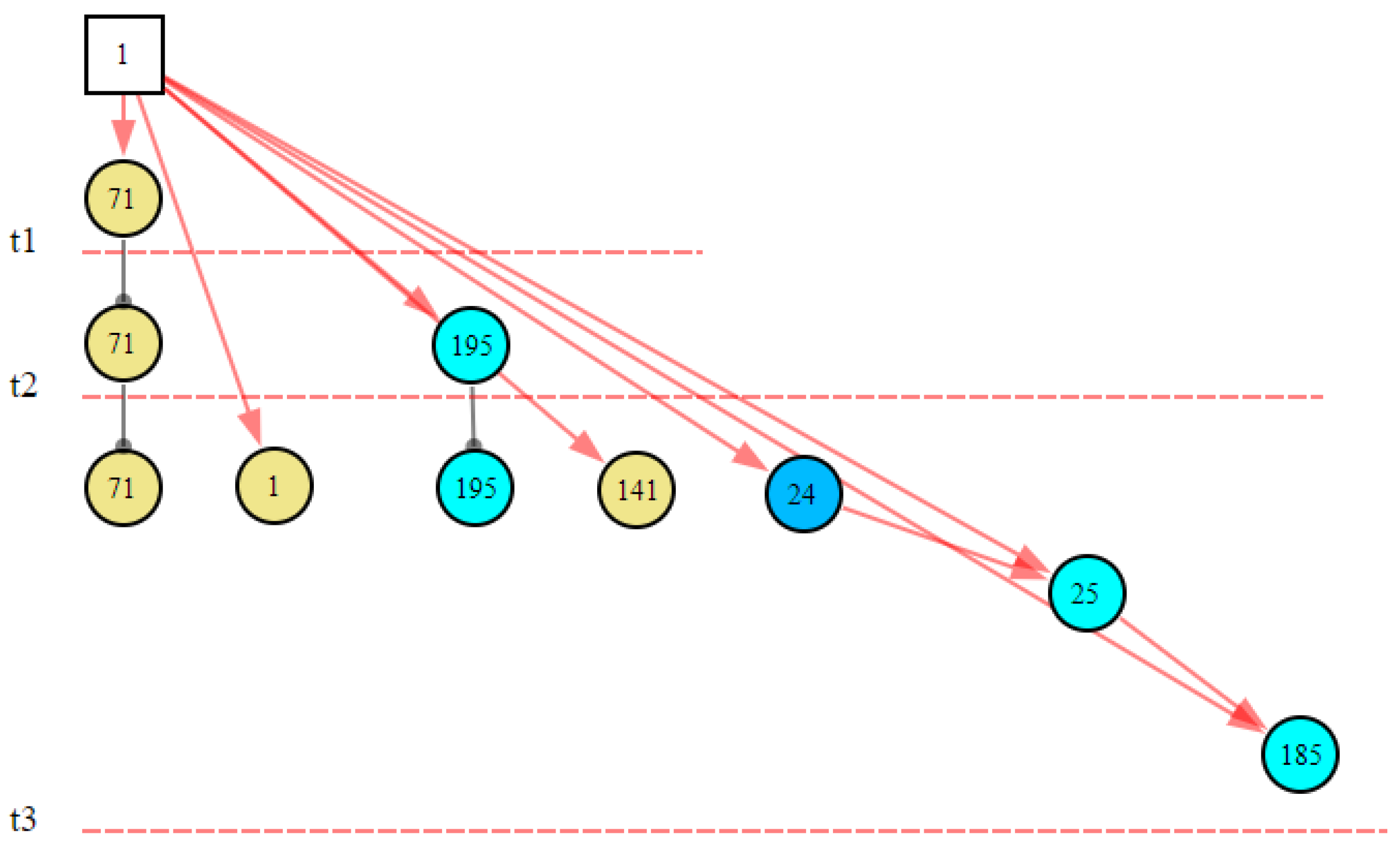
| Fault | Rank First | Confirmed Diagnosis | Time Consumption | Average Time |
|---|---|---|---|---|
| B1,1 | t2 | t3 | 145 ms | 48 ms |
| B2,1 | t1 | t1 | 19 ms | 19 ms |
| B3,2 | t1 | t1 | 18 ms | 18 ms |
| B5,2 | t1 | t1 | 19 ms | 19 ms |
| B6,2 | t1 | t1 | 18 ms | 18 ms |
| B13,1 | t1 | t1 | 313 ms | 313 ms |
| B15,1 | t1 | t1 | 26 ms | 26 ms |
| B16,1 | t3 | t8 | 437 ms | 55 ms |
| B17,1 | t1 | t1 | 21 ms | 21 ms |
| B18,1 | t1 | t1 | 20 ms | 20 ms |
| B19,1 | t3 | t8 | 433 ms | 55 ms |
| B20,1 | t1 | t1 | 274 ms | 274 ms |
| B21,1 | t1 | t1 | 276 ms | 276 ms |
| B25,1 | t1 | t1 | 81 ms | 81 ms |
| B26,1 | t2 | t2 | 188 ms | 94 ms |
| B28,1 | t1 | t1 | 23 ms | 23 ms |
| B32,1 | t1 | t1 | 142 ms | 142 ms |
| B33,1 | t1 | t1 | 230 ms | 230 ms |
| B34,1 | t4 | t4 | 496 ms | 124 ms |
| B35,1 | t1 | t12 | 1874 ms | 157 ms |
| B35,2 | t1 | t1 | 31 ms | 31 ms |
| B36,1 | t1 | t1 | 18 ms | 18 ms |
| B37,1 | t1 | t1 | 21 ms | 21 ms |
| B38,1 | t2 | t2 | 398 ms | 199 ms |
Publisher’s Note: MDPI stays neutral with regard to jurisdictional claims in published maps and institutional affiliations. |
© 2022 by the authors. Licensee MDPI, Basel, Switzerland. This article is an open access article distributed under the terms and conditions of the Creative Commons Attribution (CC BY) license (https://creativecommons.org/licenses/by/4.0/).
Share and Cite
Bu, X.; Nie, H.; Zhang, Z.; Zhang, Q. An Industrial Fault Diagnostic System Based on a Cubic Dynamic Uncertain Causality Graph. Sensors 2022, 22, 4118. https://doi.org/10.3390/s22114118
Bu X, Nie H, Zhang Z, Zhang Q. An Industrial Fault Diagnostic System Based on a Cubic Dynamic Uncertain Causality Graph. Sensors. 2022; 22(11):4118. https://doi.org/10.3390/s22114118
Chicago/Turabian StyleBu, Xusong, Hao Nie, Zhan Zhang, and Qin Zhang. 2022. "An Industrial Fault Diagnostic System Based on a Cubic Dynamic Uncertain Causality Graph" Sensors 22, no. 11: 4118. https://doi.org/10.3390/s22114118