
Energy Consumption Forecasting for Smart Meters Using Extreme Learning Machine Ensemble

 , , , , , ,
  ,
,
Abstract
:1. Introduction
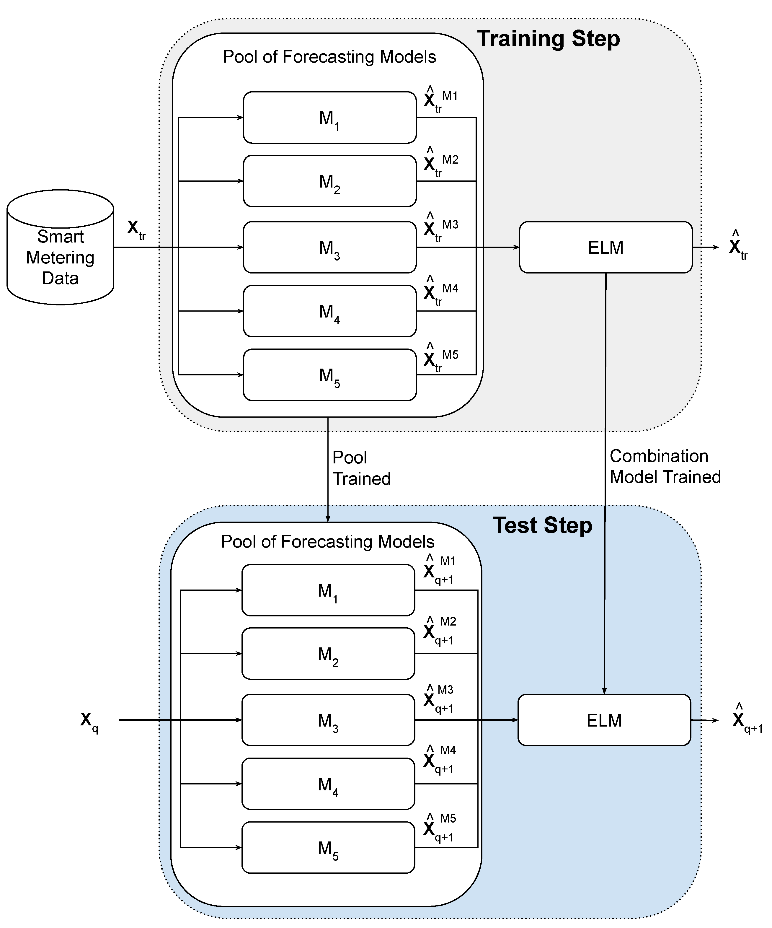
- The diversity of the ensemble is introduced by the employment of different forecasting methods such as autoregressive (AR), multilayer perceptron (MLP), extreme learning machine (ELM), radial basis function (RBF), and echo state network (ESN).
- The combination step employs an ELM model in order to map nonlinear relations between forecasts and to perform more accurate combinations.
- The proposed method is versatile, since different forecasting methods can be used in the pool, and then combined by the ELM.
2. Related Work
3. Proposed Ensemble Method
3.1. Single Model: Autoregressive Model
3.2. Single Model: Multilayer Perceptron (MLP)
3.3. Single Model: Echo State Networks (ESN)
3.4. Single Model: Radial Basis Function Network (RBF)
3.5. Single Model: Extreme Learning Machine (ELM)
4. Experimental Evaluation
4.1. Data Description
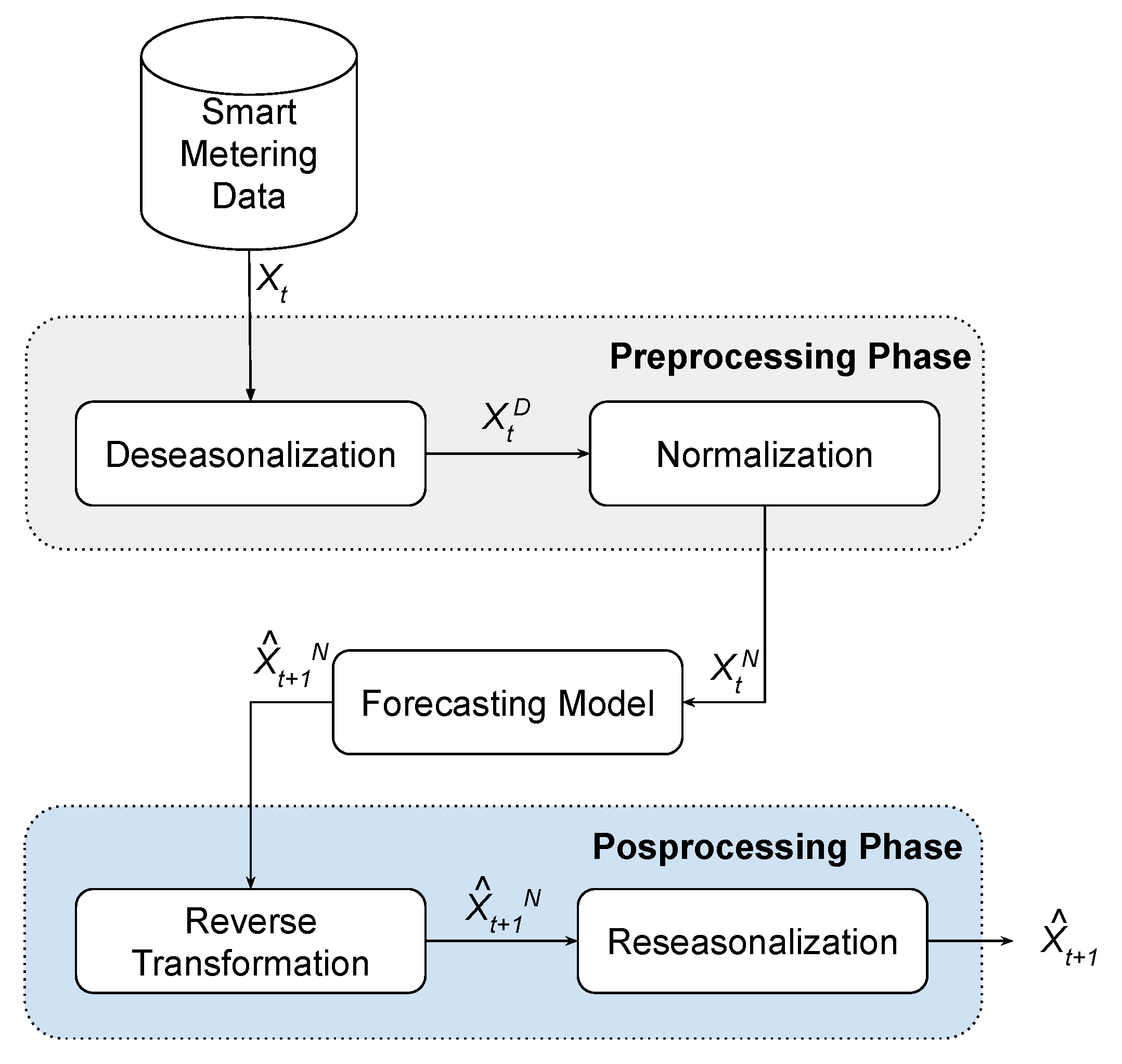
4.2. Preprocessing and Postprocessing Stages
4.3. Experimental Setup
- The coefficients of the AR model were calculated using the Yule–Walker equations, a closed-form solution [54];
- All artificial neural networks used hyperbolic tangent as activation function of the hidden neurons [59];
- The number of neurons in the hidden layer was determined by previous empirical tests, considering a range of [3:500].
- All models were implemented in Matlab®.
4.4. Error Metrics
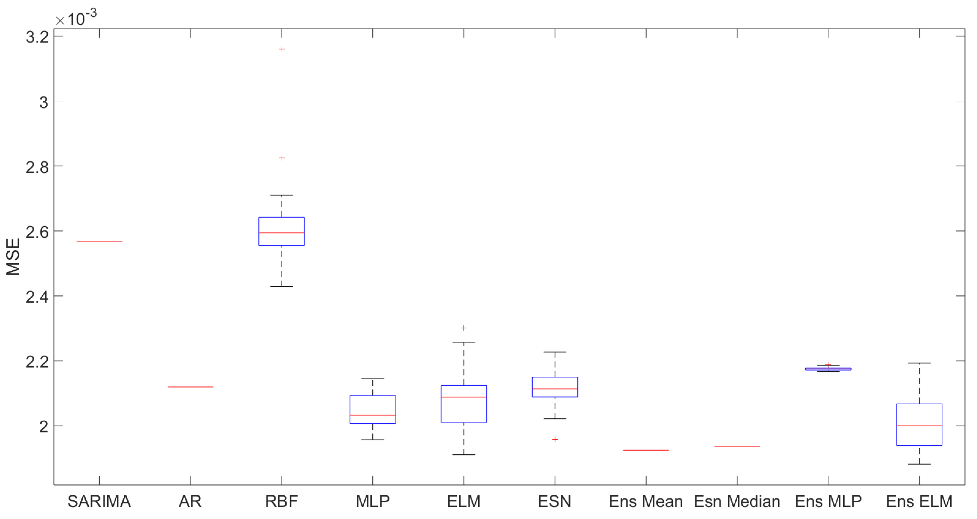
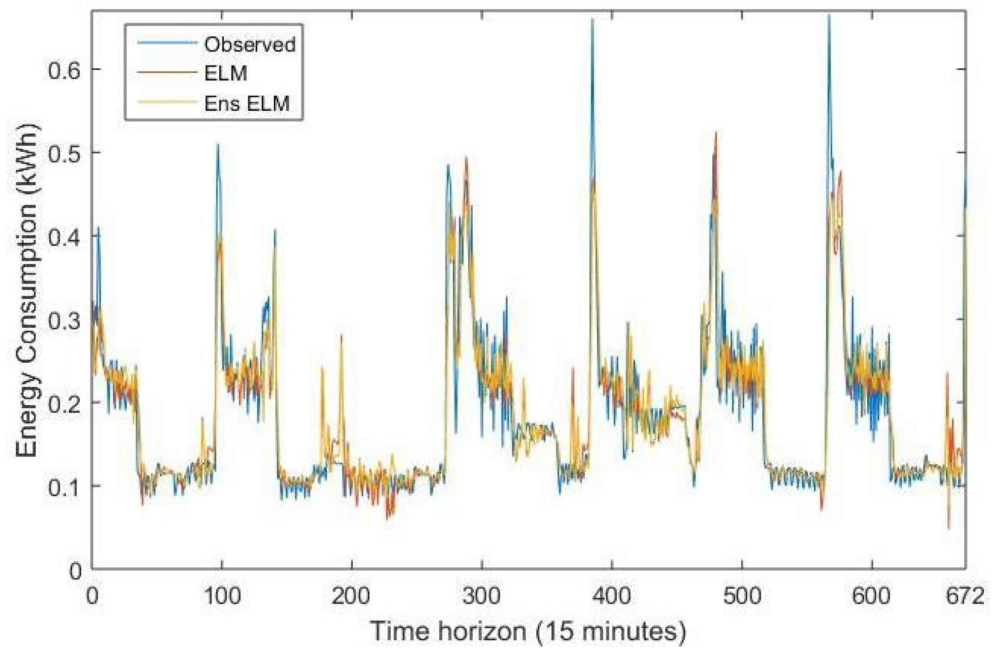
4.5. Results
4.6. Discussion
5. Conclusions
Author Contributions
Funding
Institutional Review Board Statement
Informed Consent Statement
Data Availability Statement
Acknowledgments
Conflicts of Interest
References
- Räsänen, T.; Voukantsis, D.; Niska, H.; Karatzas, K.; Kolehmainen, M. Data-based method for creating electricity use load profiles using large amount of customer-specific hourly measured electricity use data. Appl. Energy 2010, 87, 3538–3545. [Google Scholar] [CrossRef]
- Khan, Z.A.; Hussain, T.; Ullah, A.; Rho, S.; Lee, M.; Baik, S.W. Towards Efficient Electricity Forecasting in Residential and Commercial Buildings: A Novel Hybrid CNN with a LSTM-AE based Framework. Sensors 2020, 20, 1399. [Google Scholar] [CrossRef] [Green Version]
- Nejat, P.; Jomehzadeh, F.; Taheri, M.M.; Gohari, M.; Majid, M.Z.A. A global review of energy consumption, CO2 emissions and policy in the residential sector (with an overview of the top ten CO2 emitting countries). Renew. Sustain. Energy Rev. 2015, 43, 843–862. [Google Scholar] [CrossRef]
- Divina, F.; Gilson, A.; Goméz-Vela, F.; García Torres, M.; Torres, J.F. Stacking Ensemble Learning for Short-Term Electricity Consumption Forecasting. Energies 2018, 11, 949. [Google Scholar] [CrossRef] [Green Version]
- Kolokotsa, D. The role of smart grids in the building sector. Energy Build. 2016, 116, 703–708. [Google Scholar] [CrossRef] [Green Version]
- Hadri, S.; Najib, M.; Bakhouya, M.; Fakhri, Y.; El Arroussi, M. Performance Evaluation of Forecasting Strategies for Electricity Consumption in Buildings. Energies 2021, 14, 5831. [Google Scholar] [CrossRef]
- Lusis, P.; Khalilpour, K.R.; Andrew, L.; Liebman, A. Short-term residential load forecasting: Impact of calendar effects and forecast granularity. Appl. Energy 2017, 205, 654–669. [Google Scholar] [CrossRef]
- Alberg, D.; Last, M. Short-term load forecasting in smart meters with sliding window-based ARIMA algorithms. Vietnam. J. Comput. Sci. 2018, 5, 241–249. [Google Scholar] [CrossRef]
- Kumar Dubey, A.; Kumar, A.; García-Díaz, V.; Kumar Sharma, A.; Kanhaiya, K. Study and analysis of SARIMA and LSTM in forecasting time series data. Sustain. Energy Technol. Assessments 2021, 47, 101474. [Google Scholar] [CrossRef]
- Taskaya-Temizel, T.; Casey, M.C. A comparative study of autoregressive neural network hybrids. Neural Netw. 2005, 18, 781–789. [Google Scholar] [CrossRef] [Green Version]
- Kourentzes, N.; Barrow, D.; Petropoulos, F. Another look at forecast selection and combination: Evidence from forecast pooling. Int. J. Prod. Econ. 2019, 209, 226–235. [Google Scholar] [CrossRef] [Green Version]
- Cassales, G.; Gomes, H.; Bifet, A.; Pfahringer, B.; Senger, H. Improving the performance of bagging ensembles for data streams through mini-batching. Inf. Sci. 2021, 580, 260–282. [Google Scholar] [CrossRef]
- Kourentzes, N.; Barrow, D.K.; Crone, S.F. Neural network ensemble operators for time series forecasting. Expert Syst. Appl. 2014, 41, 4235–4244. [Google Scholar] [CrossRef] [Green Version]
- Huang, G.H.; Zhou, H.; Ding, X.; Zhang, R. Extreme learning machine for regression and multiclass classification. Trans. Syst. Man Cybern.—Part B Cybern. 2012, 42, 513–529. [Google Scholar] [CrossRef] [Green Version]
- Ahmad, T.; Chen, H. A review on machine learning forecasting growth trends and their real-time applications in different energy systems. Sustain. Cities Soc. 2020, 54, 102010. [Google Scholar] [CrossRef]
- Deb, C.; Zhang, F.; Yang, J.; Lee, S.E.; Shah, K.W. A review on time series forecasting techniques for building energy consumption. Renew. Sustain. Energy Rev. 2017, 74, 902–924. [Google Scholar] [CrossRef]
- Heydari, A.; Keynia, F.; Garcia, D.A.; De Santoli, L. Mid-Term Load Power Forecasting Considering Environment Emission using a Hybrid Intelligent Approach. In Proceedings of the 2018 5th International Symposium on Environment-Friendly Energies and Applications (EFEA), Rome, Italy, 24–26 September 2018; pp. 1–5. [Google Scholar]
- Chan, S.C.; Tsui, K.M.; Wu, H.C.; Hou, Y.; Wu, Y.; Wu, F.F. Load/Price Forecasting and Managing Demand Response for Smart Grids: Methodologies and Challenges. IEEE Signal Process. Mag. 2012, 29, 68–85. [Google Scholar] [CrossRef]
- Culaba, A.B.; Del Rosario, A.J.R.; Ubando, A.T.; Chang, J.S. Machine learning-based energy consumption clustering and forecasting for mixed-use buildings. Int. J. Energy Res. 2020, 44, 9659–9673. [Google Scholar] [CrossRef]
- Gao, Y.; Ruan, Y.; Fang, C.; Yin, S. Deep learning and transfer learning models of energy consumption forecasting for a building with poor information data. Energy Build. 2020, 223, 110156. [Google Scholar] [CrossRef]
- Pinto, T.; Praça, I.; Vale, Z.; Silva, J. Ensemble learning for electricity consumption forecasting in office buildings. Neurocomputing 2021, 423, 747–755. [Google Scholar] [CrossRef]
- Walther, J.; Weigold, M. A Systematic Review on Predicting and Forecasting the Electrical Energy Consumption in the Manufacturing Industry. Energies 2021, 14, 968. [Google Scholar] [CrossRef]
- Barzola-Monteses, J.; Espinoza-Andaluz, M.; Mite-León, M.; Flores-Morán, M. Energy Consumption of a Building by using Long Short-Term Memory Network: A Forecasting Study. In Proceedings of the 2020 39th IEEE International Conference of the Chilean Computer Science Society (SCCC), Coquimbo, Chile, 16–20 November 2020; pp. 1–6. [Google Scholar]
- Rana, M.; Koprinska, I. Forecasting electricity load with advanced wavelet neural networks. Neurocomputing 2016, 182, 118–132. [Google Scholar] [CrossRef]
- Zolfaghari, M.; Golabi, M.R. Modeling and predicting the electricity production in hydropower using conjunction of wavelet transform, long short-term memory and random forest models. Renew. Energy 2021, 170, 1367–1381. [Google Scholar] [CrossRef]
- El-Hendawi, M.; Wang, Z. An ensemble method of full wavelet packet transform and neural network for short term electrical load forecasting. Electr. Power Syst. Res. 2020, 182, 106265. [Google Scholar] [CrossRef]
- Gajowniczek, K.; Ząbkowski, T. Short term electricity forecasting using individual smart meter data. Procedia Comput. Sci. 2014, 35, 589–597. [Google Scholar] [CrossRef] [Green Version]
- Zhukov, A.V.; Sidorov, D.N.; Foley, A.M. Random forest based approach for concept drift handling. In International Conference on Analysis of Images, Social Networks and Texts; Springer: Berlin/Heidelberg, Germany, 2016; pp. 69–77. [Google Scholar]
- Heydari, A.; Nezhad, M.M.; Pirshayan, E.; Garcia, D.A.; Keynia, F.; De Santoli, L. Short-term electricity price and load forecasting in isolated power grids based on composite neural network and gravitational search optimization algorithm. Appl. Energy 2020, 277, 115503. [Google Scholar] [CrossRef]
- Heydari, A.; Garcia, D.A.; Keynia, F.; Bisegna, F.; Santoli, L.D. Hybrid intelligent strategy for multifactor influenced electrical energy consumption forecasting. Energy Sources Part B Econ. Plan. Policy 2019, 14, 341–358. [Google Scholar] [CrossRef]
- Yu, C.N.; Mirowski, P.; Ho, T.K. A sparse coding approach to household electricity demand forecasting in smart grids. IEEE Trans. Smart Grid 2016, 8, 738–748. [Google Scholar] [CrossRef]
- Fekri, M.N.; Patel, H.; Grolinger, K.; Sharma, V. Deep learning for load forecasting with smart meter data: Online Adaptive Recurrent Neural Network. Appl. Energy 2021, 282, 116177. [Google Scholar] [CrossRef]
- Li, L.; Meinrenken, C.J.; Modi, V.; Culligan, P.J. Short-term apartment-level load forecasting using a modified neural network with selected auto-regressive features. Appl. Energy 2021, 287, 116509. [Google Scholar] [CrossRef]
- Komatsu, H.; Kimura, O. Peak demand alert system based on electricity demand forecasting for smart meter data. Energy Build. 2020, 225, 110307. [Google Scholar] [CrossRef]
- Sajjad, M.; Khan, Z.A.; Ullah, A.; Hussain, T.; Ullah, W.; Lee, M.Y.; Baik, S.W. A novel CNN-GRU-based hybrid approach for short-term residential load forecasting. IEEE Access 2020, 8, 143759–143768. [Google Scholar] [CrossRef]
- Wang, Y.; Gan, D.; Sun, M.; Zhang, N.; Lu, Z.; Kang, C. Probabilistic individual load forecasting using pinball loss guided LSTM. Appl. Energy 2019, 235, 10–20. [Google Scholar] [CrossRef] [Green Version]
- Zhang, L.; Wen, J.; Li, Y.; Chen, J.; Ye, Y.; Fu, Y.; Livingood, W. A review of machine learning in building load prediction. Appl. Energy 2021, 285, 116452. [Google Scholar] [CrossRef]
- Somu, N.; Raman M R, G.; Ramamritham, K. A deep learning framework for building energy consumption forecast. Renew. Sustain. Energy Rev. 2021, 137, 110591. [Google Scholar] [CrossRef]
- Chou, J.S.; Truong, D.N. Multistep energy consumption forecasting by metaheuristic optimization of time-series analysis and machine learning. Int. J. Energy Res. 2021, 45, 4581–4612. [Google Scholar] [CrossRef]
- Chou, J.S.; Truong, D.N. A novel metaheuristic optimizer inspired by behavior of jellyfish in ocean. Appl. Math. Comput. 2021, 389, 125535. [Google Scholar] [CrossRef]
- Bouktif, S.; Fiaz, A.; Ouni, A.; Serhani, M. Multi-sequence LSTM-RNN deep learning and metaheuristics for electric load forecasting. Energies 2020, 13, 391. [Google Scholar] [CrossRef] [Green Version]
- Wichard, J.D.; Ogorzalek, M. Time series prediction with ensemble models. In Proceedings of the 2004 IEEE International Joint Conference on Neural Networks, Budapest, Hungary, 25–29 July 2004; Volume 2, pp. 1625–1630. [Google Scholar]
- de Mattos Neto, P.S.; Madeiro, F.; Ferreira, T.A.; Cavalcanti, G.D. Hybrid intelligent system for air quality forecasting using phase adjustment. Eng. Appl. Artif. Intell. 2014, 32, 185–191. [Google Scholar] [CrossRef]
- Firmino, P.R.A.; de Mattos Neto, P.S.; Ferreira, T.A. Correcting and combining time series forecasters. Neural Netw. 2014, 50, 1–11. [Google Scholar] [CrossRef]
- Belotti, J.; Siqueira, H.; Araujo, L.; Stevan, S.L.; de Mattos Neto, P.S.; Marinho, M.H.; de Oliveira, J.F.L.; Usberti, F.; Leone Filho, M.d.A.; Converti, A.; et al. Neural-Based Ensembles and Unorganized Machines to Predict Streamflow Series from Hydroelectric Plants. Energies 2020, 13, 4769. [Google Scholar] [CrossRef]
- de Mattos Neto, P.S.; de Oliveira, J.F.L.; Júnior, D.S.d.O.S.; Siqueira, H.V.; Marinho, M.H.D.N.; Madeiro, F. A Hybrid Nonlinear Combination System for Monthly Wind Speed Forecasting. IEEE Access 2020, 8, 191365–191377. [Google Scholar] [CrossRef]
- Siqueira, H.; Boccato, L.; Attux, R.; Lyra, C. Unorganized machines for seasonal streamflow series forecasting. Int. J. Neural Syst. 2014, 24, 1430009. [Google Scholar] [CrossRef] [PubMed]
- Domingos, S.d.O.; de Oliveira, J.F.; de Mattos Neto, P.S. An intelligent hybridization of ARIMA with machine learning models for time series forecasting. Knowl.-Based Syst. 2019, 175, 72–86. [Google Scholar]
- Siqueira, H.; Luna, I.; Alves, T.A.; de Souza Tadano, Y. The direct connection between box & Jenkins methodology and adaptive filtering theory. Math. Eng. Sci. Aerosp. (MESA) 2019, 10, 27–40. [Google Scholar]
- Yu, L.; Wang, S.; Lai, K.K. A novel nonlinear ensemble forecasting model incorporating GLAR and ANN for foreign exchange rates. Comput. Oper. Res. 2005, 32, 2523–2541. [Google Scholar] [CrossRef]
- Yang, D. Spatial prediction using kriging ensemble. Sol. Energy 2018, 171, 977–982. [Google Scholar] [CrossRef]
- Kim, D.; Hur, J. Short-term probabilistic forecasting of wind energy resources using the enhanced ensemble method. Energy 2018, 157, 211–226. [Google Scholar] [CrossRef]
- Berardi, V.; Zhang, G. An empirical investigation of bias and variance in time series forecasting: Modeling considerations and error evaluation. IEEE Trans. Neural Netw. 2003, 14, 668–679. [Google Scholar] [CrossRef]
- Box, G.E.; Jenkins, G.M.; Reinsel, G.C.; Ljung, G.M. Time Series Analysis: Forecasting and Control; John Wiley & Sons: Hoboken, NJ, USA, 2015. [Google Scholar]
- Zhang, G.P.; Qi, M. Neural network forecasting for seasonal and trend time series. Eur. J. Oper. Res. 2005, 160, 501–514. [Google Scholar] [CrossRef]
- Rendon-Sanchez, J.F.; de Menezes, L.M. Structural combination of seasonal exponential smoothing forecasts applied to load forecasting. Eur. J. Oper. Res. 2019, 275, 916–924. [Google Scholar] [CrossRef]
- Werbos, P.J. Beyond Regression: New Tools for Prediction and Analysis in the Behavioral Sciences. Ph.D. Thesis, Harvard University, Cambridge, UK, 1974. [Google Scholar]
- Rumelhart, D.E.; Hinton, G.E.; Williams, R.J. Learning representations by back-propagating errors. Cogn. Model. 1986, 5, 1. [Google Scholar] [CrossRef]
- Haykin, S.S. Neural Networks and Learning Machines/Simon Haykin; Prentice Hall: New York, NY, USA, 2009. [Google Scholar]
- Jaeger, H. The “echo state” approach to analysing and training recurrent neural networks-with an erratum note. Ger. Natl. Res. Cent. Inf. Technol. 2001, 148, 13. [Google Scholar]
- Siqueira, H.; Boccato, L.; Attux, R.; Lyra Filho, C. Echo state networks for seasonal streamflow series forecasting. In International Conference on Intelligent Data Engineering and Automated Learning; Springer: Berlin/Heidelberg, Germany, 2012; pp. 226–236. [Google Scholar]
- Siqueira, H.; Boccato, L.; Luna, I.; Attux, R.; Lyra, C. Performance analysis of unorganized machines in streamflow forecasting of brazilian plants. Appl. Soft Comput. 2018, 68, 494–506. [Google Scholar] [CrossRef]
- Siqueira, H.; Luna, I. Performance comparison of feedforward neural networks applied to stream flow series forecasting. Math. Eng. Sci. Aerosp. 2019, 10, 41–53. [Google Scholar]
- Chou, J.S.; Ngo, N.T. Time series analytics using sliding window metaheuristic optimization-based machine learning system for identifying building energy consumption patterns. Appl. Energy 2016, 177, 751–770. [Google Scholar] [CrossRef]
- de Mattos Neto, P.S.; Firmino, P.R.A.; Siqueira, H.; Tadano, Y.D.S.; Alves, T.A.; De Oliveira, J.F.L.; Marinho, M.H.D.N.; Madeiro, F. Neural-Based Ensembles for Particulate Matter Forecasting. IEEE Access 2021, 9, 14470–14490. [Google Scholar] [CrossRef]
- Hyndman, R.; Khandakar, Y. Automatic Time Series Forecasting: The forecast package for R. J. Stat. Software 2008, 27, 1–22. [Google Scholar] [CrossRef] [Green Version]
- Hyndman, R.J.; Koehler, A.B. Another look at measures of forecast accuracy. Int. J. Forecast. 2006, 22, 679–688. [Google Scholar] [CrossRef] [Green Version]
- Siqueira, H.; Macedo, M.; Tadano, Y.d.S.; Alves, T.A.; Stevan, S.L.; Oliveira, D.S.; Marinho, M.H.; Neto, P.S.; de Oliveira, J.F.; Luna, I.; et al. Selection of temporal lags for predicting riverflow series from hydroelectric plants using variable selection methods. Energies 2020, 13, 4236. [Google Scholar] [CrossRef]
- Diebold, F.X.; Mariano, R.S. Comparing predictive accuracy. J. Bus. Econ. Stat. 2002, 20, 134–144. [Google Scholar] [CrossRef]
- Harvey, D.; Leybourne, S.; Newbold, P. Testing the equality of prediction mean squared errors. Int. J. Forecast. 1997, 13, 281–291. [Google Scholar] [CrossRef]
- Brownlee, J. Statistical Methods for Machine Learning: Discover How to Transform Data into Knowledge with Python; Machine Learning Mastery: San Francisco, CA, USA, 2018. [Google Scholar]
- Demšar, J. Statistical comparisons of classifiers over multiple data sets. J. Mach. Learn. Res. 2006, 7, 1–30. [Google Scholar]


| Set | Number of Samples | Mean (kWh) | Standard Deviation |
|---|---|---|---|
| Whole Series | 2880 | 0.20077 | 0.10115 |
| Training | 1824 | 0.20794 | 0.10238 |
| Validation | 384 | 0.19789 | 0.10065 |
| Test | 672 | 0.18296 | 0.09579 |
| Model | Measure | Monday | Tuesday | Wednesday | Thursday | Friday | Saturday | Sunday | Max | Min | |
|---|---|---|---|---|---|---|---|---|---|---|---|
| Single | SARIMA | MSE ( kWh) | 2.8720 | 2.7614 | 3.3822 | 2.9381 | 1.7513 | 2.0152 | 2.2561 | 3.3822 | 1.7513 |
| MAE (kWh) | 0.0325 | 0.0332 | 0.0359 | 0.0353 | 0.0217 | 0.0288 | 0.0246 | 0.0359 | 0.0217 | ||
| MAPE (%) | 15.8363 | 14.2251 | 17.1321 | 19.2733 | 13.2665 | 16.0358 | 14.9922 | 19.2733 | 13.2665 | ||
| RMSE (kWh) | 0.0535 | 0.0525 | 0.0581 | 0.0542 | 0.0418 | 0.0448 | 0.0474 | 0.0581 | 0.0418 | ||
| IA | 0.8400 | 0.8991 | 0.9272 | 0.8162 | 0.8970 | 0.9296 | 0.9419 | 0.9419 | 0.8162 | ||
| AR | MSE ( kWh) | 1.1708 | 1.8802 | 1.9812 | 1.8478 | 2.2187 | 3.4516 | 2.2879 | 3.4516 | 1.1708 | |
| MAE (kWh) | 0.0225 | 0.0297 | 0.0234 | 0.0300 | 0.0281 | 0.0355 | 0.0337 | 0.0355 | 0.0225 | ||
| MAPE (%) | 14.3075 | 17.0181 | 14.9965 | 16.1628 | 11.8905 | 15.8668 | 19.7286 | 19.7286 | 11.8905 | ||
| RMSE (kWh) | 0.0342 | 0.0434 | 0.0445 | 0.0430 | 0.0471 | 0.0588 | 0.0478 | 0.0588 | 0.0342 | ||
| IA | 0.9355 | 0.9304 | 0.9568 | 0.9027 | 0.9202 | 0.9285 | 0.8827 | 0.9568 | 0.8827 | ||
| MLP | MSE ( kWh) | 1.1413 | 1.7036 | 1.8264 | 1.7168 | 2.1059 | 3.2103 | 1.9979 | 3.2103 | 1.1413 | |
| MAE (kWh) | 0.0217 | 0.0282 | 0.0216 | 0.0286 | 0.0289 | 0.0332 | 0.0304 | 0.0332 | 0.0216 | ||
| MAPE (%) | 13.5270 | 15.7165 | 12.6500 | 15.4307 | 12.3867 | 14.9471 | 17.9853 | 17.9853 | 12.3867 | ||
| RMSE (kWh) | 0.0338 | 0.0413 | 0.0427 | 0.0414 | 0.0459 | 0.0567 | 0.0447 | 0.0567 | 0.0338 | ||
| IA | 0.9367 | 0.9375 | 0.9583 | 0.9100 | 0.9260 | 0.9325 | 0.9000 | 0.9583 | 0.9000 | ||
| ELM | MSE ( kWh) | 1.1526 | 1.6701 | 1.7890 | 1.7343 | 2.0591 | 3.1423 | 1.8294 | 3.1423 | 1.1526 | |
| MAE (kWh) | 0.0209 | 0.0271 | 0.0222 | 0.0285 | 0.0292 | 0.0329 | 0.0287 | 0.0329 | 0.0209 | ||
| MAPE (%) | 12.7378 | 15.2818 | 13.9267 | 15.4566 | 12.6752 | 14.6467 | 17.0593 | 17.0593 | 12.6752 | ||
| RMSE (kWh) | 0.0340 | 0.0409 | 0.0423 | 0.0416 | 0.0454 | 0.0561 | 0.0428 | 0.0561 | 0.0340 | ||
| IA | 0.9356 | 0.9383 | 0.9594 | 0.9091 | 0.9284 | 0.9322 | 0.9079 | 0.9594 | 0.9079 | ||
| ESN | MSE ( kWh) | 1.1806 | 1.5424 | 1.7851 | 1.7948 | 1.9928 | 3.3204 | 2.0896 | 3.3204 | 1.1806 | |
| MAE (kWh) | 0.0213 | 0.0269 | 0.0220 | 0.0293 | 0.0279 | 0.0336 | 0.0305 | 0.0336 | 0.0213 | ||
| MAPE (%) | 12.9235 | 15.4666 | 13.9666 | 15.9643 | 11.9069 | 14.9907 | 18.2586 | 18.2586 | 11.9069 | ||
| RMSE (kWh) | 0.0344 | 0.0393 | 0.0423 | 0.0424 | 0.0446 | 0.0576 | 0.0457 | 0.0576 | 0.0344 | ||
| IA | 0.9345 | 0.9460 | 0.9605 | 0.9044 | 0.9320 | 0.9320 | 0.8964 | 0.9605 | 0.8964 | ||
| RBF | MSE ( kWh) | 1.7832 | 1.7691 | 3.0669 | 2.1245 | 2.2380 | 3.4564 | 2.5668 | 3.4564 | 1.7691 | |
| MAE (kWh) | 0.0261 | 0.0287 | 0.0326 | 0.0313 | 0.0313 | 0.0368 | 0.0322 | 0.0368 | 0.0261 | ||
| MAPE (%) | 15.2994 | 15.4352 | 22.0301 | 17.4932 | 13.7047 | 17.3610 | 20.1081 | 22.0301 | 13.7047 | ||
| RMSE (kWh) | 0.0422 | 0.0421 | 0.0554 | 0.0461 | 0.0473 | 0.0588 | 0.0507 | 0.0588 | 0.0421 | ||
| IA | 0.8957 | 0.9364 | 0.9243 | 0.8828 | 0.9245 | 0.9242 | 0.8633 | 0.9364 | 0.8633 | ||
| Ensemble | Ensemble Mean | MSE ( kWh) | 1.1632 | 1.6345 | 1.8150 | 1.7466 | 2.0379 | 3.1300 | 1.9460 | 3.1300 | 1.1632 |
| MAE (kWh) | 0.0216 | 0.0277 | 0.0220 | 0.0289 | 0.0282 | 0.0325 | 0.0300 | 0.0325 | 0.0216 | ||
| MAPE (%) | 13.0506 | 15.4767 | 13.5962 | 15.7273 | 12.1594 | 14.2690 | 17.7973 | 17.7973 | 12.1594 | ||
| RMSE (kWh) | 0.0341 | 0.0404 | 0.0426 | 0.0418 | 0.0451 | 0.0559 | 0.0441 | 0.0559 | 0.0341 | ||
| IA | 0.9342 | 0.9404 | 0.9583 | 0.9061 | 0.9289 | 0.9336 | 0.8992 | 0.9583 | 0.8992 | ||
| Ensemble Median | MSE ( kWh) | 1.1378 | 1.6290 | 1.8093 | 1.7949 | 2.0108 | 3.1865 | 1.9856 | 3.1865 | 1.1378 | |
| MAE (kWh) | 0.0215 | 0.0279 | 0.0214 | 0.0294 | 0.0281 | 0.0332 | 0.0303 | 0.0332 | 0.0214 | ||
| MAPE (%) | 13.2260 | 15.7893 | 13.1504 | 15.9486 | 12.1569 | 14.8732 | 17.9705 | 17.9705 | 12.1569 | ||
| RMSE (kWh) | 0.0337 | 0.0404 | 0.0425 | 0.0424 | 0.0448 | 0.0564 | 0.0446 | 0.0564 | 0.0337 | ||
| IA | 0.9365 | 0.9409 | 0.9593 | 0.9046 | 0.9291 | 0.9329 | 0.8992 | 0.9593 | 0.8992 | ||
| Ensemble MLP | MSE ( kWh) | 1.1588 | 1.5856 | 1.7507 | 1.7038 | 1.9816 | 3.0892 | 1.7540 | 3.0892 | 1.1588 | |
| MAE (kWh) | 0.0210 | 0.0266 | 0.0219 | 0.0278 | 0.0292 | 0.0319 | 0.0275 | 0.0319 | 0.0210 | ||
| MAPE (%) | 12.7435 | 14.9182 | 13.5774 | 15.2293 | 12.6736 | 14.1799 | 16.2368 | 16.2368 | 12.6736 | ||
| RMSE (kWh) | 0.0340 | 0.0398 | 0.0418 | 0.0413 | 0.0445 | 0.0556 | 0.0419 | 0.0556 | 0.0340 | ||
| IA | 0.9357 | 0.9428 | 0.9592 | 0.9095 | 0.9300 | 0.9328 | 0.9117 | 0.9592 | 0.9095 | ||
| Ensemble ELM | MSE ( kWh) | 1.2162 | 1.7898 | 1.5592 | 1.7071 | 1.9356 | 3.4034 | 1.5598 | 3.4034 | 1.2162 | |
| MAE (kWh) | 0.0217 | 0.0261 | 0.0203 | 0.0278 | 0.0303 | 0.0296 | 0.0243 | 0.0303 | 0.0203 | ||
| MAPE (%) | 12.5109 | 15.0994 | 12.1248 | 14.8702 | 13.2287 | 13.0881 | 13.8786 | 15.0994 | 12.1248 | ||
| RMSE (kWh) | 0.0349 | 0.0423 | 0.0395 | 0.0413 | 0.0440 | 0.0583 | 0.0395 | 0.0583 | 0.0349 | ||
| IA | 0.9321 | 0.9382 | 0.9624 | 0.9124 | 0.9300 | 0.9249 | 0.9263 | 0.9624 | 0.9124 |
| Model | NN | MSE ( kWh) | MAE (kWh) | MAPE (%) | RMSE (kWh) | IA | |
|---|---|---|---|---|---|---|---|
| Single | SARIMA | - | 2.5675 | 0.0303 | 15.4004 | 0.0506 | 0.9129 |
| AR | - | 2.1195 | 0.0290 | 15.7090 | 0.0460 | 0.9318 | |
| MLP | 200 | 1.9574 | 0.0275 | 14.5376 | 0.0442 | 0.9391 | |
| ELM | 120 | 1.9110 | 0.0271 | 14.5393 | 0.0437 | 0.9405 | |
| ESN | 40 | 1.9579 | 0.0274 | 14.7819 | 0.0442 | 0.9402 | |
| RBF | 60 | 2.4292 | 0.0310 | 17.1017 | 0.0493 | 0.9226 | |
| Ensemble | Ensemble Mean | - | 1.9247 | 0.0273 | 14.5826 | 0.0439 | 0.9373 |
| Ensemble Median | - | 1.9363 | 0.0274 | 14.7307 | 0.0440 | 0.9375 | |
| Ensemble MLP | 40 | 2.1671 | 0.0284 | 14.2228 | 0.0466 | 0.9358 | |
| Ensemble ELM | 60 | 1.8817 | 0.0257 | 13.5424 | 0.0434 | 0.9410 |
| Models | p-Value (Ensemble ELM) | p-Value (ELM) |
|---|---|---|
| Ensemble ELM | — | 0.0013 |
| ELM | 0.0013 | — |
| SARIMA | 1.21 | 1.21 |
| AR | 7.47 | 0.0045 |
| MLP | 0.0241 | 0.0323 |
| ESN | 1.72 | 0.0478 |
| RBF | 3.01 | 3.01 |
| Ensemble Mean | 1.91 | 3.35 |
| Ensemble Median | 2.05 | 3.35 |
| Ensemble MLP | 8.48 | 1.35 |
| Model | MSE (kWh) | MAE (kWh) | MAPE (%) | RMSE (kWh) | IA | Mean | Rank | |
|---|---|---|---|---|---|---|---|---|
| Single | SARIMA | 10 | 9 | 8 | 10 | 10 | 9.4 | 9 |
| AR | 7 | 8 | 9 | 7 | 8 | 7.6 | 8 | |
| MLP | 5 | 6 | 3 | 5 | 4 | 4.6 | 5 | |
| ELM | 2 | 2 | 4 | 2 | 2 | 2.4 | 2 | |
| ESN | 6 | 4 | 7 | 6 | 3 | 5.2 | 6 | |
| RBF | 9 | 10 | 10 | 9 | 9 | 9.4 | 9 | |
| Ensemble | Ensemble Mean | 3 | 3 | 5 | 3 | 6 | 4 | 3 |
| Ensemble Median | 4 | 5 | 6 | 4 | 5 | 4.8 | 4 | |
| Ensemble MLP | 8 | 7 | 2 | 8 | 7 | 6.4 | 7 | |
| Ensemble ELM | 1 | 1 | 1 | 1 | 1 | 1 | 1 |
Publisher’s Note: MDPI stays neutral with regard to jurisdictional claims in published maps and institutional affiliations. |
© 2021 by the authors. Licensee MDPI, Basel, Switzerland. This article is an open access article distributed under the terms and conditions of the Creative Commons Attribution (CC BY) license (https://creativecommons.org/licenses/by/4.0/).
Share and Cite
de Mattos Neto, P.S.G.; de Oliveira, J.F.L.; Bassetto, P.; Siqueira, H.V.; Barbosa, L.; Alves, E.P.; Marinho, M.H.N.; Rissi, G.F.; Li, F. Energy Consumption Forecasting for Smart Meters Using Extreme Learning Machine Ensemble. Sensors 2021, 21, 8096. https://doi.org/10.3390/s21238096
de Mattos Neto PSG, de Oliveira JFL, Bassetto P, Siqueira HV, Barbosa L, Alves EP, Marinho MHN, Rissi GF, Li F. Energy Consumption Forecasting for Smart Meters Using Extreme Learning Machine Ensemble. Sensors. 2021; 21(23):8096. https://doi.org/10.3390/s21238096
Chicago/Turabian Stylede Mattos Neto, Paulo S. G., João F. L. de Oliveira, Priscilla Bassetto, Hugo Valadares Siqueira, Luciano Barbosa, Emilly Pereira Alves, Manoel H. N. Marinho, Guilherme Ferretti Rissi, and Fu Li. 2021. "Energy Consumption Forecasting for Smart Meters Using Extreme Learning Machine Ensemble" Sensors 21, no. 23: 8096. https://doi.org/10.3390/s21238096