
A Survey of Deep Convolutional Neural Networks Applied for Prediction of Plant Leaf Diseases


 ,
,  , and
, and
Abstract
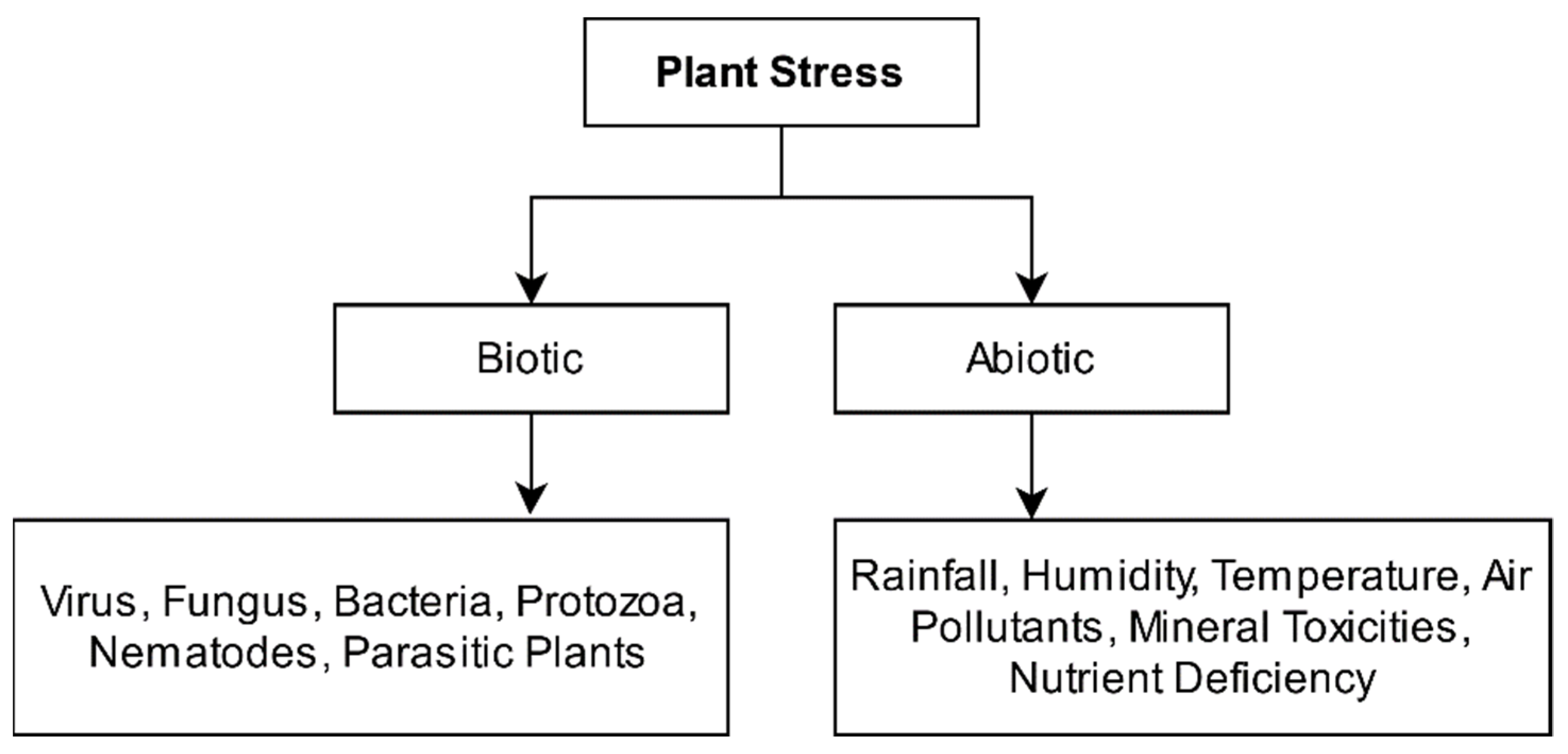
:1. Introduction
2. Materials and Methods
Recent Developments in Plant Leaf Disease Identification and Classification
3. Comparative Analysis
3.1. Pre-Processing Techniques
3.1.1. Resizing
3.1.2. Augmentation
3.1.3. Normalization and Standardization
3.1.4. Annotation
3.1.5. Outlier Rejection
3.1.6. Denoising
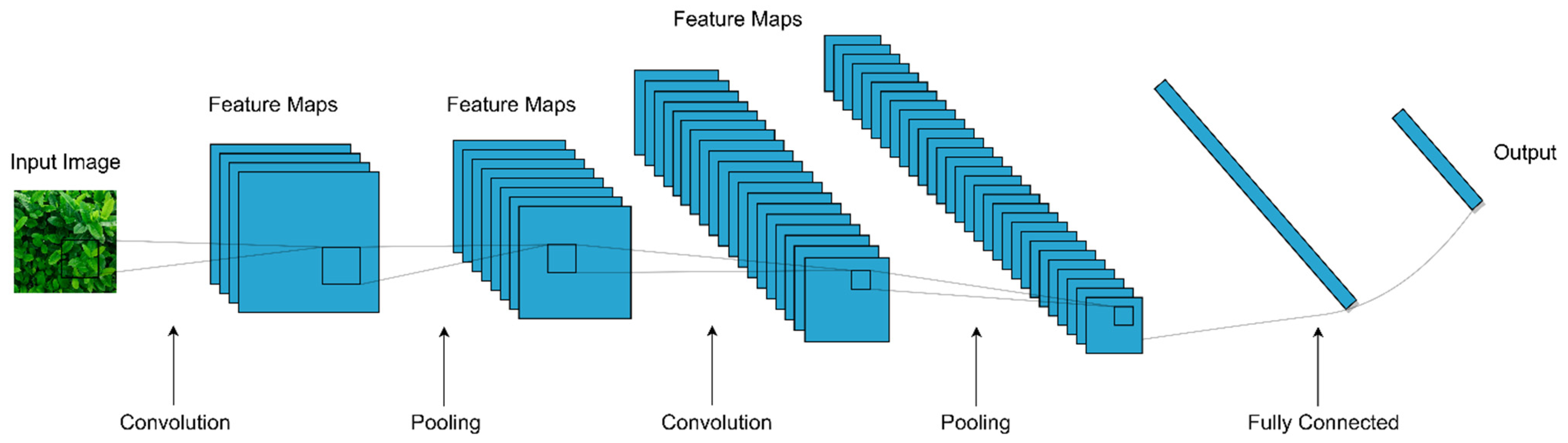
3.2. Convolutional Neural Networks
3.3. Datasets and CNN Models
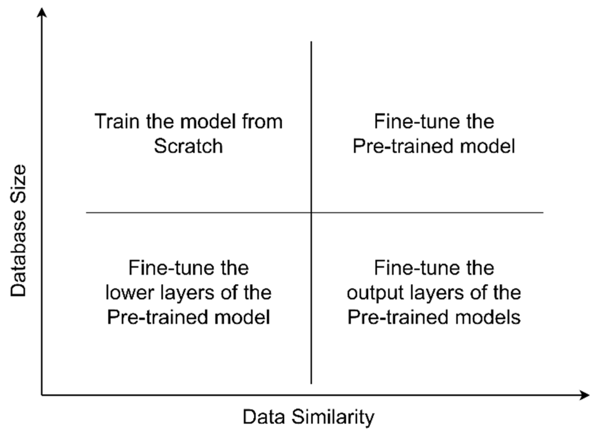
3.4. Common CNN Architectures
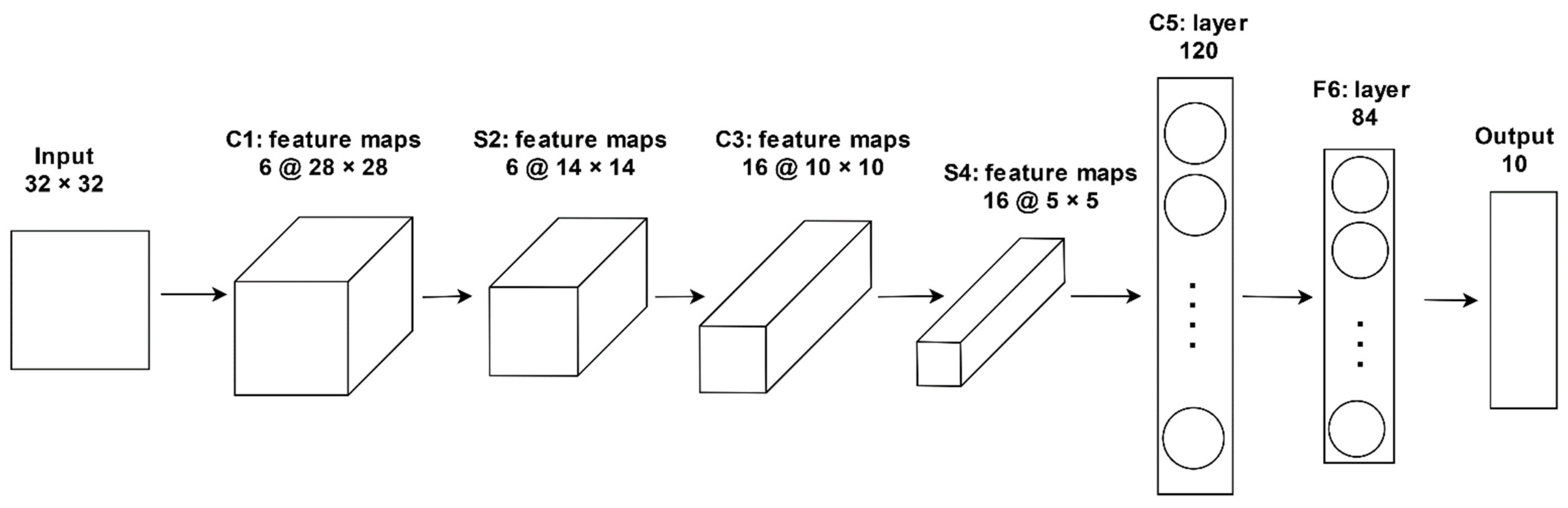
3.4.1. LeNet-5
3.4.2. AlexNet
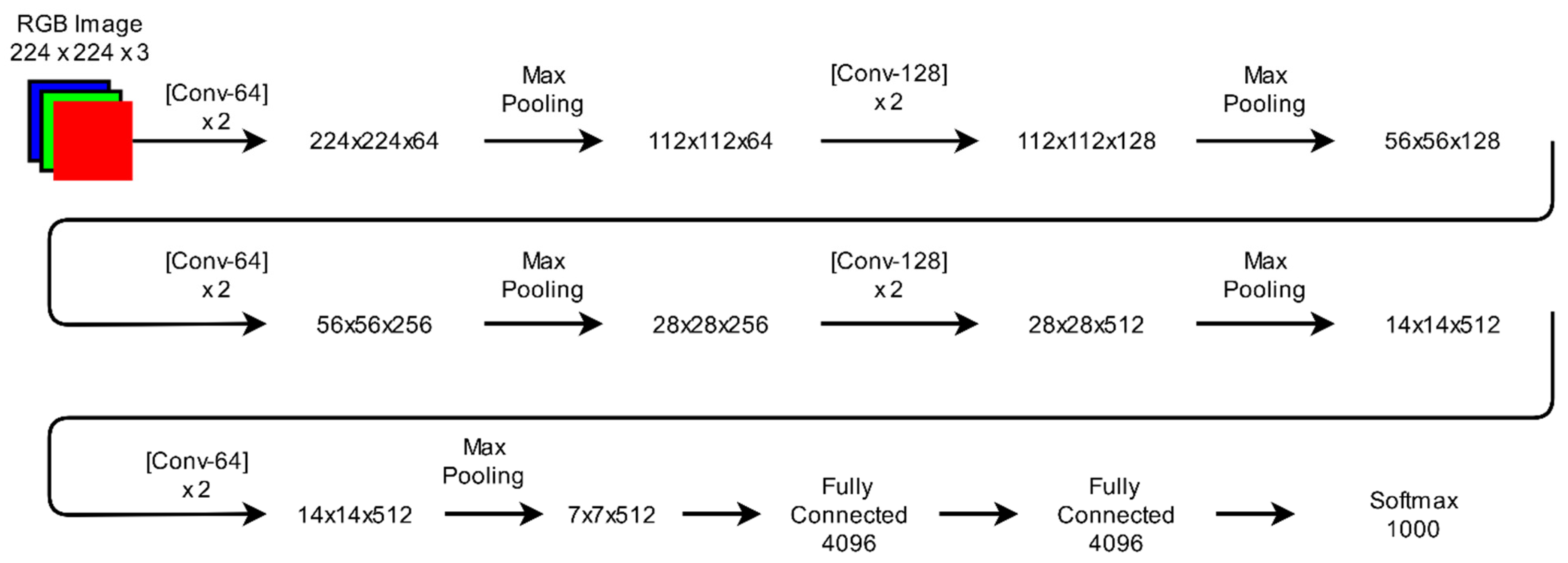
3.4.3. VGGNet
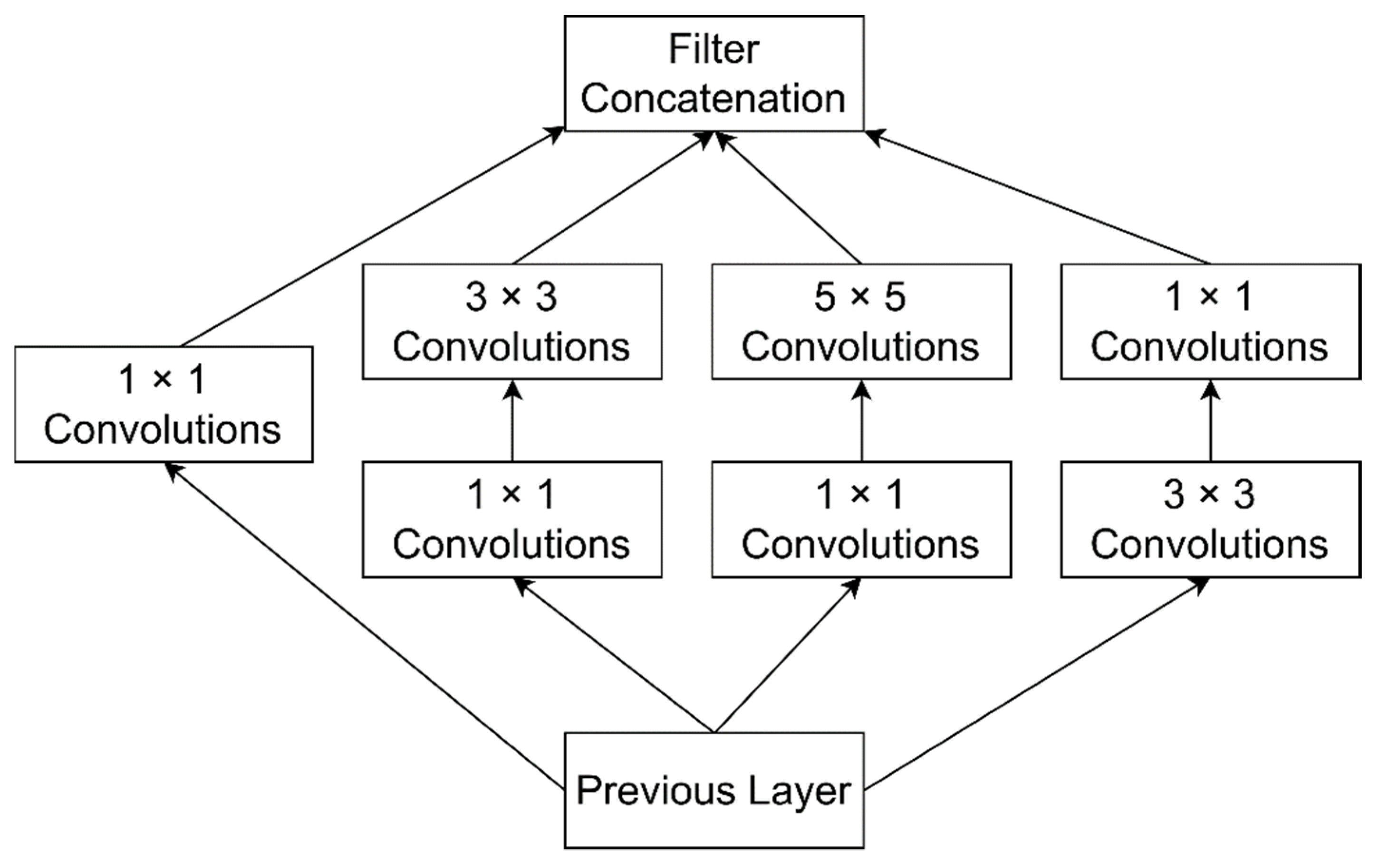
3.4.4. GoogLeNet
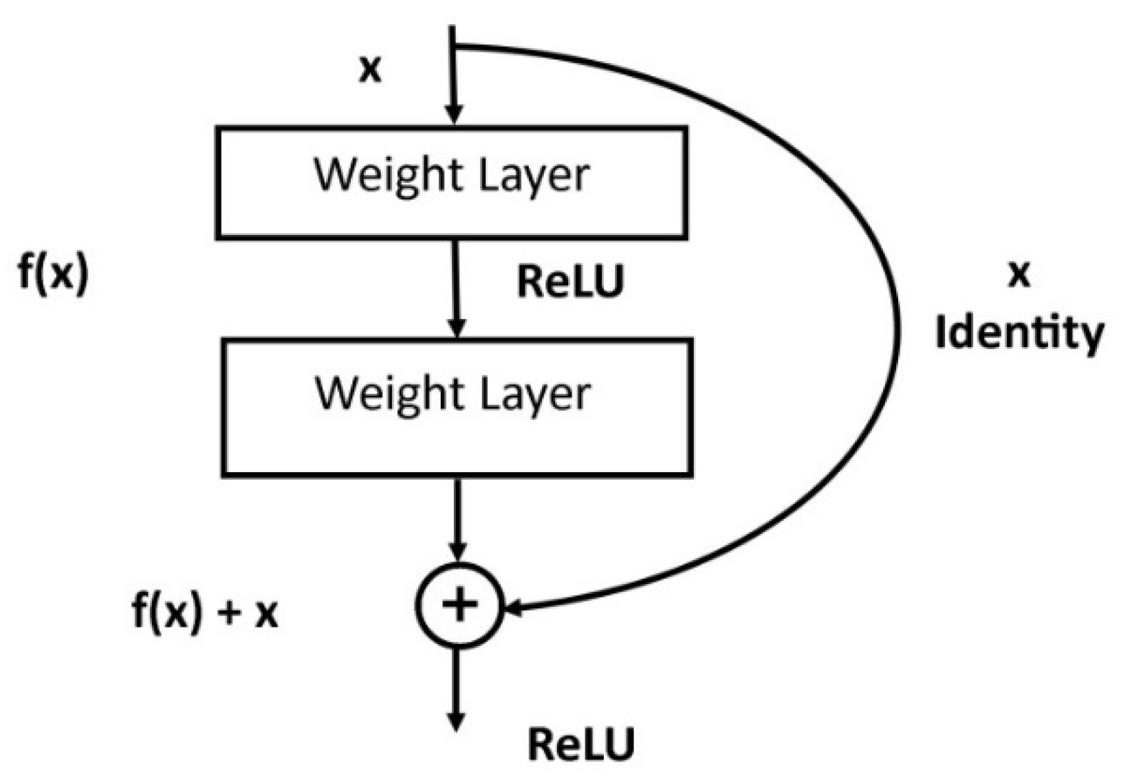
3.4.5. ResNet
3.4.6. ResNeXt
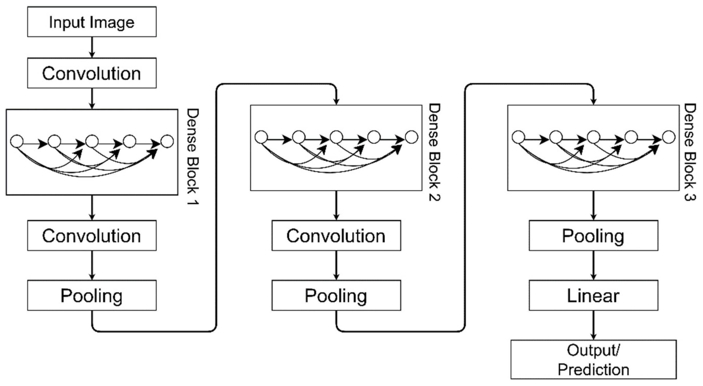
3.4.7. DenseNet
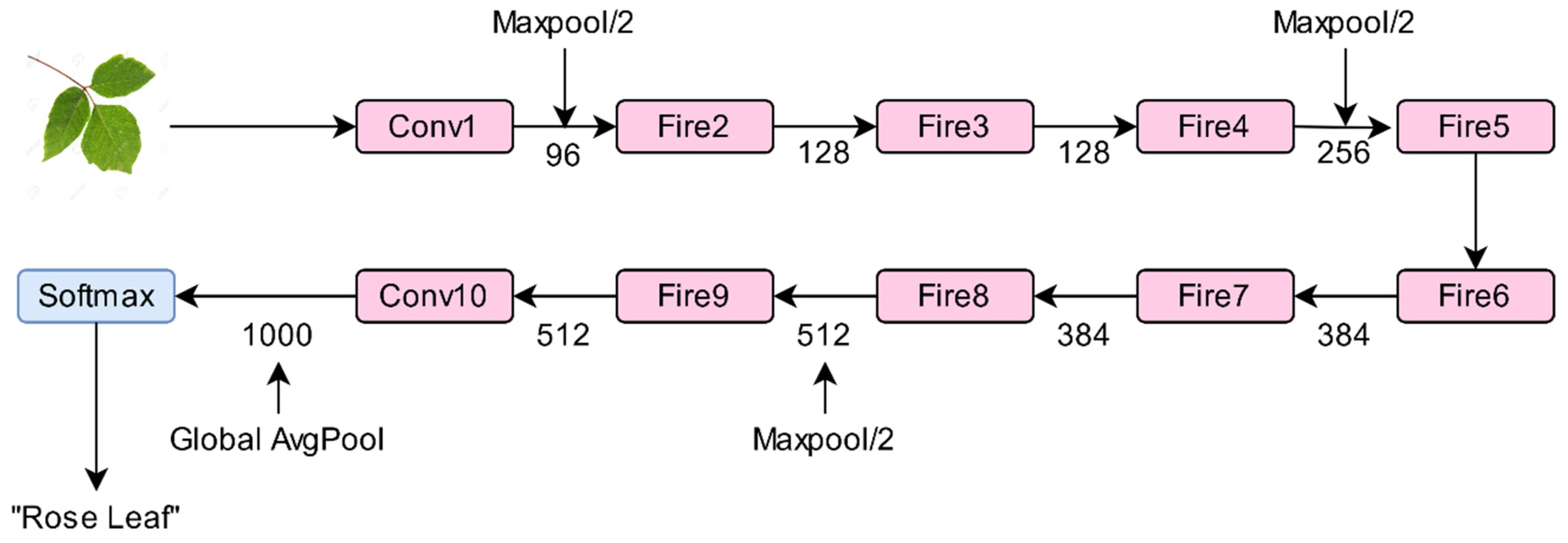
3.4.8. SqueezeNet
3.4.9. LeafNet
3.4.10. M-bCNN
3.4.11. Comparison of Common CNN Architectures
3.5. Optimization Techniques
3.5.1. Batch Gradient Descent (BGD) Optimization
3.5.2. Stochastic Gradient Descent (SGD) Algorithm
3.5.3. AdaGrad
3.5.4. Root Mean Square Propagation (RMSprop)
3.5.5. Adaptive Moment Estimation (Adam) Optimizer
3.6. Frameworks
3.6.1. TensorFlow
3.6.2. Theano
3.6.3. Keras
3.6.4. Caffe
3.6.5. Torch
3.6.6. Neuroph
3.6.7. Deeplearning4j
3.6.8. Pylearn2
3.6.9. DL MATLAB Toolbox
3.7. Analysis of DCNNs for Plant Leaf Disease Identification
4. Discussion and Conclusions
Author Contributions
Funding
Conflicts of Interest
References
- Zhang, W. A forecast analysis on world population and urbanization process. Environ. Dev. Sustain. 2008, 10, 717–730. [Google Scholar] [CrossRef]
- Chouhan, S.S.; Singh, U.P.; Jain, S. Applications of computer vision in plant pathology: A survey. Arch. Comput. Methods Eng. 2020, 27, 611–632. [Google Scholar] [CrossRef]
- Bock, C.H.; Poole, G.H.; Parker, P.E.; Gottwald, T.R. Plant disease severity estimated visually, by digital photography and image analysis, and by hyperspectral imaging. CRC Crit. Rev. Plant Sci. 2010, 29, 59–107. [Google Scholar] [CrossRef]
- Huang, K.-Y. Application of artificial neural network for detecting Phalaenopsis seedling diseases using color and texture features. Comput. Electron. Agric. 2007, 57, 3–11. [Google Scholar] [CrossRef]
- Huang, T.; Yang, R.; Huang, W.; Huang, Y.; Qiao, X. Detecting sugarcane borer diseases using support vector machine. Inf. Process. Agric. 2018, 5, 74–82. [Google Scholar] [CrossRef]
- Bauer, S.D.; Korč, F.; Förstner, W. The potential of automatic methods of classification to identify leaf diseases from multispectral images. Precis. Agric. 2011, 12, 361–377. [Google Scholar] [CrossRef]
- Li, Y.; Cao, Z.; Lu, H.; Xiao, Y.; Zhu, Y.; Cremers, A.B. In-field cotton detection via region-based semantic image segmentation. Comput. Electron. Agric. 2016, 127, 475–486. [Google Scholar] [CrossRef]
- Tan, W.; Zhao, C.; Wu, H. Intelligent alerting for fruit-melon lesion image based on momentum deep learning. Multimed. Tools Appl. 2016, 75, 16741–16761. [Google Scholar] [CrossRef]
- Pound, M.P.; Atkinson, J.A.; Townsend, A.J.; Wilson, M.H.; Griffiths, M.; Jackson, A.S.; Bulat, A.; Tzimiropoulos, G.; Wells, D.M.; Murchie, E.H.; et al. Deep machine learning provides state-of-the-art performance in image-based plant phenotyping. Gigascience 2017, 6, gix083. [Google Scholar] [CrossRef]
- Singh, A.; Ganapathysubramanian, B.; Singh, A.K.; Sarkar, S. Machine learning for high-throughput stress phenotyping in plants. Trends Plant Sci. 2016, 21, 110–124. [Google Scholar] [CrossRef] [Green Version]
- Ampatzidis, Y.; De Bellis, L.; Luvisi, A. iPathology: Robotic applications and management of plants and plant diseases. Sustainability 2017, 9, 1010. [Google Scholar] [CrossRef] [Green Version]
- Kaur, S.; Pandey, S.; Goel, S. Plants disease identification and classification through leaf images: A survey. Arch. Comput. Methods Eng. 2019, 26, 507–530. [Google Scholar] [CrossRef]
- Azimi, S.; Kaur, T.; Gandhi, T.K. A deep learning approach to measure stress level in plants due to Nitrogen deficiency. Measurement 2021, 173, 108650. [Google Scholar] [CrossRef]
- Noon, S.K.; Amjad, M.; Qureshi, M.A.; Mannan, A. Use of deep learning techniques for identification of plant leaf stresses: A review. Sustain. Comput. Inform. Syst. 2020, 28, 100443. [Google Scholar] [CrossRef]
- Barbedo, J.G.A. A review on the main challenges in automatic plant disease identification based on visible range images. Biosyst. Eng. 2016, 144, 52–60. [Google Scholar] [CrossRef]
- Chouhan, S.S.; Kaul, A.; Singh, U.P.; Jain, S. Bacterial foraging optimization based radial basis function neural network (BRBFNN) for identification and classification of plant leaf diseases: An automatic approach towards plant pathology. IEEE Access 2018, 6, 8852–8863. [Google Scholar] [CrossRef]
- Lu, Y.; Yi, S.; Zeng, N.; Liu, Y.; Zhang, Y. Identification of rice diseases using deep convolutional neural networks. Neurocomputing 2017, 267, 378–384. [Google Scholar] [CrossRef]
- Wang, G.; Sun, Y.; Wang, J. Automatic image-based plant disease severity estimation using deep learning. Comput. Intell. Neurosci. 2017, 2017, 2917536. [Google Scholar] [CrossRef] [Green Version]
- Ioffe, S.; Szegedy, C. Batch normalization: Accelerating deep network training by reducing internal covariate shift. In Proceedings of the International Conference on Machine Learning, Lille, France, 6–11 July 2015; pp. 448–456. [Google Scholar]
- Too, E.C.; Yujian, L.; Njuki, S.; Yingchun, L. A comparative study of fine-tuning deep learning models for plant disease identification. Comput. Electron. Agric. 2019, 161, 272–279. [Google Scholar] [CrossRef]
- Amara, J.; Bouaziz, B.; Algergawy, A. A deep learning-based approach for banana leaf diseases classification. In Datenbanksysteme für Business, Technology und Web (BTW 2017)-Workshopband; German Informatics Society: Bonn, Germany, 2017. [Google Scholar]
- Oppenheim, D.; Shani, G. Potato disease classification using convolution neural networks. Adv. Anim. Biosci. 2017, 8, 244. [Google Scholar] [CrossRef]
- Mohanty, S.P.; Hughes, D.P.; Salathé, M. Using deep learning for image-based plant disease detection. Front. Plant Sci. 2016, 7, 1–10. [Google Scholar] [CrossRef] [Green Version]
- Ferentinos, K.P. Deep learning models for plant disease detection and diagnosis. Comput. Electron. Agric. 2018, 145, 311–318. [Google Scholar] [CrossRef]
- Sladojevic, S.; Arsenovic, M.; Anderla, A.; Culibrk, D.; Stefanovic, D. Deep neural networks based recognition of plant diseases by leaf image classification. Comput. Intell. Neurosci. 2016, 2016, 3289801. [Google Scholar] [CrossRef] [Green Version]
- Ha, J.G.; Moon, H.; Kwak, J.T.; Hassan, S.I.; Dang, M.; Lee, O.N.; Park, H.Y. Deep convolutional neural network for classifying Fusarium wilt of radish from unmanned aerial vehicles. J. Appl. Remote Sens. 2017, 11, 1. [Google Scholar] [CrossRef]
- Khan, M.A.; Akram, T.; Sharif, M.; Awais, M.; Javed, K.; Ali, H.; Saba, T. CCDF: Automatic system for segmentation and recognition of fruit crops diseases based on correlation coefficient and deep CNN features. Comput. Electron. Agric. 2018, 155, 220–236. [Google Scholar] [CrossRef]
- Cruz, A.C.; Luvisi, A.; De Bellis, L.; Ampatzidis, Y. X-FIDO: An effective application for detecting olive quick decline syndrome with deep learning and data fusion. Front. Plant Sci. 2017, 8, 1–12. [Google Scholar] [CrossRef]
- Szegedy, C.; Vanhoucke, V.; Ioffe, S.; Shlens, J.; Wojna, Z. Rethinking the inception architecture for computer vision. Proc. IEEE Comput. Soc. Conf. Comput. Vis. Pattern Recognit. 2016, 2016, 2818–2826. [Google Scholar] [CrossRef] [Green Version]
- Chollet, F. Xception: Deep learning with depthwise separable convolutions. In Proceedings of the IEEE Conference on Computer Vision and Pattern Recognition, Honolulu, HI, USA, 21–26 July 2017; pp. 1251–1258. [Google Scholar]
- Simonyan, K.; Zisserman, A. Very deep convolutional networks for large-scale image recognition. In Proceedings of the 3rd International Conference on Learning Representations, San Diego, CA, USA, 7–9 May 2015; pp. 1–14. [Google Scholar]
- He, K.; Zhang, X.; Ren, S.; Sun, J. Deep residual learning for image recognition. In Proceedings of the IEEE Conference on Computer Vision and Pattern Recognition, Las Vegas, NV, USA, 27–30 July 2016; pp. 770–778. [Google Scholar]
- Huang, G.; Liu, Z.; Van Der Maaten, L.; Weinberger, K.Q. Densely connected convolutional networks. In Proceedings of the 30th IEEE Conference on Computer Vision and Pattern Recognition, Honolulu, HI, USA, 21–26 July 2017; Volume 2017, pp. 2261–2269. [Google Scholar]
- Boulent, J.; Foucher, S.; Théau, J.; St-Charles, P.-L. Convolutional neural networks for the automatic identification of plant diseases. Front. Plant Sci. 2019, 10, 941. [Google Scholar] [CrossRef] [Green Version]
- Brahimi, M.; Boukhalfa, K.; Moussaoui, A. Deep learning for tomato diseases: Classification and symptoms visualization. Appl. Artif. Intell. 2017, 31, 299–315. [Google Scholar] [CrossRef]
- Kawasaki, Y.; Uga, H.; Kagiwada, S.; Iyatomi, H. Basic study of automated diagnosis of viral plant diseases using convolutional neural networks. Int. Symp. Visual Comput. 2015, 9475, 842–850. [Google Scholar] [CrossRef]
- Ma, J.; Du, K.; Zheng, F.; Zhang, L.; Gong, Z.; Sun, Z. A recognition method for cucumber diseases using leaf symptom images based on deep convolutional neural network. Comput. Electron. Agric. 2018, 154, 18–24. [Google Scholar] [CrossRef]
- Lu, J.; Hu, J.; Zhao, G.; Mei, F.; Zhang, C. An in-field automatic wheat disease diagnosis system. Comput. Electron. Agric. 2017, 142, 369–379. [Google Scholar] [CrossRef] [Green Version]
- Liu, B.; Zhang, Y.; He, D.J.; Li, Y. Identification of apple leaf diseases based on deep convolutional neural networks. Symmetry 2018, 10, 11. [Google Scholar] [CrossRef] [Green Version]
- Durmuş, H.; Güneş, E.O.; Kırcı, M. Disease detection on the leaves of the tomato plants by using deep learning. In Proceedings of the 2017 6th International Conference on Agro-Geoinformatics, Fairfax, VA, USA, 7–10 August 2017; pp. 1–5. [Google Scholar]
- Ghosal, S.; Blystone, D.; Singh, A.K.; Ganapathysubramanian, B.; Singh, A.; Sarkar, S. An explainable deep machine vision framework for plant stress phenotyping. Proc. Natl. Acad. Sci. USA 2018, 115, 4613–4618. [Google Scholar] [CrossRef] [Green Version]
- Pawara, P.; Okafor, E.; Schomaker, L.; Wiering, M. Data augmentation for plant classification. In Proceedings of the International Conference on Advanced Concepts for Intelligent Vision Systems, Antwerp, Belgium, 18–21 September 2017; pp. 615–626. [Google Scholar]
- Barbedo, J.G.A. Factors influencing the use of deep learning for plant disease recognition. Biosyst. Eng. 2018, 172, 84–91. [Google Scholar] [CrossRef]
- Sa, I.; Ge, Z.; Dayoub, F.; Upcroft, B.; Perez, T.; McCool, C. DeepFruits: A fruit detection system using deep neural networks. Sensors 2016, 16, 1222. [Google Scholar] [CrossRef] [PubMed] [Green Version]
- Nguyen, T.T.-N.; Le, T.-L.; Vu, H.; Hoang, V.-S. Towards an automatic plant Identification system without dedicated dataset. Int. J. Mach. Learn. Comput. 2019, 9, 26–34. [Google Scholar] [CrossRef] [Green Version]
- Hubel, D.H.; Wiesel, T.N. Receptive fields, binocular interaction and functional architecture in the cat’s visual cortex. J. Physiol. 1962, 160, 106–154. [Google Scholar] [CrossRef]
- Traore, B.B.; Kamsu-Foguem, B.; Tangara, F. Deep convolution neural network for image recognition. Ecol. Inform. 2018, 48, 257–268. [Google Scholar] [CrossRef] [Green Version]
- LeCun, Y.; Boser, B.; Denker, J.S.; Henderson, D.; Howard, R.E.; Hubbard, W.; Jackel, L.D. Backpropagation applied to handwritten zip code recognition. Neural Comput. 1989, 1, 541–551. [Google Scholar] [CrossRef]
- Toda, Y.; Okura, F. How Convolutional neural networks diagnose plant disease. Plant Phenomics 2019, 2019, 9237136. [Google Scholar] [CrossRef] [PubMed]
- Singh, A.K.; Ganapathysubramanian, B.; Sarkar, S.; Singh, A. Deep learning for plant Stress phenotyping: Trends and future perspectives. Trends Plant Sci. 2018, 23, 883–898. [Google Scholar] [CrossRef] [Green Version]
- Mohanty, S. PlantVillage-Dataset. Available online: https://github.com/spMohanty/PlantVillage-Dataset (accessed on 30 June 2021).
- Ngugi, L.C.; Abelwahab, M.; Abo-Zahhad, M. Recent advances in image processing techniques for automated leaf pest and disease recognition—A review. Inf. Process. Agric. 2021, 8, 27–51. [Google Scholar] [CrossRef]
- Kundu, N.; Rani, G.; Dhaka, V.S. A Comparative analysis of deep learning models applied for disease classification in Bell pepper. In Proceedings of the 2020 Sixth International Conference on Parallel, Distributed and Grid Computing (PDGC), Solan, India, 6–8 November 2020; pp. 243–247. [Google Scholar]
- Liu, J.; Wang, X. Plant diseases and pests detection based on deep learning: A review. Plant Methods 2021, 17, 22. [Google Scholar] [CrossRef] [PubMed]
- Yadav, S.; Sengar, N.; Singh, A.; Singh, A.; Dutta, M.K. Identification of disease using deep learning and evaluation of bacteriosis in peach leaf. Ecol. Inform. 2021, 61, 101247. [Google Scholar] [CrossRef]
- N, K.; Narasimha Prasad, L.V.; Pavan Kumar, C.S.; Subedi, B.; Abraha, H.B.; V E, S. Rice leaf diseases prediction using deep neural networks with transfer learning. Environ. Res. 2021, 198, 111275. [Google Scholar] [CrossRef] [PubMed]
- Chen, J.; Zhang, D.; Zeb, A.; Nanehkaran, Y.A. Identification of rice plant diseases using lightweight attention networks. Expert Syst. Appl. 2021, 169, 114514. [Google Scholar] [CrossRef]
- Joshi, R.C.; Kaushik, M.; Dutta, M.K.; Srivastava, A.; Choudhary, N. VirLeafNet: Automatic analysis and viral disease diagnosis using deep-learning in Vigna mungo plant. Ecol. Inform. 2021, 61, 101197. [Google Scholar] [CrossRef]
- Bhatt, P.; Sarangi, S.; Pappula, S. Comparison of CNN models for application in crop health assessment with participatory sensing. In Proceedings of the 2017 IEEE Global Humanitarian Technology Conference (GHTC), San Jose, CA, USA, 19–22 October 2017. [Google Scholar] [CrossRef]
- Zhang, K.; Wu, Q.; Liu, A.; Meng, X. Can deep learning identify tomato leaf disease? Adv. Multimed. 2018, 2018, 6710865. [Google Scholar] [CrossRef] [Green Version]
- Sibiya, M.; Sumbwanyambe, M. A Computational procedure for the recognition and classification of maize leaf diseases out of healthy leaves using convolutional neural networks. AgriEngineering 2019, 1, 119–131. [Google Scholar] [CrossRef] [Green Version]
- Joly, A.; Goëau, H.; Glotin, H.; Spampinato, C.; Bonnet, P.; Vellinga, W.-P.; Lombardo, J.-C.; Planqué, R.; Palazzo, S.; Müller, H. Lifeclef 2017 lab overview: Multimedia species identification challenges. In Proceedings of the International Conference of the Cross-Language Evaluation Forum for European Languages, Dublin, Ireland, 11–14 September 2017; pp. 255–274. [Google Scholar]
- Mehdipour Ghazi, M.; Yanikoglu, B.; Aptoula, E. Plant identification using deep neural networks via optimization of transfer learning parameters. Neurocomputing 2017, 235, 228–235. [Google Scholar] [CrossRef]
- DeChant, C.; Wiesner-Hanks, T.; Chen, S.; Stewart, E.L.; Yosinski, J.; Gore, M.A.; Nelson, R.J.; Lipson, H. Automated identification of northern leaf blight-infected maize plants from field imagery using deep learning. Phytopathology 2017, 107, 1426–1432. [Google Scholar] [CrossRef] [PubMed] [Green Version]
- Arnal Barbedo, J.G. Plant disease identification from individual lesions and spots using deep learning. Biosyst. Eng. 2019, 180, 96–107. [Google Scholar] [CrossRef]
- Deng, J.; Dong, W.; Socher, R.; Li, L.-J.; Li, K.; Fei-Fei, L. Imagenet: A large-scale hierarchical image database. In Proceedings of the 2009 IEEE Conference on Computer Vision and Pattern Recognition, Miami, FL, USA, 20–25 June 2009; pp. 248–255. [Google Scholar]
- Everingham, M.; Van Gool, L.; Williams, C.K.I.; Winn, J.; Zisserman, A. The pascal visual object classes (VOC) challenge. Int. J. Comput. Vis. 2010, 88, 303–338. [Google Scholar] [CrossRef] [Green Version]
- Picon, A.; Alvarez-Gila, A.; Seitz, M.; Ortiz-Barredo, A.; Echazarra, J.; Johannes, A. Deep convolutional neural networks for mobile capture device-based crop disease classification in the wild. Comput. Electron. Agric. 2019, 161, 280–290. [Google Scholar] [CrossRef]
- Pan, S.J.; Yang, Q. A survey on transfer learning. IEEE Trans. Knowl. Data Eng. 2010, 22, 1345–1359. [Google Scholar] [CrossRef]
- Li, P. Optimization Algorithms for Deep Learning. 2017. Available online: http://lipiji.com/docs/li2017optdl.pdf (accessed on 30 June 2021).
- Mishkin, D.; Matas, J. All you need is a good init. In Proceedings of the International Conference on Learning Representations 2015, San Diego, CA, USA, 7–9 May 2015. [Google Scholar]
- Yu, D.; Xiong, W.; Droppo, J.; Stolcke, A.; Ye, G.; Li, J.; Zweig, G. Deep convolutional neural networks with layer-wise context expansion and attention. In Proceedings of the Interspeech 2016, San Francisco, CA, USA, 8–12 September 2016; pp. 17–21. [Google Scholar]
- LeCun, Y.; Bottou, L.; Bengio, Y.; Haffner, P. Gradient-based learning applied to document recognition. Proc. IEEE 1998. [Google Scholar] [CrossRef] [Green Version]
- Krizhevsky, A.; Sutskever, I.; Hinton, G.E. Imagenet classification with deep convolutional neural networks. In Proceedings of the 25th International Conference on Neural Information Processing Systems—Volume 1; Curran Associates Inc.: New York, NY, USA, 2012; pp. 1097–1105. [Google Scholar]
- Canziani, A.; Paszke, A.; Culurciello, E. An analysis of deep neural network models for practical applications. arXiv 2016, arXiv:1605.07678. [Google Scholar]
- Ding, W.; Taylor, G. Automatic moth detection from trap images for pest management. Comput. Electron. Agric. 2016, 123, 17–28. [Google Scholar] [CrossRef] [Green Version]
- Kerkech, M.; Hafiane, A.; Canals, R. Deep leaning approach with colorimetric spaces and vegetation indices for vine diseases detection in UAV images. Comput. Electron. Agric. 2018, 155, 237–243. [Google Scholar] [CrossRef]
- Szegedy, C.; Liu, W.; Jia, Y.; Sermanet, P.; Reed, S.; Anguelov, D.; Erhan, D.; Vanhoucke, V.; Rabinovich, A. Going deeper with convolutions. Proc. IEEE Comput. Soc. Conf. Comput. Vis. Pattern Recognit. 2015, 91, 2322–2330. [Google Scholar] [CrossRef] [Green Version]
- Lin, M.; Chen, Q.; Yan, S. Network in network. arXiv 2014, arXiv:1312.4400. [Google Scholar]
- Zagoruyko, S.; Komodakis, N. Wide residual networks. arXiv 2017, arXiv:1605.07146. [Google Scholar]
- Xie, S.; Girshick, R.; Dollár, P.; Tu, Z.; He, K. Aggregated residual transformations for deep neural networks. In Proceedings of the 2017 IEEE Conference on Computer Vision and Pattern Recognition, Honolulu, HI, USA, 21–26 July 2017; pp. 5987–5995. [Google Scholar] [CrossRef] [Green Version]
- Fuentes, A.; Yoon, S.; Kim, S.; Park, D. A Robust deep-learning-based detector for real-time tomato plant diseases and pests recognition. Sensors 2017, 17, 2022. [Google Scholar] [CrossRef] [Green Version]
- Iandola, F.N.; Han, S.; Moskewicz, M.W.; Ashraf, K.; Dally, W.J.; Keutzer, K. SqueezeNet: AlexNet-level accuracy with 50x fewer parameters and <0.5 MB model size. arXiv 2016, arXiv:1602.07360. [Google Scholar]
- Chen, J.; Liu, Q.; Gao, L. Visual tea leaf disease recognition using a convolutional neural network model. Symmetry 2019, 11, 343. [Google Scholar] [CrossRef] [Green Version]
- Lin, Z.; Mu, S.; Huang, F.; Mateen, K.A.; Wang, M.; Gao, W.; Jia, J. A unified matrix-based convolutional neural network for fine-grained image classification of wheat leaf diseases. IEEE Access 2019, 7, 11570–11590. [Google Scholar] [CrossRef]
- Liang, W.J.; Zhang, H.; Zhang, G.F.; Cao, H. Rice blast disease recognition using a deep convolutional neural network. Sci. Rep. 2019, 9, 2869. [Google Scholar] [CrossRef] [Green Version]
- Liu, L.; Ouyang, W.; Wang, X.; Fieguth, P.; Chen, J.; Liu, X.; Pietikäinen, M. Deep learning for generic Object detection: A survey. Int. J. Comput. Vis. 2020, 128, 261–318. [Google Scholar] [CrossRef] [Green Version]
- Li, H.; Lin, Z.; Shen, X.; Brandt, J.; Hua, G. A convolutional neural network cascade for face detection. In Proceedings of the IEEE Conference on Computer Vision and Pattern Recognition (CVPR), Boston, MA, USA, 7–12 June 2015. [Google Scholar]
- Adjabi, I.; Ouahabi, A.; Benzaoui, A.; Jacques, S. Multi-block color-binarized statistical images for single-sample face recognition. Sensors 2021, 21, 728. [Google Scholar] [CrossRef]
- Adjabi, I.; Ouahabi, A.; Benzaoui, A.; Taleb-ahmed, A. Past, Present, and future of face recognition: A review. Electronics 2020, 9, 1188. [Google Scholar] [CrossRef]
- Pradhan, N.; Dhaka, V.S.; Chaudhary, H. Classification of human bones using deep convolutional neural network. IOP Conf. Ser. Mater. Sci. Eng. 2019, 594, 12024. [Google Scholar] [CrossRef]
- Nair, P.P.; James, A.; Saravanan, C. Malayalam handwritten character recognition using convolutional neural network. In Proceedings of the 2017 International Conference on Inventive Communication and Computational Technologies (ICICCT), Coimbatore, India, 10–11 March 2017; pp. 278–281. [Google Scholar]
- Shustanov, A.; Yakimov, P. CNN Design for real-time traffic sign recognition. Procedia Eng. 2017, 201, 718–725. [Google Scholar] [CrossRef]
- Kuwata, K.; Shibasaki, R. Estimating crop yields with deep learning and remotely sensed data. In Proceedings of the 2015 IEEE International Geoscience and Remote Sensing Symposium (IGARSS), Milan, Italy, 26–31 July 2015; pp. 858–861. [Google Scholar]
- Xu, R.; Li, C.; Paterson, A.H.; Jiang, Y.; Sun, S.; Robertson, J.S. Aerial images and convolutional neural network for cotton bloom detection. Front. Plant Sci. 2018, 8, 2235. [Google Scholar] [CrossRef] [Green Version]
- Dyrmann, M.; Karstoft, H.; Midtiby, H.S. Plant species classification using deep convolutional neural network. Biosyst. Eng. 2016, 151, 72–80. [Google Scholar] [CrossRef]
- Han, S.; Mao, H.; Dally, W.J. Deep compression: Compressing deep neural networks with pruning, trained quantization and huffman coding. arXiv 2015, arXiv:1510.00149. [Google Scholar]
- Chen, S.W.; Shivakumar, S.S.; Dcunha, S.; Das, J.; Okon, E.; Qu, C.; Taylor, C.J.; Kumar, V. Counting apples and oranges with deep learning: A data-driven approach. IEEE Robot. Autom. Lett. 2017, 2, 781–788. [Google Scholar] [CrossRef]
- Pethybridge, S.J.; Nelson, S.C. Leaf doctor: A new portable application for quantifying plant disease severity. Plant Dis. 2015, 99, 1310–1316. [Google Scholar] [CrossRef] [PubMed] [Green Version]
- Tran, T.-T.; Choi, J.-W.; Le, T.-T.H.; Kim, J.-W. A Comparative study of deep CNN in forecasting and classifying the macronutrient deficiencies on development of tomato plant. Appl. Sci. 2019, 9, 1601. [Google Scholar] [CrossRef] [Green Version]
- Shakoor, N.; Lee, S.; Mockler, T.C. High throughput phenotyping to accelerate crop breeding and monitoring of diseases in the field. Curr. Opin. Plant Biol. 2017, 38, 184–192. [Google Scholar] [CrossRef]
- Dang, L.M.; Syed, I.H.; Suhyeon, I. Drone agriculture imagery system for radish wilt. J. Appl. Remote Sens. 2017, 11, 16006. [Google Scholar]
- Selvaraj, M.G.; Vergara, A.; Ruiz, H.; Safari, N.; Elayabalan, S.; Ocimati, W.; Blomme, G. AI-powered banana diseases and pest detection. Plant Methods 2019, 15, 1–11. [Google Scholar] [CrossRef]
- Ramcharan, A.; Baranowski, K.; McCloskey, P.; Ahmed, B.; Legg, J.; Hughes, D.P. Deep learning for image-based cassava disease detection. Front. Plant Sci. 2017, 8, 1–7. [Google Scholar] [CrossRef] [PubMed] [Green Version]
- Zhang, X.; Qiao, Y.; Meng, F.; Fan, C.; Zhang, M. Identification of maize leaf diseases using improved deep convolutional neural networks. IEEE Access 2018, 6, 30370–30377. [Google Scholar] [CrossRef]
- Nachtigall, L.G.; Araujo, R.M.; Nachtigall, G.R. Classification of apple tree disorders using convolutional neural networks. In Proceedings of the 2016 IEEE 28th International Conference on Tools with Artificial Intelligence (ICTAI), San Jose, CA, USA, 6–8 November 2016; pp. 472–476. [Google Scholar]
- Johannes, A.; Picon, A.; Alvarez-Gila, A.; Echazarra, J.; Rodriguez-Vaamonde, S.; Navajas, A.D.; Ortiz-Barredo, A. Automatic plant disease diagnosis using mobile capture devices, applied on a wheat use case. Comput. Electron. Agric. 2017, 138, 200–209. [Google Scholar] [CrossRef]
- Szegedy, C.; Ioffe, S.; Vanhoucke, V.; Alemi, A.A. Inception-v4, inception-resnet and the impact of residual connections on learning. Proc. Thirty-First AAAI Conf. Artif. Intell. 2017, 4278–4284. [Google Scholar] [CrossRef]
- Kingma, D.P.; Ba, J. Adam: A method for stochastic optimization. arXiv 2014, arXiv:1412.6980. [Google Scholar]
- Abadi, M.; Barham, P.; Chen, J.; Chen, Z.; Davis, A.; Dean, J.; Devin, M.; Ghemawat, S.; Irving, G.; Isard, M.; et al. TensorFlow: A system for large-scale machine learning. In Proceedings of the 12th Symposium on Operating Systems Design and Implementation, Savannah, GA, USA, 2–4 November 2016; pp. 265–283. [Google Scholar]
- Bastien, F.; Lamblin, P.; Pascanu, R.; Bergstra, J.; Goodfellow, I.; Bergeron, A.; Bouchard, N.; Warde-Farley, D.; Bengio, Y. Theano: New features and speed improvements. arXiv 2012, arXiv:1211.5590. [Google Scholar]
- Bergstra, J.; Breuleux, O.; Bastien, F.; Lamblin, P.; Pascanu, R.; Desjardins, G.; Turian, J.; Warde-Farley, D.; Bengio, Y. Theano: A CPU and GPU math compiler in Python. In Proceedings of the 9th Python in Science Conference, Austin, TX, USA, 28 June–3 July 2010; Volume 1, pp. 3–10. [Google Scholar]
- Team, T.T.D.; Al-Rfou, R.; Alain, G.; Almahairi, A.; Angermueller, C.; Bahdanau, D.; Ballas, N.; Bastien, F.; Bayer, J.; Belikov, A.; et al. Theano: A Python framework for fast computation of mathematical expressions. arXiv 2016, arXiv:1605.02688. [Google Scholar]
- Jia, Y.; Shelhamer, E.; Donahue, J.; Karayev, S.; Long, J.; Girshick, R.; Guadarrama, S.; Darrell, T. Caffe: Convolutional architecture for fast feature embedding. In Proceedings of the 22nd ACM international conference on Multimedia, Orlando, FL, USA, 3–7 November 2014; pp. 675–678. [Google Scholar]
- Bahrampour, S.; Ramakrishnan, N.; Schott, L.; Shah, M. Comparative study of deep learning software frameworks. arXiv 2015, arXiv:1511.06435. [Google Scholar]
- Chetlur, S.; Woolley, C.; Vandermersch, P.; Cohen, J.; Tran, J.; Catanzaro, B.; Shelhamer, E. cudnn: Efficient primitives for deep learning. arXiv 2014, arXiv:1410.0759. [Google Scholar]
- Shah, D.; Trivedi, V.; Sheth, V.; Shah, A.; Chauhan, U. ResTS: Residual deep interpretable architecture for plant disease detection. Inf. Process. Agric. 2021. [Google Scholar] [CrossRef]
- Bedi, P.; Gole, P. Plant disease detection using hybrid model based on convolutional autoencoder and convolutional neural network. Artif. Intell. Agric. 2021, 5, 90–101. [Google Scholar] [CrossRef]
- Khanramaki, M.; Askari Asli-Ardeh, E.; Kozegar, E. Citrus pests classification using an ensemble of deep learning models. Comput. Electron. Agric. 2021, 186, 106192. [Google Scholar] [CrossRef]
- Sravan, V.; Swaraj, K.; Meenakshi, K.; Kora, P. A deep learning based crop disease classification using transfer learning. Mater. Today Proc. 2021, in press. [Google Scholar] [CrossRef]
- Jiang, Z.; Dong, Z.; Jiang, W.; Yang, Y. Recognition of rice leaf diseases and wheat leaf diseases based on multi-task deep transfer learning. Comput. Electron. Agric. 2021, 186, 106184. [Google Scholar] [CrossRef]
- Tahir, M.B.; Khan, M.A.; Javed, K.; Kadry, S.; Zhang, Y.-D.; Akram, T.; Nazir, M. Recognition of apple leaf diseases using deep Learning and variances-controlled features reduction. Microprocess. Microsyst. 2021, 2021, 104027. [Google Scholar] [CrossRef]
- Shin, J.; Chang, Y.K.; Heung, B.; Nguyen-Quang, T.; Price, G.W.; Al-Mallahi, A. A deep learning approach for RGB image-based powdery mildew disease detection on strawberry leaves. Comput. Electron. Agric. 2021, 183, 106042. [Google Scholar] [CrossRef]
- Agarwal, M.; Gupta, S.; Biswas, K.K. A new Conv2D model with modified ReLU activation function for identification of disease type and severity in cucumber plant. Sustain. Comput. Inform. Syst. 2021, 30, 100473. [Google Scholar] [CrossRef]


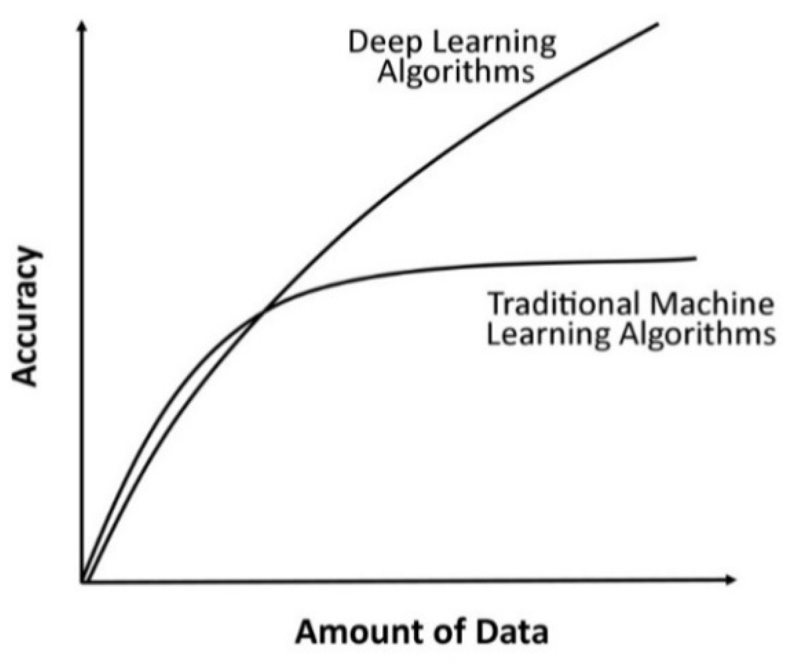
| Points of Difference | Machine Learning Models | Deep Learning Models |
|---|---|---|
| Data Requirements | Require a small amount of data for training a model. | Require a large amount of data to train a model. |
| Hardware Dependency | Machine learning algorithms can work on low-end machines such as CPUs. | Deep learning models need high-end machines for execution, such as GPUs. |
| Feature Engineering | Machine learning models rely on hand-crafted feature extractors such as Histogram of Oriented Gradients (HOG), Scale-Invariant Feature Transform (SIFT), Speeded-Up Robust Features (SURF), Principle Component Analysis (PCA), etc. for extracting features from an image. | Do not require explicit identification of features from an image. Deep learning models perform automatic feature extraction without human intervention. |
| Interpretability | Machine learning algorithms such as decision trees give crisp rules to justify why and what the algorithm chooses. Thus, it is quite easy to interpret the reasoning behind these algorithms. | It is difficult to interpret the reasoning behind deep learning algorithms. |
| Training Time | It takes less time to train a model. The time ranges from a few minutes to a few hours. The training time is dependent on data size, hardware configuration, type of model, etc. | It takes more time to train a model. The time ranges from a few hours to a few weeks. The training time is dependent on data size, hardware configuration, type of model, number of layers in a model, etc. |
| Problem Solving Technique | Divides a problem into subproblems, solves each subproblem individually, and combines results obtained from each subproblem to solve the complete problem. | Efficient in providing a solution for the complete problem. Efficient in performing both feature extraction as well as classification. |
| Preprocessing Technique | Objective(s) | Methodology | Working Mechanism | Advantages | Disadvantages |
|---|---|---|---|---|---|
| Resizing | Effective utilization of storage space and reducing computation time. | Nearest-neighbor interpolation | Replaces the value of each input pixel with the translated value nearest to it. | Simple and fast. | Causes distortion, blurring, and edge halos. |
| Bilinear interpolation | The average of four nearest pixel values is used to find the value of a new pixel. | No grey discontinuity defects and provides satisfactory results. | Produces blurring and edge halos. Time consuming and more complex than the nearest-neighbor interpolation. | ||
| Bicubic interpolation | Considers the closest 4 × 4 neighborhood of known pixels, i.e., 16 nearest neighbors of a pixel. | Provides smoother images with less interpolation distortion. | It needs more time to generate the output due to complex calculations. | ||
| Augmentation | To increase the amount of relevant data in a dataset for training a model. | Traditional augmentation techniques | Generate new data from existing data by applying various transformation techniques such as rotation, flipping, scaling, cropping, translation, adding Gaussian noise, etc. | Simple to implement. | Disadvantages of geometric transformations include additional memory, transformation compute costs, and additional training time. |
| Generative Adversarial Networks (GANs) | Comprise of a generator and a discriminator. Generator generates new examples, whereas discriminator distinguishes between generated and real. | Gives very impressive result by generating realistic visual content. | It fails to recover the texture of an image correctly. In the case of too small text or distortion in an original image, it generates a completely different image. | ||
| Neural style transfer | Combines the content of one image with the style of another to form a new image. | Generating artistic artifacts with high quality. | |||
| Normalization and Standardization | Used to find a new range of pixel values of an image. | Decimal scaling | Divides all pixel values with the largest value, i.e., 255 (8-bit RGB image). | Simplest transformation technique. | |
| Min–Max normalization | The minimum pixel value is transformed to 0; the maximum value is transformed to 1. Other values are transformed into a decimal number between 0 and 1. | It provides a uniform scale for all pixels. | It is ineffective in handling outliers. | ||
| Standardization or Z-score normalization | Standardization or Z-score normalization performs zero centering of data by subtracting the value of mean from each pixel and then dividing each dimension by its standard deviation. | It effectively handles outliers. | It does not produce normalized data with a uniform scale. | ||
| Annotation | Used for selecting objects in images and labeling the selected objects with their names. | Bounding box annotations | A rectangle superimposed over an image in which all key features of a particular object are expected to reside. | Easy to create, declared by simply specifying X and Y coordinates for the upper left and bottom right corners of the box. | Additional noise is also included in the bounded box. This method faces difficulty for occluded objects. |
| Pixel-wise image annotations | Point-by-point object selection is completed through the edges of objects. | Easy to use for any task where sizable, discrete regions must be classified/recognized. | High computation cost in terms of time. More prone to human errors. | ||
| Outlier Rejection | Ignores invalid or irrelevant images from a dataset. | OrganNet | OrganNet is a CNN model, trained on the existing image datasets (ImageNet and PlantClef) as an automatic filter for data validation. | OrganNet is more efficient than the hand-design features set. | |
| Denoising | Noise removal from an image. | Gaussian filter | Blurs an image and removes noise using a Gaussian function. | Conceptually simple, reduces noise and edge blurring. | It takes time, images are blurred as image details and edges are degraded. |
| Mean filter | It is a linear filter that replaces the center value in the window with the mean or average of all values of the pixel in the window. | Simple, easy to implement for smoothing of images. | Over-smooth images with high noise. | ||
| Median filter | It is a non-linear filter that replaces the center value in the window with the median of all values of the pixel in the window. | Reduces noise. Better than mean filter in preserving sharp edges. | Relatively costly and complex to compute. | ||
| Wiener filter | It minimizes the overall mean square error in the process of inverse filtering and noise smoothing. | It is optimal in terms of mean square error. Removes the additive noise and inverts the blurring simultaneously. | Slow to apply; blurs sharp edges. | ||
| Bilateral smoothing filter | It replaces the intensity of each pixel with a weighted average of intensity values from nearby pixels. | Preserves edges. Reduces noise. Performs smoothing. | Less efficient. |
| Architecture | Layers | Parameters | Highlights | Reference |
|---|---|---|---|---|
| AlexNet | 8 (5 Convolution + 3 Fully Connected) | 60 million | AlexNet is similar to LeNet-5, but it is deeper, contains more filters in each layer, and uses stacked convolutional layers. Winner of ILSVRC-2012. | [74] |
| VGGNet | 16–19 (13–16 convolution + 3 FC) | 134 million | The depth of a model is increased by using small convolutional filters of dimensions 3 × 3 in all layers to improve its accuracy. First runner-up in ILSVRC-2014 challenge. | [31] |
| GoogLeNet | 22 Convolution layers, 9 Inception modules | 4 million | A deeper and wider architecture with different receptive field sizes and several very small convolutions. Winner of ILSVRC-2014. | [78] |
| Inception v3 | 42 Convolution layers, 10 Inception modules | 22 million | Improves the performance of a network. It provides faster training with the use of Batch Normalization. Inception building blocks are used in an efficient way for going deeper. | [29] |
| Inception v4 | 75 Convolution layers | 41 million | Inception-v4 is considerably slower in practice due to many layers. | [108] |
| ResNet | 50 in ResNet-50, 101 in ResNet-101, 152 in ResNet-152 | 25.6 million in ResNet-50, 44.5 million in ResNet-101, 60.2 million in ResNet-152. | A novel architecture with ‘skip connections’ and heavy batch normalization. Winner of ILSVRC 2015. | [32] |
| ResNeXt-50 | 49 Convolution layers and 1 Fully Connected layer | 25 million | Use ResNeXt blocks based on the strategy of ‘split–transform–merge’. Despite creating filters for a full channel depth of input, the input is split into groups. Each group represents a channel. | [81] |
| DenseNet-121 | 117 Convolution layers, 3 Transition layers and 1 Classification layer | 27.2 million | All layers are connected directly with each other in a feed-forward manner. It reduces the vanishing-gradient problem and requires few parameters. | [33] |
| SqueezeNet | Squeeze layer and Expand layers | 50 times fewer parameters than AlexNet. | SqueezeNet is a lightweight model of size 2.9 MB. It is approximately 80 times smaller than AlexNet. Achieves the same level of accuracy as AlexNet. Reduces the number of parameters by using a smaller number of filters. | [83] |
| LeNet-5 | 7 (5 Convolution + 2 FC) | 60 thousand | Fast to deploy and efficient in solving small-scale image recognition problems. | [73] |
| Name of Optimizer | Advantages | Disadvantages |
|---|---|---|
| BGD | Easy to compute, implement and understand. | It requires large memory for calculating gradients on the whole dataset. It takes more time to converge to minima as weights are changed after calculating the gradient on the whole dataset. May trap to local minima. |
| SGD | Easy to implement. Efficient in dealing with large-scale datasets. It converges faster than batch gradient descent by frequently performing updates. It requires less memory as there is no need to store values of loss functions. | SGD requires a large number of hyper-parameters and iterations. Therefore, it is sensitive to feature scaling. It may shoot even after achieving global minima. |
| AdaGrad | Learning rate changes for each training parameter. Not required to tune the learning rate manually. It is suitable for dealing with sparse data. | The need to calculate the second-order derivative makes it expensive in terms of computation. The learning rate is constantly decreasing, which results in slow training. |
| RMSProp | A robust optimizer has pseudo curvature information. It can deal with stochastic objectives very nicely, making it applicable to min-batch learning. | The learning rate is still handcrafted. |
| Adam | Adam is very fast and converges rapidly. It resolves the vanishing learning rate problem encountered in AdaGrad. | Costly computationally. |
| Framework | Compatible Operating System | Programming Language Used for Development | Interface | Open Source | OpenMP Support | OpenCL Support | CUDA Support |
|---|---|---|---|---|---|---|---|
| TensorFlow | Linux, macOS, Windows, Android | C++, Python, CUDA | Python, Java, Go, JavaScript, R, Swift, Julia | Yes | No | Build TensorFlow with Single Source OpenCL | Yes |
| Theano | Cross-platform | Python | Python | Yes | Yes | Under development | Yes |
| Keras | Linux, macOS, Windows | Python | R, Python | Yes | Yes | TensorFlow as backend | Yes |
| Caffe | Linux, macOS, Windows | C++ | C++, MATLAB, Python | Yes | Yes | Under development | Yes |
| Torch | Linux, macOS, Windows, Android, iOS | C, Lua | Lua, LuaJIT, C, C++/OpenCL | Yes | Yes | Third-party implementations | Yes |
| deeplearning4j | Linux, macOS, Windows, Android | Java, C++ | Java, Scala, Python, Clojure, Kotlin | Yes | Yes | No | Yes |
| DL Matlab Toolbox | Linux, macOS, Windows | MATLAB, Java, C, C++ | MATLAB | No | No | No | Via GPU Coder |
| Plant | Disease | Architecture | Datasets | Results |
|---|---|---|---|---|
| Banana | Black sigatoka and Black speckle | LeNet [21] | PlantVillage: 3700 images | Accuracy: 99% |
| Apple | Black rot on Apple leaves | VGG16, VGG19, Inception-v3 and ResNet50 [18] | PlantVillage: 2086 images | VGG16: 90.4%, VGG19: 90.0%, Inception-v3: 83.0%, ResNet50: 80.0% |
| 14 different crop species | 26 different diseases | AlexNet, GoogLeNet [23] | PlantVillage: 54,306 images | AlexNet: Accuracy: 99.28% GoogLeNet: Accuracy: 99.35% |
| 6 different fruit plant species | 13 different diseases | Modified CaffeNet [25] | Authors created database containing 4483 images downloaded from the internet | Accuracy: 96.3% |
| Tomato | 9 different diseases in tomato | AlexNet, GoogLeNet [35] | PlantVillage: 14,828 Images | GoogleNet: Accuracy: 99.18% AlexNet: Accuracy: 98.66% |
| Cucumber | Melon Yellow Spot Virus (MYSV), Zucchini Yellow Mosaic Virus (ZYMV) | Author-defined CNN [36] | 800 images of cucumber leaves captured by Saitama Prefectural Agriculture and Forestry Research Center, Japan | Average accuracy: 94.9%, MYSV Sensitivity: 96.3%, ZYMV Sensitivity: 89.5%, |
| Rice | 10 different diseases | Author-defined CNN [19] | The author created a database of 500 images captured from experimental rice fields of Heilongjiang Academy of Land Reclamation Sciences, China | Accuracy: 95.48% |
| Tomato | 9 different types of diseases and pests | VGG-16, ResNet-50, ResNet-101, ResNet-152, ResNetXt-50, [82] | The author created a dataset of 5000 images captured through a camera from tomato farms located in Korea | VGG-16: 83.06%, ResNet-50: 75.37%, ResNet-101: 59.0%, ResNet-152: 66.83%, ResNetXt-50: 71.1% |
| 25 different Plant’s species | 19 different plant diseases | AlexNet, AlexNetOWTBn, GoogLeNet, Overfeat and VGGNet [24] | PlantVillage: 87,848 images of different plants (Both laboratory and field conditions) | AlexNet: 99.06%, AlexNetOWTBn: 99.49%, GoogLeNet: 92.27%, Overfeat: 98.96%, VGGNet: 99.53% |
| Apple | Mosaic, Rust, Brown spot, and Alternaria leaf spot | Authors-defined CNN architecture based on AlexNet [39] | Dataset of 13,689 synthetic images | Proposed Model: 97.62%, AlexNet: 91.19%, GoogLeNet: 95.69%, ResNet-20: 92.76%, VGGNet-16: 96.32% |
| Olive | Olive Quick Decline Syndrome (OQDS) | Authors-defined LeNet [28] | PlantVillage | Accuracy of 99% |
| Tomato | 9 different types of diseases of tomato plant | AlexNet and SqueezeNet [40] | PlantVillage | AlexNet: 95.65%, SqueezeNet: 94.3% |
| Wheat | 6 different diseases of wheat | VGG-CNN-S, VGG-CNN-VD16, VGG-FCN-S and VGG-FCN-VD16 [38] | WDD2017: 9230 wheat crop images | VGG-FCN-VD16: 97.95%, VGG-FCN-S: 95.12%, VGG-CNN-VD16: 93.27%, VGG-CNN-S: 73.00% |
| Cucumber | Anthracnose, Downy mildew, powdery mildew and Target leaf spots | Architecture similar to LeNet-5 [37] | 1184 images: PlantVillage, forestry and captured through digital camera | Proposed model: 93.4%, SVM: 81.9%, RF: 84.8%, AlexNet: 94.0% |
| Radish | Fusarium wilt | VGG-A [26] | 139 Images captured by a commercial UAV equipped with an RGB camera | Accuracy: 93.3% |
| 14 different plant species | 79 different diseases | GoogLeNet [65] | 1567 images captured using smartphones, compact cameras, DSLR cameras | Average accuracy: 94% |
| Potato | Black Scurf disease, Silver Scurf, Common Scab and Black Dot disease | VGG [22] | A total of 2465 patches of diseased potatoes | Accuracy: 96.00% |
| Tomato | Early Blight, Late Blight, Yellow Leaf Curl Virus, Spider Mite Damage and Bacterial Spot | VGG-19, Xception, Inception-v3, ResNet-50 [59] | PlantVillage: 3750 images | ResNet-50: 99.7%, Xception: 98.6%, Inception-v3: 98.4%, VGG-19: 98.2% |
| Wheat | Septoria, Tan Spot and Rust | ResNet50 [68] | Author-defined dataset of 8178 images | Accuracy: 96.00% |
| Cassava | 3 diseases: Brown leaf spot, Brown streak, and cassava mosaic 2 | Inception-v3 [104] | Author-defined dataset. Originally: 2756 images. Leaflet: 15,000 images | Accuracy: 93.00% |
| 14 different plant species | Not mentioned | VGG 16, Inception V4, ResNet50, ResNet101, ResNet152 and DenseNet121 [20] | PlantVillage | VGG16: 82%, Inception V4: 98%, ResNet50: 99.6%, ResNet101: 99.6%, ResNet152: 99.7% and DenseNet121: 99.75% |
| Maize | 8 different diseases | GoogLeNet and Cifar10 | 500 images were collected from different sources: Plant Village and Google websites | GoogLeNet: 98.9% Cifar10: 98.8% |
| Wheat | 6 different diseases | Author-defined architecture named M-bCNN (Matrix-based CNN) [85] | 16,652 images collected from Shandong Province, China | Accuracy: 90.1% |
| Maize | Northern Leaf Blight | Five CNNs were trained on the augmented data set with variations in the architecture and hyperparameters of the networks [64] | 1796 images of maize leaves grown on the Musgrave Research Farm in Aurora, NY | Accuracy: 96.7%, |
| Apple | 6 different diseases | AlexNet [106] | 2539 images of three species of apple trees from orchards located in the southern part of Brazil | Accuracy: 97.3%, |
| Radish | Fusarium wilt of radish | GoogLeNet [102] | The images were captured in Korea, including Jungsun, Gangwon, and Hongchun, using two commercial UAVs | Accuracy: 90% |
| Tomato | 8 different diseases | AlexNet, GoogLeNet, and ResNet [60] | PlantVillage: 5550 images | ResNet: 97.28% |
| Rice | Rice Blast Disease | Two CNN models similar to Lenet5 [86] | 5808 images are obtained from the Institute of Plant Protection, Jiangsu Academy of Agricultural Sciences, Nanjing, China | First CNN: 95.37% Second CNN: 95.83% |
| Banana | Five major diseases along with a pest class | ResNet50, InceptionV2, and MobileNetV1 [103] | Dataset comprises about 18,000 field images of bananas from Bioversity International, Africa, and Tamil Nadu Agricultural University, India | Accuracy between 70–90% |
| Apple, Banana | Apple scab, apple rot, banana sigotka, banana cordial leaf spot, banana diamond leaf spot, and Deightoniella leaf and fruit spot | VGG-16 [27] | 6309 sample images of apple and banana fruits PlantVillage and CASC-IFW datasets | Accuracy: 98.6% |
| Grapevine | Esca disease | LeNet-5 [77] | The dataset consists of 70,560 learning patches by the UAV system with an RGB sensor | The best results were obtained with the combination of ExR, ExG and ExGR vegetation indices using (16 × 16) patch size reaching 95.80% |
| Maize | The northern corn leaf blight, common rust and gray leaf spot | Author-defined CNN [61] | PlantVillage | Accuracy: 92.85% |
| Tea | 7 Diseases: Red leaf spot, Algal leaf spot, Bird’s eye spot, Gray blight, White spot, Anthracnose, Brown blight | Author-defined CNN model named LeafNet (Improvement over AlexNet) [84] | A total of 3810 tea leaf images captured using a Canon PowerShot G12 camera in the natural environments of Chibi and Yichang within the Hubei province of China. | Accuracy: 90.16% |
Publisher’s Note: MDPI stays neutral with regard to jurisdictional claims in published maps and institutional affiliations. |
© 2021 by the authors. Licensee MDPI, Basel, Switzerland. This article is an open access article distributed under the terms and conditions of the Creative Commons Attribution (CC BY) license (https://creativecommons.org/licenses/by/4.0/).
Share and Cite
Dhaka, V.S.; Meena, S.V.; Rani, G.; Sinwar, D.; Kavita; Ijaz, M.F.; Woźniak, M. A Survey of Deep Convolutional Neural Networks Applied for Prediction of Plant Leaf Diseases. Sensors 2021, 21, 4749. https://doi.org/10.3390/s21144749
Dhaka VS, Meena SV, Rani G, Sinwar D, Kavita, Ijaz MF, Woźniak M. A Survey of Deep Convolutional Neural Networks Applied for Prediction of Plant Leaf Diseases. Sensors. 2021; 21(14):4749. https://doi.org/10.3390/s21144749
Chicago/Turabian StyleDhaka, Vijaypal Singh, Sangeeta Vaibhav Meena, Geeta Rani, Deepak Sinwar, Kavita, Muhammad Fazal Ijaz, and Marcin Woźniak. 2021. "A Survey of Deep Convolutional Neural Networks Applied for Prediction of Plant Leaf Diseases" Sensors 21, no. 14: 4749. https://doi.org/10.3390/s21144749