Machine Learning in Agriculture: A Review


 and
and
Abstract
:1. Introduction
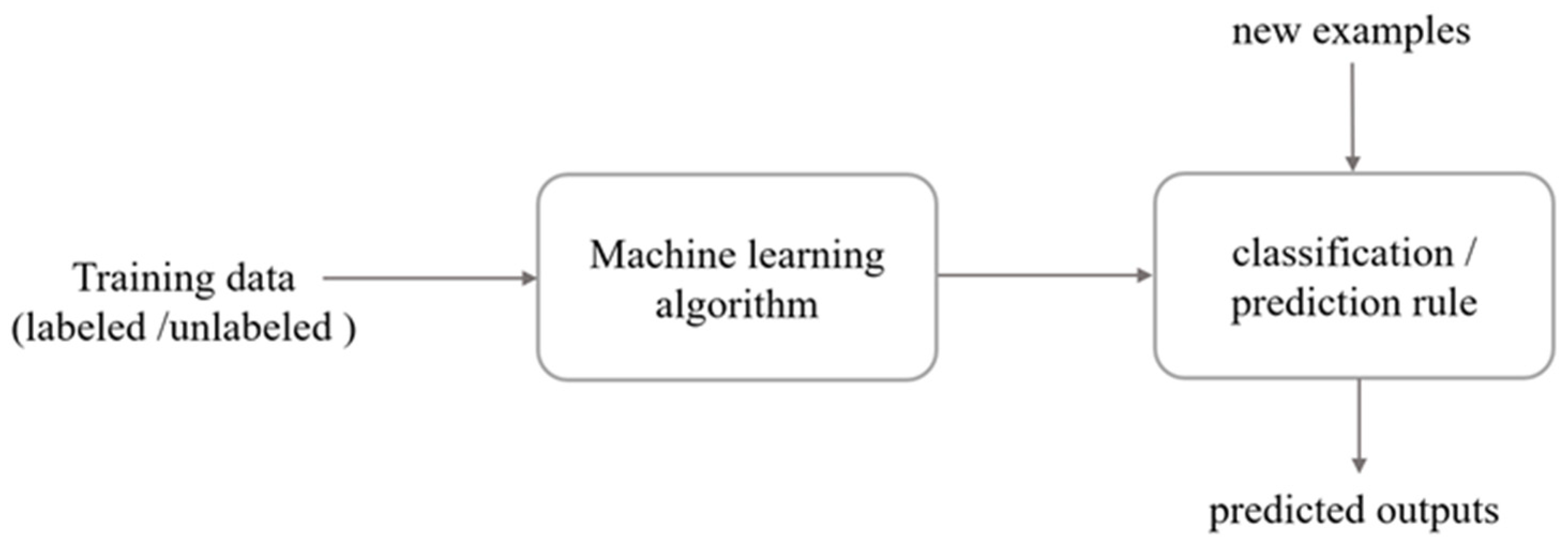
2. An Overview on Machine Learning
2.1. Machine Learning Terminology and Definitions
2.2. Tasks of Learning
2.3. Analysis of Learning
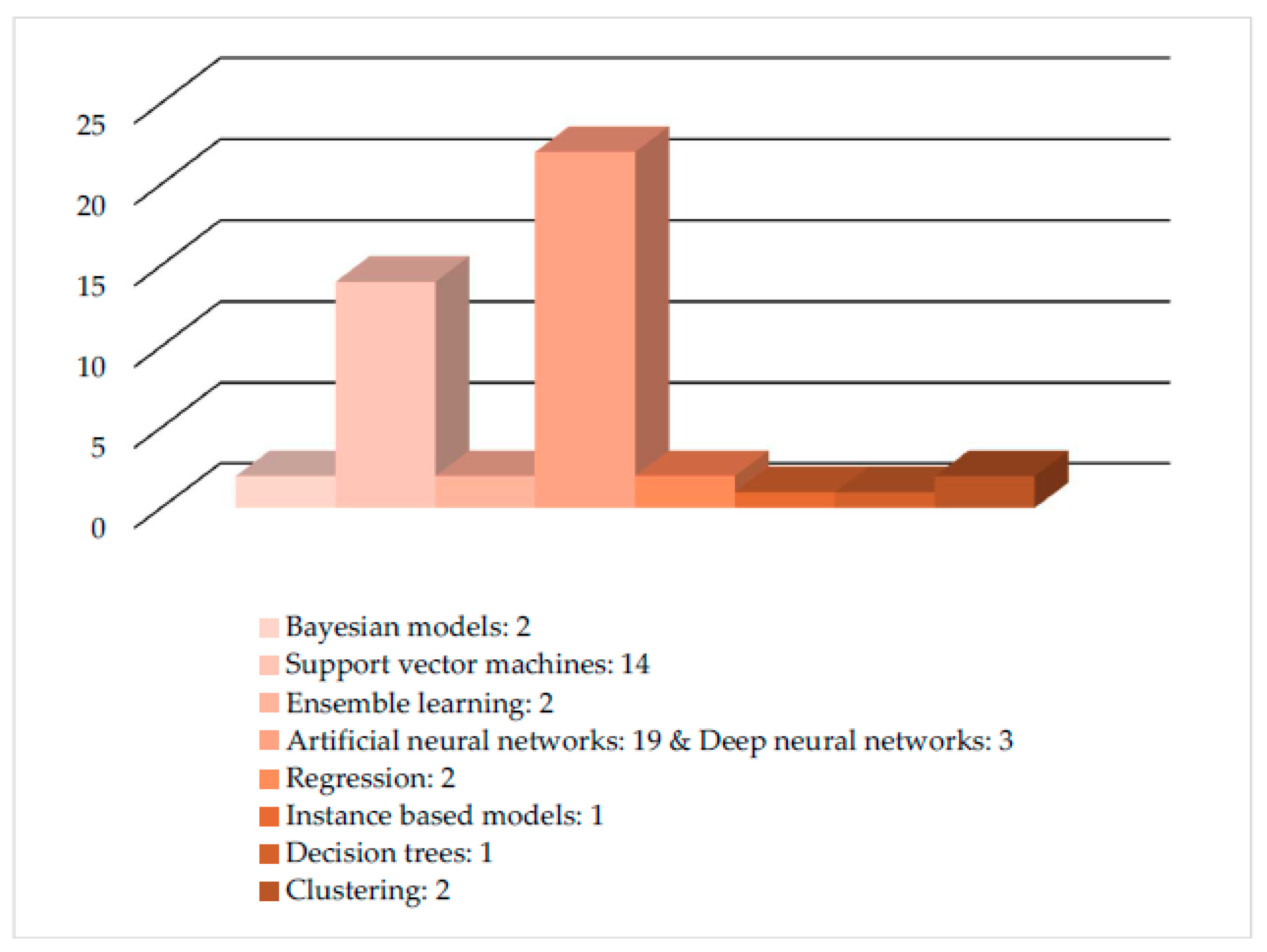
2.4. Learning Models
2.4.1. Regression
2.4.2. Clustering
2.4.3. Bayesian Models
2.4.4. Instance Based Models
2.4.5. Decision Trees
2.4.6. Artificial Neural Networks
- An input layer where the data is fed into the system,
- One or more hidden layers where the learning takes place, and
- An output layer where the decision/prediction is given.
2.4.7. Support Vector Machines
2.4.8. Ensemble Learning
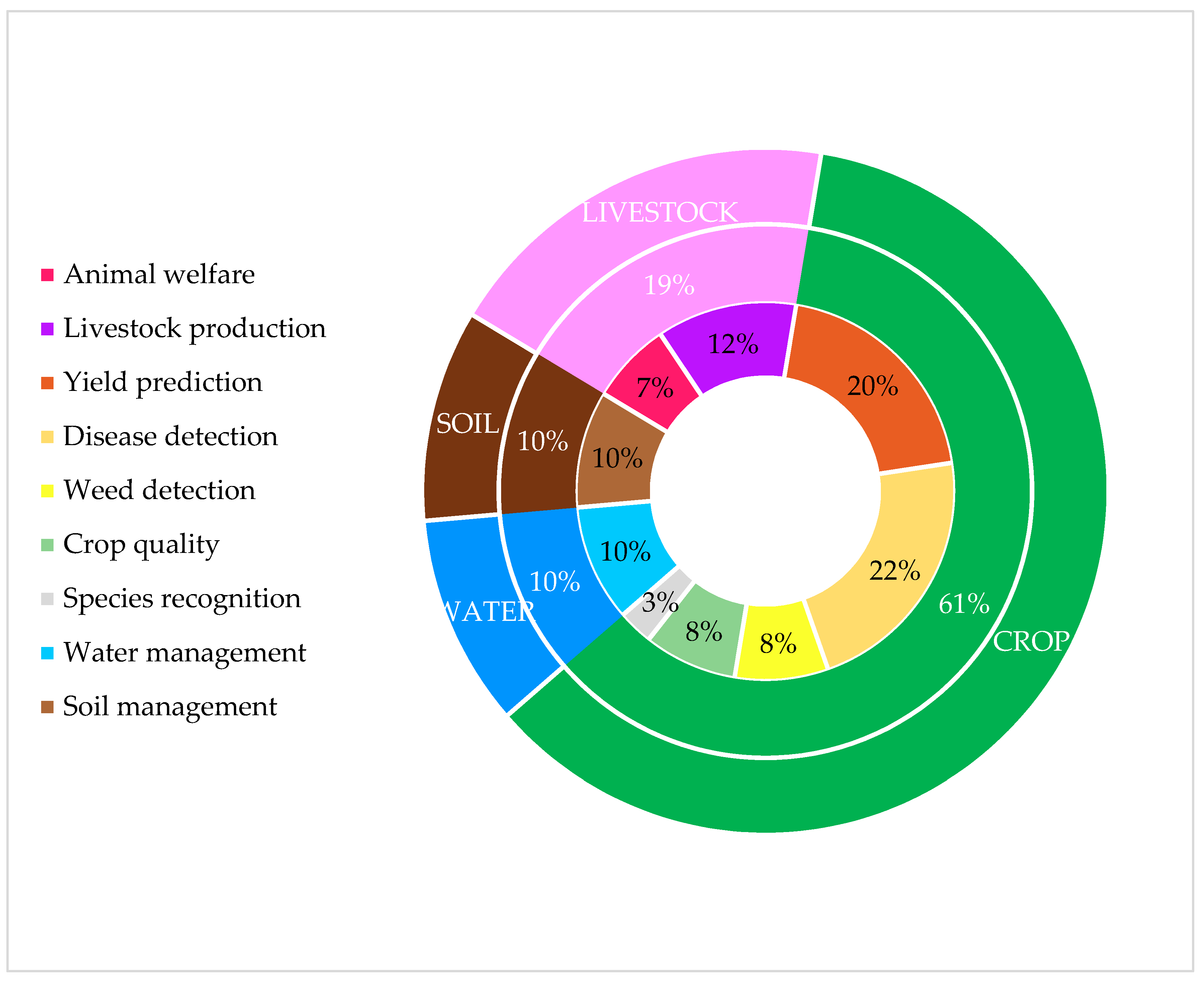
3. Review
3.1. Crop Management
3.1.1. Yield Prediction
3.1.2. Disease Detection
3.1.3. Weed Detection
3.1.4. Crop Quality
3.1.5. Species Recognition
3.2. Livestock Management
3.2.1. Animal Welfare
3.2.2. Livestock Production
3.3. Water Management
3.4. Soil Management
4. Discussion and Conclusions
Author Contributions
Funding
Conflicts of Interest
References
- Samuel, A.L. Some Studies in Machine Learning Using the Game of Checkers. IBM J. Res. Dev. 1959, 44, 206–226. [Google Scholar] [CrossRef]
- Kong, L.; Zhang, Y.; Ye, Z.Q.; Liu, X.Q.; Zhao, S.Q.; Wei, L.; Gao, G. CPC: Assess the protein-coding potential of transcripts using sequence features and support vector machine. Nucleic Acids Res. 2007, 35, 345–349. [Google Scholar] [CrossRef] [PubMed]
- Mackowiak, S.D.; Zauber, H.; Bielow, C.; Thiel, D.; Kutz, K.; Calviello, L.; Mastrobuoni, G.; Rajewsky, N.; Kempa, S.; Selbach, M.; et al. Extensive identification and analysis of conserved small ORFs in animals. Genome Biol. 2015, 16, 179. [Google Scholar] [CrossRef] [PubMed]
- Richardson, A.; Signor, B.M.; Lidbury, B.A.; Badrick, T. Clinical chemistry in higher dimensions: Machine-learning and enhanced prediction from routine clinical chemistry data. Clin. Biochem. 2016, 49, 1213–1220. [Google Scholar] [CrossRef] [PubMed]
- Wildenhain, J.; Spitzer, M.; Dolma, S.; Jarvik, N.; White, R.; Roy, M.; Griffiths, E.; Bellows, D.S.; Wright, G.D.; Tyers, M. Prediction of Synergism from Chemical-Genetic Interactions by Machine Learning. Cell Syst. 2015, 1, 383–395. [Google Scholar] [CrossRef] [PubMed]
- Kang, J.; Schwartz, R.; Flickinger, J.; Beriwal, S. Machine learning approaches for predicting radiation therapy outcomes: A clinician’s perspective. Int. J. Radiat. Oncol. Biol. Phys. 2015, 93, 1127–1135. [Google Scholar] [CrossRef] [PubMed]
- Asadi, H.; Dowling, R.; Yan, B.; Mitchell, P. Machine learning for outcome prediction of acute ischemic stroke post intra-arterial therapy. PLoS ONE 2014, 9, e88225. [Google Scholar] [CrossRef] [PubMed]
- Zhang, B.; He, X.; Ouyang, F.; Gu, D.; Dong, Y.; Zhang, L.; Mo, X.; Huang, W.; Tian, J.; Zhang, S. Radiomic machine-learning classifiers for prognostic biomarkers of advanced nasopharyngeal carcinoma. Cancer Lett. 2017, 403, 21–27. [Google Scholar] [CrossRef] [PubMed]
- Cramer, S.; Kampouridis, M.; Freitas, A.A.; Alexandridis, A.K. An extensive evaluation of seven machine learning methods for rainfall prediction in weather derivatives. Expert Syst. Appl. 2017, 85, 169–181. [Google Scholar] [CrossRef] [Green Version]
- Rhee, J.; Im, J. Meteorological drought forecasting for ungauged areas based on machine learning: Using long-range climate forecast and remote sensing data. Agric. For. Meteorol. 2017, 237–238, 105–122. [Google Scholar] [CrossRef]
- Aybar-Ruiz, A.; Jiménez-Fernández, S.; Cornejo-Bueno, L.; Casanova-Mateo, C.; Sanz-Justo, J.; Salvador-González, P.; Salcedo-Sanz, S. A novel Grouping Genetic Algorithm-Extreme Learning Machine approach for global solar radiation prediction from numerical weather models inputs. Sol. Energy 2016, 132, 129–142. [Google Scholar] [CrossRef]
- Barboza, F.; Kimura, H.; Altman, E. Machine learning models and bankruptcy prediction. Expert Syst. Appl. 2017, 83, 405–417. [Google Scholar] [CrossRef]
- Zhao, Y.; Li, J.; Yu, L. A deep learning ensemble approach for crude oil price forecasting. Energy Econ. 2017, 66, 9–16. [Google Scholar] [CrossRef]
- Bohanec, M.; Kljajić Borštnar, M.; Robnik-Šikonja, M. Explaining machine learning models in sales predictions. Expert Syst. Appl. 2017, 71, 416–428. [Google Scholar] [CrossRef]
- Takahashi, K.; Kim, K.; Ogata, T.; Sugano, S. Tool-body assimilation model considering grasping motion through deep learning. Rob. Auton. Syst. 2017, 91, 115–127. [Google Scholar] [CrossRef]
- Gastaldo, P.; Pinna, L.; Seminara, L.; Valle, M.; Zunino, R. A tensor-based approach to touch modality classification by using machine learning. Rob. Auton. Syst. 2015, 63, 268–278. [Google Scholar] [CrossRef]
- López-Cortés, X.A.; Nachtigall, F.M.; Olate, V.R.; Araya, M.; Oyanedel, S.; Diaz, V.; Jakob, E.; Ríos-Momberg, M.; Santos, L.S. Fast detection of pathogens in salmon farming industry. Aquaculture 2017, 470, 17–24. [Google Scholar] [CrossRef]
- Zhou, C.; Lin, K.; Xu, D.; Chen, L.; Guo, Q.; Sun, C.; Yang, X. Near infrared computer vision and neuro-fuzzy model-based feeding decision system for fish in aquaculture. Comput. Electron. Agric. 2018, 146, 114–124. [Google Scholar] [CrossRef]
- Fragni, R.; Trifirò, A.; Nucci, A.; Seno, A.; Allodi, A.; Di Rocco, M. Italian tomato-based products authentication by multi-element approach: A mineral elements database to distinguish the domestic provenance. Food Control 2018, 93, 211–218. [Google Scholar] [CrossRef]
- Maione, C.; Barbosa, R.M. Recent applications of multivariate data analysis methods in the authentication of rice and the most analyzed parameters: A review. Crit. Rev. Food Sci. Nutr. 2018, 1–12. [Google Scholar] [CrossRef] [PubMed]
- Fang, K.; Shen, C.; Kifer, D.; Yang, X. Prolongation of SMAP to Spatiotemporally Seamless Coverage of Continental U.S. Using a Deep Learning Neural Network. Geophys. Res. Lett. 2017, 44, 11030–11039. [Google Scholar] [CrossRef]
- Pearson, K. On lines and planes of closest fit to systems of points in space. Lond. Edinb. Dublin Philos. Mag. J. Sci. 1901, 2, 559–572. [Google Scholar] [CrossRef]
- Wold, H. Partial Least Squares. In Encyclopedia of Statistical Sciences; John Wiley & Sons: Chichester, NY, USA, 1985; Volume 6, pp. 581–591. ISBN 9788578110796. [Google Scholar]
- Fisher, R.A. The use of multiple measures in taxonomic problems. Ann. Eugen. 1936, 7, 179–188. [Google Scholar] [CrossRef]
- Cox, D.R. The Regression Analysis of Binary Sequences. J. R. Stat. Soc. Ser. B 1958, 20, 215–242. [Google Scholar] [CrossRef]
- Efroymson, M.A. Multiple regression analysis. Math. Methods Digit. Comput. 1960, 1, 191–203. [Google Scholar] [CrossRef]
- Craven, B.D.; Islam, S.M.N. Ordinary least-squares regression. SAGE Dict. Quant. Manag. Res. 2011, 224–228. [Google Scholar]
- Friedman, J.H. Multivariate Adaptive Regression Splines. Ann. Stat. 1991, 19, 1–67. [Google Scholar] [CrossRef] [Green Version]
- Quinlan, J.R. Learning with continuous classes. Mach. Learn. 1992, 92, 343–348. [Google Scholar]
- Cleveland, W.S. Robust locally weighted regression and smoothing scatterplots. J. Am. Stat. Assoc. 1979, 74, 829–836. [Google Scholar] [CrossRef]
- Tryon, R.C. Communality of a variable: Formulation by cluster analysis. Psychometrika 1957, 22, 241–260. [Google Scholar] [CrossRef]
- Lloyd, S.P. Least Squares Quantization in PCM. IEEE Trans. Inf. Theory 1982, 28, 129–137. [Google Scholar] [CrossRef]
- Johnson, S.C. Hierarchical clustering schemes. Psychometrika 1967, 32, 241–254. [Google Scholar] [CrossRef] [PubMed]
- Dempster, A.P.; Laird, N.M.; Rubin, D.B. Maximum likelihood from incomplete data via the EM algorithm. J. R. Stat. Soc. Ser. B Methodol. 1977, 39, 1–38. [Google Scholar] [CrossRef]
- Russell, S.J.; Norvig, P. Artificial Intelligence: A Modern Approach; Prentice Hall: Upper Saddle River, NJ, USA, 1995; Volume 9, ISBN 9780131038059. [Google Scholar]
- Pearl, J. Probabilistic Reasoning in Intelligent Systems. Morgan Kauffmann San Mateo 1988, 88, 552. [Google Scholar]
- Duda, R.O.; Hart, P.E. Pattern Classification and Scene Analysis; Wiley: Hoboken, NJ, USA, 1973; Volume 7, ISBN 0471223611. [Google Scholar]
- Neapolitan, R.E. Models for reasoning under uncertainty. Appl. Artif. Intell. 1987, 1, 337–366. [Google Scholar] [CrossRef]
- Fix, E.; Hodges, J.L. Discriminatory Analysis–Nonparametric discrimination consistency properties. Int. Stat. Rev. 1951, 57, 238–247. [Google Scholar] [CrossRef]
- Atkeson, C.G.; Moorey, A.W.; Schaalz, S.; Moore, A.W.; Schaal, S. Locally Weighted Learning. Artif. Intell. 1997, 11, 11–73. [Google Scholar] [CrossRef]
- Kohonen, T. Learning vector quantization. Neural Netw. 1988, 1, 303. [Google Scholar] [CrossRef]
- Belson, W.A. Matching and Prediction on the Principle of Biological Classification. Appl. Stat. 1959, 8, 65–75. [Google Scholar] [CrossRef]
- Breiman, L.; Friedman, J.H.; Olshen, R.A.; Stone, C.J. Classification and Regression Trees; Routledge: Abingdon, UK, 1984; Volume 19, ISBN 0412048418. [Google Scholar]
- Kass, G.V. An Exploratory Technique for Investigating Large Quantities of Categorical Data. Appl. Stat. 1980, 29, 119. [Google Scholar] [CrossRef]
- Quinlan, J.R. C4.5: Programs for Machine Learning; Morgan Kaufmann Publishers Inc.: San Francisco, CA, USA, 1992; Volume 1, ISBN 1558602380. [Google Scholar]
- McCulloch, W.S.; Pitts, W. A logical calculus of the ideas immanent in nervous activity. Bull. Math. Biophys. 1943, 5, 115–133. [Google Scholar] [CrossRef]
- Broomhead, D.S.; Lowe, D. Multivariable Functional Interpolation and Adaptive Networks. Complex Syst. 1988, 2, 321–355. [Google Scholar]
- Rosenblatt, F. The perceptron: A probabilistic model for information storage and organization in the brain. Psychol. Rev. 1958, 65, 386–408. [Google Scholar] [CrossRef] [PubMed]
- Linnainmaa, S. Taylor expansion of the accumulated rounding error. BIT 1976, 16, 146–160. [Google Scholar] [CrossRef]
- Riedmiller, M.; Braun, H. A direct adaptive method for faster backpropagation learning: The RPROP algorithm. In Proceedings of the IEEE International Conference on Neural Networks, San Francisco, CA, USA, 28 March–1 April 1993; pp. 586–591. [Google Scholar] [CrossRef]
- Hecht-Nielsen, R. Counterpropagation networks. Appl. Opt. 1987, 26, 4979–4983. [Google Scholar] [CrossRef] [PubMed]
- Jang, J.S.R. ANFIS: Adaptive-Network-Based Fuzzy Inference System. IEEE Trans. Syst. Man Cybern. 1993, 23, 665–685. [Google Scholar] [CrossRef]
- Melssen, W.; Wehrens, R.; Buydens, L. Supervised Kohonen networks for classification problems. Chemom. Intell. Lab. Syst. 2006, 83, 99–113. [Google Scholar] [CrossRef]
- Hopfield, J.J. Neural networks and physical systems with emergent collective computational abilities. Proc. Natl. Acad. Sci. USA 1982, 79, 2554–2558. [Google Scholar] [CrossRef] [PubMed]
- Pal, S.K.; Mitra, S. Multilayer Perceptron, Fuzzy Sets, and Classification. IEEE Trans. Neural Netw. 1992, 3, 683–697. [Google Scholar] [CrossRef] [PubMed]
- Kohonen, T. The Self-Organizing Map. Proc. IEEE 1990, 78, 1464–1480. [Google Scholar] [CrossRef]
- Huang, G.-B.; Zhu, Q.-Y.; Siew, C.-K. Extreme learning machine: Theory and applications. Neurocomputing 2006, 70, 489–501. [Google Scholar] [CrossRef] [Green Version]
- Specht, D.F. A general regression neural network. IEEE Trans. Neural Netw. 1991, 2, 568–576. [Google Scholar] [CrossRef] [PubMed]
- Cao, J.; Lin, Z.; Huang, G. Bin Self-adaptive evolutionary extreme learning machine. Neural Process. Lett. 2012, 36, 285–305. [Google Scholar] [CrossRef]
- LeCun, Y.; Bengio, Y.; Hinton, G. Deep learning. Nature 2015, 521, 436–444. [Google Scholar] [CrossRef] [PubMed]
- Goodfellow, I.; Bengio, Y.; Courville, A. Deep Learning; MIT Press: Cambridge, MA, USA, 2016; pp. 216–261. [Google Scholar]
- Salakhutdinov, R.; Hinton, G. Deep Boltzmann Machines. Aistats 2009, 1, 448–455. [Google Scholar] [CrossRef]
- Vincent, P.; Larochelle, H.; Lajoie, I.; Bengio, Y.; Manzagol, P.-A. Stacked Denoising Autoencoders: Learning Useful Representations in a Deep Network with a Local Denoising Criterion Pierre-Antoine Manzagol. J. Mach. Learn. Res. 2010, 11, 3371–3408. [Google Scholar] [CrossRef]
- Vapnik, V. Support vector machine. Mach. Learn. 1995, 20, 273–297. [Google Scholar]
- Suykens, J.A.K.; Vandewalle, J. Least Squares Support Vector Machine Classifiers. Neural Process. Lett. 1999, 9, 293–300. [Google Scholar] [CrossRef]
- Chang, C.; Lin, C. LIBSVM: A Library for Support Vector Machines. ACM Trans. Intell. Syst. Technol. 2013, 2, 1–39. [Google Scholar] [CrossRef]
- Smola, A. Regression Estimation with Support Vector Learning Machines. Master’s Thesis, The Technical University of Munich, Munich, Germany, 1996; pp. 1–78. [Google Scholar]
- Suykens, J.A.K.; Van Gestel, T.; De Brabanter, J.; De Moor, B.; Vandewalle, J. Least Squares Support Vector Machines; World Scientific: Singapore, 2002; ISBN 9812381511. [Google Scholar]
- Galvão, R.K.H.; Araújo, M.C.U.; Fragoso, W.D.; Silva, E.C.; José, G.E.; Soares, S.F.C.; Paiva, H.M. A variable elimination method to improve the parsimony of MLR models using the successive projections algorithm. Chemom. Intell. Lab. Syst. 2008, 92, 83–91. [Google Scholar] [CrossRef]
- Breiman, L. Random Forests. Mach. Learn. 2001, 45, 5–32. [Google Scholar] [CrossRef] [Green Version]
- Schapire, R.E. A brief introduction to boosting. In Proceedings of the IJCAI International Joint Conference on Artificial Intelligence, Stockholm, Sweden, 31 July–6 August 1999; Volume 2, pp. 1401–1406. [Google Scholar]
- Freund, Y.; Schapire, R.E. Experiments with a New Boosting Algorithm. In Proceedings of the Thirteenth International Conference on International Conference on Machine Learning, Bari, Italy, 3–6 July 1996; Morgan Kaufmann Publishers Inc.: San Francisco, CA, USA, 1996; pp. 148–156. [Google Scholar]
- Breiman, L. Bagging Predictors. Mach. Learn. 1996, 24, 123–140. [Google Scholar] [CrossRef]
- Ramos, P.J.; Prieto, F.A.; Montoya, E.C.; Oliveros, C.E. Automatic fruit count on coffee branches using computer vision. Comput. Electron. Agric. 2017, 137, 9–22. [Google Scholar] [CrossRef]
- Amatya, S.; Karkee, M.; Gongal, A.; Zhang, Q.; Whiting, M.D. Detection of cherry tree branches with full foliage in planar architecture for automated sweet-cherry harvesting. Biosyst. Eng. 2015, 146, 3–15. [Google Scholar] [CrossRef]
- Sengupta, S.; Lee, W.S. Identification and determination of the number of immature green citrus fruit in a canopy under different ambient light conditions. Biosyst. Eng. 2014, 117, 51–61. [Google Scholar] [CrossRef]
- Ali, I.; Cawkwell, F.; Dwyer, E.; Green, S. Modeling Managed Grassland Biomass Estimation by Using Multitemporal Remote Sensing Data—A Machine Learning Approach. IEEE J. Sel. Top. Appl. Earth Obs. Remote Sens. 2016, 10, 3254–3264. [Google Scholar] [CrossRef]
- Pantazi, X.-E.; Moshou, D.; Alexandridis, T.K.; Whetton, R.L.; Mouazen, A.M. Wheat yield prediction using machine learning and advanced sensing techniques. Comput. Electron. Agric. 2016, 121, 57–65. [Google Scholar] [CrossRef]
- Senthilnath, J.; Dokania, A.; Kandukuri, M.; Ramesh, K.N.; Anand, G.; Omkar, S.N. Detection of tomatoes using spectral-spatial methods in remotely sensed RGB images captured by UAV. Biosyst. Eng. 2016, 146, 16–32. [Google Scholar] [CrossRef]
- Su, Y.; Xu, H.; Yan, L. Support vector machine-based open crop model (SBOCM): Case of rice production in China. Saudi J. Biol. Sci. 2017, 24, 537–547. [Google Scholar] [CrossRef] [PubMed]
- Kung, H.-Y.; Kuo, T.-H.; Chen, C.-H.; Tsai, P.-Y. Accuracy Analysis Mechanism for Agriculture Data Using the Ensemble Neural Network Method. Sustainability 2016, 8, 735. [Google Scholar] [CrossRef]
- Pantazi, X.E.; Tamouridou, A.A.; Alexandridis, T.K.; Lagopodi, A.L.; Kontouris, G.; Moshou, D. Detection of Silybum marianum infection with Microbotryum silybum using VNIR field spectroscopy. Comput. Electron. Agric. 2017, 137, 130–137. [Google Scholar] [CrossRef]
- Ebrahimi, M.A.; Khoshtaghaza, M.H.; Minaei, S.; Jamshidi, B. Vision-based pest detection based on SVM classification method. Comput. Electron. Agric. 2017, 137, 52–58. [Google Scholar] [CrossRef]
- Chung, C.L.; Huang, K.J.; Chen, S.Y.; Lai, M.H.; Chen, Y.C.; Kuo, Y.F. Detecting Bakanae disease in rice seedlings by machine vision. Comput. Electron. Agric. 2016, 121, 404–411. [Google Scholar] [CrossRef]
- Pantazi, X.E.; Moshou, D.; Oberti, R.; West, J.; Mouazen, A.M.; Bochtis, D. Detection of biotic and abiotic stresses in crops by using hierarchical self organizing classifiers. Precis. Agric. 2017, 18, 383–393. [Google Scholar] [CrossRef]
- Moshou, D.; Pantazi, X.-E.; Kateris, D.; Gravalos, I. Water stress detection based on optical multisensor fusion with a least squares support vector machine classifier. Biosyst. Eng. 2014, 117, 15–22. [Google Scholar] [CrossRef]
- Moshou, D.; Bravo, C.; West, J.; Wahlen, S.; McCartney, A.; Ramon, H. Automatic detection of “yellow rust” in wheat using reflectance measurements and neural networks. Comput. Electron. Agric. 2004, 44, 173–188. [Google Scholar] [CrossRef]
- Moshou, D.; Bravo, C.; Oberti, R.; West, J.; Bodria, L.; McCartney, A.; Ramon, H. Plant disease detection based on data fusion of hyper-spectral and multi-spectral fluorescence imaging using Kohonen maps. Real-Time Imaging 2005, 11, 75–83. [Google Scholar] [CrossRef]
- Moshou, D.; Bravo, C.; Wahlen, S.; West, J.; McCartney, A.; De Baerdemaeker, J.; Ramon, H. Simultaneous identification of plant stresses and diseases in arable crops using proximal optical sensing and self-organising maps. Precis. Agric. 2006, 7, 149–164. [Google Scholar] [CrossRef]
- Ferentinos, K.P. Deep learning models for plant disease detection and diagnosis. Comput. Electron. Agric. 2018, 145, 311–318. [Google Scholar] [CrossRef]
- Pantazi, X.E.; Tamouridou, A.A.; Alexandridis, T.K.; Lagopodi, A.L.; Kashefi, J.; Moshou, D. Evaluation of hierarchical self-organising maps for weed mapping using UAS multispectral imagery. Comput. Electron. Agric. 2017, 139, 224–230. [Google Scholar] [CrossRef]
- Pantazi, X.-E.; Moshou, D.; Bravo, C. Active learning system for weed species recognition based on hyperspectral sensing. Biosyst. Eng. 2016, 146, 193–202. [Google Scholar] [CrossRef]
- Binch, A.; Fox, C.W. Controlled comparison of machine vision algorithms for Rumex and Urtica detection in grassland. Comput. Electron. Agric. 2017, 140, 123–138. [Google Scholar] [CrossRef] [Green Version]
- Zhang, M.; Li, C.; Yang, F. Classification of foreign matter embedded inside cotton lint using short wave infrared (SWIR) hyperspectral transmittance imaging. Comput. Electron. Agric. 2017, 139, 75–90. [Google Scholar] [CrossRef]
- Hu, H.; Pan, L.; Sun, K.; Tu, S.; Sun, Y.; Wei, Y.; Tu, K. Differentiation of deciduous-calyx and persistent-calyx pears using hyperspectral reflectance imaging and multivariate analysis. Comput. Electron. Agric. 2017, 137, 150–156. [Google Scholar] [CrossRef]
- Maione, C.; Batista, B.L.; Campiglia, A.D.; Barbosa, F.; Barbosa, R.M. Classification of geographic origin of rice by data mining and inductively coupled plasma mass spectrometry. Comput. Electron. Agric. 2016, 121, 101–107. [Google Scholar] [CrossRef]
- Grinblat, G.L.; Uzal, L.C.; Larese, M.G.; Granitto, P.M. Deep learning for plant identification using vein morphological patterns. Comput. Electron. Agric. 2016, 127, 418–424. [Google Scholar] [CrossRef]
- Dutta, R.; Smith, D.; Rawnsley, R.; Bishop-Hurley, G.; Hills, J.; Timms, G.; Henry, D. Dynamic cattle behavioural classification using supervised ensemble classifiers. Comput. Electron. Agric. 2015, 111, 18–28. [Google Scholar] [CrossRef]
- Pegorini, V.; Karam, L.Z.; Pitta, C.S.R.; Cardoso, R.; da Silva, J.C.C.; Kalinowski, H.J.; Ribeiro, R.; Bertotti, F.L.; Assmann, T.S. In vivo pattern classification of ingestive behavior in ruminants using FBG sensors and machine learning. Sensors 2015, 15, 28456–28471. [Google Scholar] [CrossRef] [PubMed]
- Matthews, S.G.; Miller, A.L.; PlÖtz, T.; Kyriazakis, I. Automated tracking to measure behavioural changes in pigs for health and welfare monitoring. Sci. Rep. 2017, 7, 17582. [Google Scholar] [CrossRef] [PubMed] [Green Version]
- Craninx, M.; Fievez, V.; Vlaeminck, B.; De Baets, B. Artificial neural network models of the rumen fermentation pattern in dairy cattle. Comput. Electron. Agric. 2008, 60, 226–238. [Google Scholar] [CrossRef]
- Morales, I.R.; Cebrián, D.R.; Fernandez-Blanco, E.; Sierra, A.P. Early warning in egg production curves from commercial hens: A SVM approach. Comput. Electron. Agric. 2016, 121, 169–179. [Google Scholar] [CrossRef]
- Alonso, J.; Villa, A.; Bahamonde, A. Improved estimation of bovine weight trajectories using Support Vector Machine Classification. Comput. Electron. Agric. 2015, 110, 36–41. [Google Scholar] [CrossRef] [Green Version]
- Alonso, J.; Castañón, Á.R.; Bahamonde, A. Support Vector Regression to predict carcass weight in beef cattle in advance of the slaughter. Comput. Electron. Agric. 2013, 91, 116–120. [Google Scholar] [CrossRef] [Green Version]
- Hansen, M.F.; Smith, M.L.; Smith, L.N.; Salter, M.G.; Baxter, E.M.; Farish, M.; Grieve, B. Towards on-farm pig face recognition using convolutional neural networks. Comput. Ind. 2018, 98, 145–152. [Google Scholar] [CrossRef]
- Mehdizadeh, S.; Behmanesh, J.; Khalili, K. Using MARS, SVM, GEP and empirical equations for estimation of monthly mean reference evapotranspiration. Comput. Electron. Agric. 2017, 139, 103–114. [Google Scholar] [CrossRef]
- Feng, Y.; Peng, Y.; Cui, N.; Gong, D.; Zhang, K. Modeling reference evapotranspiration using extreme learning machine and generalized regression neural network only with temperature data. Comput. Electron. Agric. 2017, 136, 71–78. [Google Scholar] [CrossRef]
- Patil, A.P.; Deka, P.C. An extreme learning machine approach for modeling evapotranspiration using extrinsic inputs. Comput. Electron. Agric. 2016, 121, 385–392. [Google Scholar] [CrossRef]
- Mohammadi, K.; Shamshirband, S.; Motamedi, S.; Petković, D.; Hashim, R.; Gocic, M. Extreme learning machine based prediction of daily dew point temperature. Comput. Electron. Agric. 2015, 117, 214–225. [Google Scholar] [CrossRef]
- Coopersmith, E.J.; Minsker, B.S.; Wenzel, C.E.; Gilmore, B.J. Machine learning assessments of soil drying for agricultural planning. Comput. Electron. Agric. 2014, 104, 93–104. [Google Scholar] [CrossRef]
- Morellos, A.; Pantazi, X.-E.; Moshou, D.; Alexandridis, T.; Whetton, R.; Tziotzios, G.; Wiebensohn, J.; Bill, R.; Mouazen, A.M. Machine learning based prediction of soil total nitrogen, organic carbon and moisture content by using VIS-NIR spectroscopy. Biosyst. Eng. 2016, 152, 104–116. [Google Scholar] [CrossRef]
- Nahvi, B.; Habibi, J.; Mohammadi, K.; Shamshirband, S.; Al Razgan, O.S. Using self-adaptive evolutionary algorithm to improve the performance of an extreme learning machine for estimating soil temperature. Comput. Electron. Agric. 2016, 124, 150–160. [Google Scholar] [CrossRef]
- Johann, A.L.; de Araújo, A.G.; Delalibera, H.C.; Hirakawa, A.R. Soil moisture modeling based on stochastic behavior of forces on a no-till chisel opener. Comput. Electron. Agric. 2016, 121, 420–428. [Google Scholar] [CrossRef]


| Abbreviation | Model |
|---|---|
| ANNs | artificial neural networks |
| BM | bayesian models |
| DL | deep learning |
| DR | dimensionality reduction |
| DT | decision trees |
| EL | ensemble learning |
| IBM | instance based models |
| SVMs | support vector machines |
| Abbreviation | Algorithm |
|---|---|
| ANFIS | adaptive-neuro fuzzy inference systems |
| Bagging | bootstrap aggregating |
| BBN | bayesian belief network |
| BN | bayesian network |
| BPN | back-propagation network |
| CART | classification and regression trees |
| CHAID | chi-square automatic interaction detector |
| CNNs | convolutional neural networks |
| CP | counter propagation |
| DBM | deep boltzmann machine |
| DBN | deep belief network |
| DNN | deep neural networks |
| ELMs | extreme learning machines |
| EM | expectation maximisation |
| ENNs | ensemble neural networks |
| GNB | gaussian naive bayes |
| GRNN | generalized regression neural network |
| KNN | k-nearest neighbor |
| LDA | linear discriminant analysis |
| LS-SVM | least squares-support vector machine |
| LVQ | learning vector quantization |
| LWL | locally weighted learning |
| MARS | multivariate adaptive regression splines |
| MLP | multi-layer perceptron |
| MLR | multiple linear regression |
| MOG | mixture of gaussians |
| OLSR | ordinary least squares regression |
| PCA | principal component analysis |
| PLSR | partial least squares regression |
| RBFN | radial basis function networks |
| RF | random forest |
| SaE-ELM | self adaptive evolutionary-extreme learning machine |
| SKNs | supervised kohonen networks |
| SOMs | self-organising maps |
| SPA-SVM | successive projection algorithm-support vector machine |
| SVR | support vector regression |
| Abbreviation | Measure |
|---|---|
| APE | average prediction error |
| MABE | mean absolute bias error |
| MAE | mean absolute error |
| MAPE | mean absolute percentage error |
| MPE | mean percentage error |
| NS | nash-sutcliffe coefficient |
| R | radius |
| R2 | coefficient of determination |
| RMSE | root mean squared error |
| RMSEP | root mean square error of prediction |
| RPD | relative percentage difference |
| RRMSE | average relative root mean square error |
| Abbreviation | |
|---|---|
| AUS | aircraft unmanned system |
| Cd | cadmium |
| FBG | fiber bragg grating |
| HSV | hue saturation value color space |
| K | potassium |
| MC | moisture content |
| Mg | magnesium |
| ML | machine learning |
| NDVI | normalized difference vegetation index |
| NIR | near infrared |
| OC | organic carbon |
| Rb | rubidium |
| RGB | red green blue |
| TN | total nitrogen |
| UAV | unmanned aerial vehicle |
| VIS-NIR | visible-near infrared |
| Article | Crop | Observed Features | Functionality | Models/Algorithms | Results |
|---|---|---|---|---|---|
| [74] | Coffee | Forty-two (42) color features in digital images illustrating coffee fruits | Automatic count of coffee fruits on a coffee branch | SVM | Harvestable:
|
| [75] | Cherry | Colored digital images depicting leaves, branches, cherry fruits, and the background | Detection of cherry branches with full foliage | BM/GNB | 89.6% accuracy |
| [76] | Green citrus | Image features (form 20 × 20 pixels digital images of unripe green citrus fruits) such as coarseness, contrast, directionality, line-likeness, regularity, roughness, granularity, irregularity, brightness, smoothness, and fineness | Identification of the number of immature green citrus fruit under natural outdoor conditions | SVM | 80.4% accuracy |
| [77] | Grass | Vegetation indices, spectral bands of red and NIR | Estimation of grassland biomass (kg dry matter/ha/day) for two managed grassland farms in Ireland; Moorepark and Grange | ANN/ANFIS | Moorepark: R2 = 0.85 RMSE = 11.07 Grange: R2 = 0.76 RMSE = 15.35 |
| [78] | Wheat | Normalized values of on-line predicted soil parameters and the satellite NDVI | Wheat yield prediction within field variation | ANN/SNKs | 81.65% accuracy |
| [79] | Tomato | High spatial resolution RGB images | Detection of tomatoes via RGB images captured by UAV | Clustering/EM | Recall: 0.6066 Precision: 0.9191 F-Measure: 0.7308 |
| [80] | Rice | Agricultural, surface weather, and soil physico-chemical data with yield or development records | Rice development stage prediction and yield prediction | SVM | Middle-season rice: Tillering stage: RMSE (kg h−1 m2) = 126.8 Heading stage: RMSE (kg h−1 m2) = 96.4 Milk stage: RMSE (kg h−1 m2) = 109.4 Early rice: Tillering stage: RMSE (kg h−1 m2) = 88.3 Heading stage: RMSE (kg h−1 m2) = 68.0 Milk stage: RMSE (kg h−1 m2) = 36.4 Late rice: Tillering stage: RMSE (kg h−1 m2) = 89.2 Heading stage: RMSE (kg h−1 m2) = 69.7 Milk stage: RMSE (kg h−1 m2) = 46.5 |
| [81] | General | Agriculture data: meteorological, environmental, economic, and harvest | Method for the accurate analysis for agricultural yield predictions | ANN/ENN and BPN based | 1.3% error rate |
| Author | Crop | Observed Features | Functionality | Models/Algorithms | Results |
|---|---|---|---|---|---|
| [82] | Silybum marianum | Images with leaf spectra using a handheld visible and NIR spectrometer | Detection and discrimination between healthy Silybum marianum plants and those that are infected by smut fungus Microbotyum silybum | ANN/XY-Fusion | 95.16% accuracy |
| [83] | Strawberry | Region index: ratio of major diameter to minor diameter; and color indexes: hue, saturation, and intensify | Classification of parasites and automatic detection of thrips | SVM | MPE = 2.25% |
| [84] | Rice | Morphological and color traits from healthy and infected from Bakanae disease, rice seedlings, for cultivars Tainan 11 and Toyonishiki | Detection of Bakanae disease, Fusarium fujikuroi, in rice seedlings | SVM | 87.9% accuracy |
| [85] | Wheat | Hyperspectral reflectance imaging data | Detection of nitrogen stressed, yellow rust infected and healthy winter wheat canopies | ANN/XY-Fusion | Nitrogen stressed: 99.63% accuracy Yellow rust: 99.83% accuracy Healthy: 97.27% accuracy |
| [86] | Wheat | Spectral reflectance and fluorescence features | Detection of water stressed, Septoria tritici infected, and healthy winter wheat canopies | SVM/LS-SVM | Four scenarios:
|
| [87] | Wheat | Spectral reflectance features | Detection of yellow rust infected and healthy winter wheat canopies | ANN/MLP | Yellow rust infected wheat: 99.4% accuracy Healthy: 98.9% accuracy |
| [88] | Wheat | Data fusion of hyper-spectral reflection and multi-spectral fluorescence imaging | Detection of yellow rust infected and healthy winter wheat under field circumstances | ANN/SOM | Yellow rust infected wheat: 99.4% accuracy Healthy: 98.7% accuracy |
| [89] | Wheat | Hyperspectral reflectance images | Identification and discrimination of yellow rust infected, nitrogen stressed, and healthy winter wheat in field conditions | ANN/SOM | Yellow rust infected wheat: 99.92% accuracy Nitrogen stressed: 100% accuracy Healthy: 99.39% accuracy |
| [90] | Generilized approach for various crops (25 in total) | Simple leaves images of healthy and diseased plants | Detection and diagnosis of plant diseases | DNN/CNN | 99.53% accuracy |
| Author | Observed Features | Functionality | Models/Algorithms | Results |
|---|---|---|---|---|
| [91] | Spectral bands of red, green, and NIR and texture layer | Detection and mapping of Silybum marianum | ANN/CP | 98.87% accuracy |
| [92] | Spectral features from hyperspectral imaging | Recognition and discrimination of Zea mays and weed species | ANN/one-class SOM and Clustering/one-class MOG | Zea mays: SOM = 100% accuracy MOG = 100% accuracy Weed species: SOM = 53–94% accuracy MOG = 31–98% accuracy |
| [93] | Camera images of grass and various weeds types | Reporting on performance of classification methods for grass vs. weed detection | SVN | 97.9% Again Rumex classification6 94.65% Urtica classification 95.1% for mixed weed and mixed weather conditions |
| Author | Crop | Observed Features | Functionality | Models/Algorithms | Results |
|---|---|---|---|---|---|
| [94] | Cotton | Short wave infrared hyperspectral transmittance images depicting cotton along with botanical and non-botanical types of foreign matter | Detection and classification of common types of botanical and non-botanical foreign matter that are embedded inside the cotton lint | SVM | According to the optimal selected wavelengths, the classification accuracies are over 95% for the spectra and the images. |
| [95] | Pears | Hyperspectral reflectance imaging | Identification and differentiation of Korla fragrant pears into deciduous-calyx or persistent-calyx categories | SVM/SPA-SVM | Deciduous-calyx pears: 93.3% accuracy Persistent-calyx pears: 96.7% accuracy |
| [96] | Rice | Twenty (20) chemical components that were found in composition of rice samples with inductively coupled plasma mass spectrometry | Prediction and classification of geographical origin of a rice sample | EL/RF | 93.83% accuracy |
| Author | Crop | Observed Features | Functionality | Models/Algorithms | Results |
|---|---|---|---|---|---|
| [97] | Legume | Vein leaf images of white and red beans as well as and soybean | Identification and classification of three legume species: soybean, and white and red bean | DL/CNN | White bean: 90.2% accuracy Red bean: 98.3% accuracy Soybean: 98.8% accuracy for five CNN layers |
| Author | Animal Species | Observed Features | Functionality | Models/Algorithms | Results |
|---|---|---|---|---|---|
| [98] | Cattle | Features like grazing, ruminating, resting, and walking, which were recorded using collar systems with three-axis accelerometer and magnetometer | Classification of cattle behaviour | EL/Bagging with tree learner | 96% accuracy |
| [99] | Calf | Data: chewing signals from dietary supplement, Tifton hay, ryegrass, rumination, and idleness. Signals were collected from optical FBG sensors | Identification and classification of chewing patterns in calves | DT/C4.5 | 94% accuracy |
| [100] | Pigs | 3D motion data by using two depth cameras | Animal tracking and behavior annotation of the pigs to measure behavioral changes in pigs for welfare and health monitoring | BM: Gaussian Mixture Models (GMMs) | Animal tracking: mean multi-object tracking precision (MOTP) = 0.89 accuracy behavior annotation: standing: control R2 = 0.94, treatment R2 = 0.97 feeding: control R2 = 0.86, treatment R2 = 0.49 |
| Author | Animal Species | Observed Features | Functionality | Models/Algorithms | Results |
|---|---|---|---|---|---|
| [101] | Cattle | Milk fatty acids | Prediction of rumen fermentation pattern from milk fatty acids | ANN/BPN | Acetate: RMSE = 2.65% Propionate: RMSE = 7.67% Butyrate: RMSE = 7.61% |
| [102] | Hens | Six (6) features, which were created from mathematical models related to farm’s egg production line and collected over a period of seven (7) years. | Early detection and warning of problems in production curves of commercial hens eggs | SVM | 98% accuracy |
| [103] | Bovine | Geometrical relationships of the trajectories of weights along the time | Estimation of cattle weight trajectories for future evolution with only one or a few weights. | SVM | Angus bulls from Indiana Beef Evaluation Program: weights 1, MAPE = 3.9 + −3.0% Bulls from Association of Breeder of Asturiana de los Valles: weights 1, MAPE = 5.3 + −4.4% Cow from Wokalup Selection Experiment in Western Australia: weights 1, MAPE = 9.3 + −6.7% |
| [104] | Cattle | Zoometric measurements of the animals 2 to 222 days before the slaughter | Prediction of carcass weight for beef cattle 150 days before the slaughter day | SVM/SVR | Average MAPE = 4.27% |
| [105] | Pigs | 1553 color images with pigs faces | Pigs face recognition | DNNs: Convolutional Neural Networks (CNNs) | 96.7% Accuracy |
| Author | Property | Observed Features | Functionality | Models/Algorithms | Results |
|---|---|---|---|---|---|
| [106] | Evapotranspiration | Data such as maximum, minimum, and mean temperature; relative humidity; solar radiation; and wind speed | Estimation of monthly mean reference evapotranspiration arid and semi-arid regions | Regression/MARS | MAE = 0.05 RMSE = 0.07 R = 0.9999 |
| [107] | Evapotranspiration | Temperature data: maximum and minimum temperature, air temperature at 2 m height, mean relative humidity, wind speed at 10 m height, and sunshine duration | Estimation of daily evapotranspiration for two scenarios (six regional meteorological stations). Scenario A: Models trained and tested from local data of each Station (2). Scenario B: Models trained from pooled data from all stations |
|
|
| [108] | Evapotranspiration | Locally maximum and minimum air temperature, extraterrestrial radiation, and extrinsic evapotranspiration | Estimation of weekly evapotranspiration based on data from two meteorological weather stations | ANN/ELM | Station A: RMSE = 0.43 mm d−1 Station B: RMSE = 0.33 mm d−1 |
| [109] | Daily dew point temperature | Weather data such as average air temperature, relative humidity, atmospheric pressure, vapor pressure, and horizontal global solar radiation | Prediction of daily dew point temperature | ANN/ELM | Region case A: MABE = 0.3240 °C RMSE = 0.5662 °C R = 0.9933 Region case B: MABE = 0.5203 °C RMSE = 0.6709 °C R = 0.9877 |
| Author | Property | Observed Features | Functionality | Models/Algorithms | Results |
|---|---|---|---|---|---|
| [110] | Soil drying | Precipitation and potential evapotranspiration data | Evaluation of soil drying for agricultural planning | IBM/KNN and ANN/BP | Both performed with 91–94% accuracy |
| [111] | Soil condition | 140 soil samples from top soil layer of an arable field | Prediction of soil OC, MC, and TN | SVM/LS-SVM and Regression/Cubist | OC: RMSEP = 0.062% & RPD = 2.20 (LS-SVM) MC: RMSEP = 0.457% & RPD = 2.24 (LS-SVM) TN: RMSEP = 0.071% & RPD = 1.96 (Cubist) |
| [112] | Soil temperature | Daily weather data: maximum, minimum, and average air temperature; global solar radiation; and atmospheric pressure. Data were collected for the period of 1996–2005 for Bandar Abbas and for the period of 1998–2004 for Kerman | Estimation of soil temperature for six (6) different depths 5, 10, 20, 30, 50, and 100 cm, in two different in climate conditions Iranian regions; Bandar Abbas and Kerman | ANN/SaE-ELM | Bandar Abbas station: MABE = 0.8046 to 1.5338 °C RMSE = 1.0958 to 1.9029 °C R = 0.9084 to 0.9893 Kerman station: MABE = 1.5415 to 2.3422 °C RMSE = 2.0017 to 2.9018 °C R = 0.8736 to 0.9831 depending on the depth |
| [113] | Soil moisture | Dataset of forces acting on a chisel and speed | Estimation of soil moisture | ANN/MLP and RBF | MLP: RMSE = 1.27% R2 = 0.79 APE = 3.77% RBF: RMSE = 1.30% R2 = 0.80 APE = 3.75% |
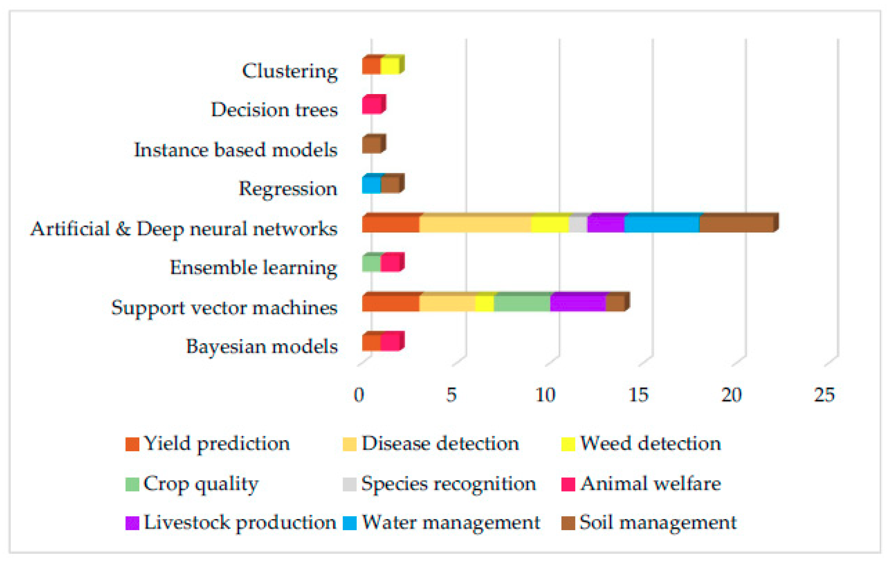
| ML Models Per Section | |||||||||
|---|---|---|---|---|---|---|---|---|---|
| Model | Crop | Livestock | Water | Soil | |||||
| Yield Prediction | Disease Detection | Weed Detection | Crop Quality | Species Recognition | Animal Welfare | Livestock Production | Water Management | Soil Management | |
| Bayesian models | 1 | 1 | |||||||
| Support vector machines | 3 | 3 | 1 | 3 | 3 | 1 | |||
| Ensemble learning | 1 | 1 | |||||||
| Artificial & Deep neural networks | 3 | 6 | 2 | 1 | 2 | 4 | 4 | ||
| Regression | 1 | 1 | |||||||
| Instance based models | 1 | ||||||||
| Decision trees | 1 | ||||||||
| Clustering | 1 | 1 | |||||||
| Total | 8 | 9 | 4 | 4 | 1 | 3 | 5 | 5 | 7 |
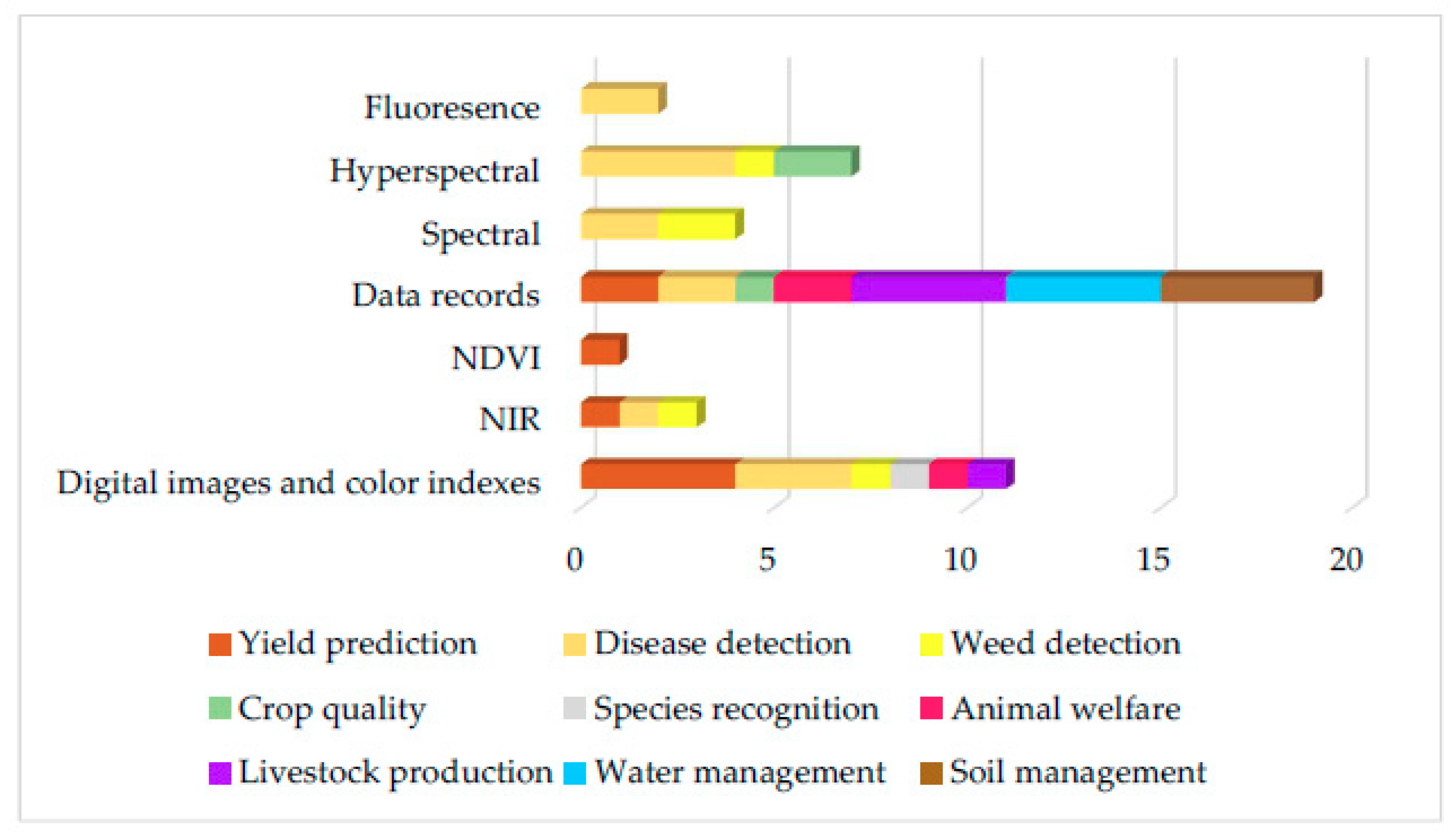
| Feature Collection | |||||||||
|---|---|---|---|---|---|---|---|---|---|
| Feature Technique | Crop | Livestock | Water | Soil | |||||
| Yield Prediction | Disease Detection | Weed Detection | Crop Quality | Species recognition | Animal Welfare | Livestock Production | Water Management | Soil Management | |
| Digital images and color indexes | 4 | 3 | 1 | 1 | 1 | 1 | |||
| NIR | 1 | 1 | 1 | ||||||
| NDVI | 1 | ||||||||
| Data records | 2 | 2 | 1 | 2 | 4 | 4 | 4 | ||
| Spectral | 2 | 2 | |||||||
| Hyperspectral | 4 | 1 | 2 | ||||||
| Fluoresence | 2 | ||||||||
© 2018 by the authors. Licensee MDPI, Basel, Switzerland. This article is an open access article distributed under the terms and conditions of the Creative Commons Attribution (CC BY) license (http://creativecommons.org/licenses/by/4.0/).
Share and Cite
Liakos, K.G.; Busato, P.; Moshou, D.; Pearson, S.; Bochtis, D. Machine Learning in Agriculture: A Review. Sensors 2018, 18, 2674. https://doi.org/10.3390/s18082674
Liakos KG, Busato P, Moshou D, Pearson S, Bochtis D. Machine Learning in Agriculture: A Review. Sensors. 2018; 18(8):2674. https://doi.org/10.3390/s18082674
Chicago/Turabian StyleLiakos, Konstantinos G., Patrizia Busato, Dimitrios Moshou, Simon Pearson, and Dionysis Bochtis. 2018. "Machine Learning in Agriculture: A Review" Sensors 18, no. 8: 2674. https://doi.org/10.3390/s18082674