Quantifying Invasive Pest Dynamics through Inference of a Two-Node Epidemic Network Model

Abstract

Invasive woodland pests have substantial ecological, economic, and social impacts, harming biodiversity and ecosystem services. Mathematical modelling informed by Bayesian inference can deepen our understanding of the fundamental behaviours of invasive pests and provide predictive tools for forecasting future spread. A key invasive pest of concern in the UK is the oak processionary moth (OPM). OPM was established in the UK in 2006; it is harmful to both oak trees and humans, and its infestation area is continually expanding. Here, we use a computational inference scheme to estimate the parameters for a two-node network epidemic model to describe the temporal dynamics of OPM in two geographically neighbouring parks (Bushy Park and Richmond Park, London). We show the applicability of such a network model to describing invasive pest dynamics and our results suggest that the infestation within Richmond Park has largely driven the infestation within Bushy Park.

1. Introduction

The spread of invasive pests, including non-native insects within urban treescapes, woodlands, and forests is having profound environmental, economic and social impacts [1,2,3]. In the UK, invasive species are estimated to have cost GBP 5–13 billion since 1976 through damages and management costs, and impacts on ecosystem services [4]. Thus, the UK government has identified enhancing biosecurity as a key priority, aiming to control existing pests and build resilience against emerging concerns by harnessing computational modelling methods [5].

Statistical and mathematical computational models can be used to explore the fundamental behaviours of pest infestations and facilitate quantitative predictions of the future spread. Commonly employed models include dynamical system models consisting of differential equations that describe pest population numbers and movements across landscapes, such as those for the grey squirrel in Wales [6]. Stochastic epidemic models [7] are more commonly used to describe disease dynamics within a population, but are transferable to the application of invasive pest spread [8]. In our previous work [9], we demonstrated that such an approach was indeed transferable to exploring invasive pest dynamics, and we build upon that framework here.

A key invasive pest of concern for treescapes within the UK and northern mainland Europe is the oak processionary moth (OPM), Thaumetopoea processionea (Linnaeus, 1758) (Lepidoptera: Notodontidae). OPM is a univoltine Lepidoptera that feeds on the Quercus species [10]. Female moths lay eggs in branches of the tree canopy in the summer, with larvae (caterpillars) emerging in the spring of the next year [11,12]. The larvae go through six instars, grouping together to form aggregates and constructing communal silk nests in the later instars [12]. The larvae pupate in the nests with adult moths emerging in mid-July [12,13]. Native to southern Europe, OPM was first established in the UK in 2006 through an accidental import.

OPM is destructive to oak trees, causing defoliation, which can leave infested trees vulnerable to other stressors [12]. Protecting the oak tree population is crucial for promoting biodiversity, with thousands of species known to be supported by the oak [14,15]. Additionally, OPM larvae have poisonous hairs, which contain a urticating toxin that is harmful to both human and animal health [16,17]. Despite great efforts to contain the UK infestation to the originally affected area of south-east England [17], the extent of OPM continues to spread, with an expansion rate estimated at 1.7 km/year for 2006–2014, with an increase to 6 km/year from 2015 onward [13]. There is evidence to suggest that the regions surrounding the current infestation area are particularly climatically suitable [18] and, thus, the prediction and control of the OPM population at its outer extent are especially crucial. Previous models for OPM have included species distribution models to predict future infestation under climate change [18] and electric network theory models to predict high-risk regions [19].

In our previous work [9], we considered the temporal population of OPM in two London parks (Bushy Park and Richmond Park), applying a novel Bayesian inference scheme to estimate the parameters for a compartmental epidemic model with a time varying infestation rate. This showed that the infestation rate in both parks remained relatively constant between 2013 and 2021, despite the control methods in place, resulting in the observed continual expansion of the infestation area [13].

In this paper, we build upon the work in [9], challenging the assumption that the infestations within the two parks are independent of each other, due to their neighbouring geographical locations. Thus, here we consider a two-node compartmental epidemic model, using analogous computational inference methods (making use of a linear Gaussian approximation to the stochastic susceptible-infected-removed (SIR) model and a Markov chain Monte Carlo scheme) to estimate the infestation parameters, including a quantification of each park’s influence upon its neighbour. The data, model, and inference scheme are detailed in Section 2, with the results presented in Section 3 and further discussion in Section 4. Our findings demonstrate the applicability of a two-node compartmental model to describe OPM spread and provide a framework applicable to other partially observed time series for infestations.

2. Materials and Methods

In this section, we present the observational OPM data (Section 2.1), detail the two-node SIR epidemic model (Section 2.2) and outline the statistical methods used to estimate the model parameters (Section 2.3 and Section 2.4).

2.1. The Data

We consider the OPM infestation within two London parks: Bushy Park and Richmond Park. The data consist of the numbers and locations (eastings and northings) of removed OPM nests between 2013 and 2021. The data are collected and processed by The Royal Parks and shared with the Forestry Commission to inform the national OPM Control Programme. The University of Southampton (GeoData) provides analyses and support, and holds the data on behalf of the Forestry Commission.

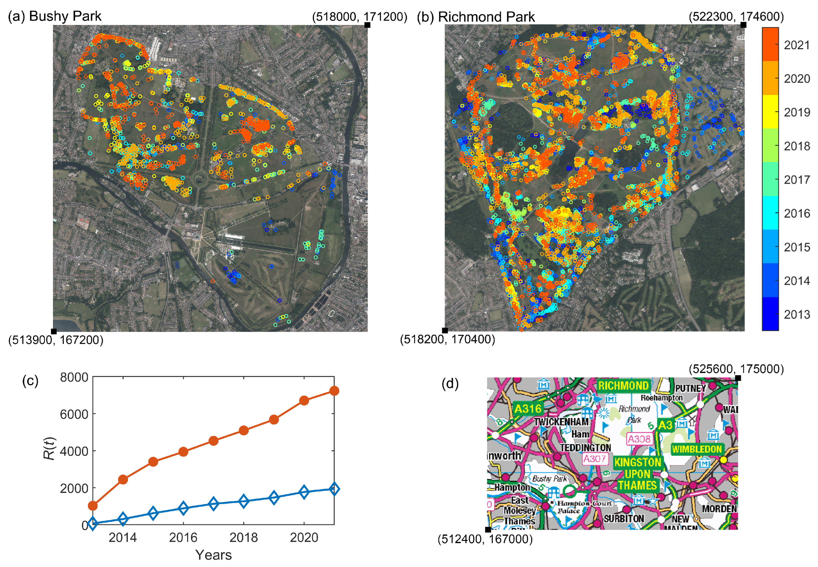
A summary of the OPM nest presence (and immediate removal) in both parks is shown in Figure 1a,b. We consider the cumulative time series of previously infested trees (those recorded as having nests removed) as our observed data in the following sections, shown in Figure 1c. This corresponds to the ‘Removed’ category prevalence in the compartmental SIR model presented in the next section, as in [9]. We refer to this as a partially observed dataset as we only have information about one of the categories in the compartmental SIR model. The neighbouring geographical location of the two parks, shown in Figure 1d, motivates our choice to consider a two-node epidemic network model, outlined in the next section.

2.2. The Two-Node Model

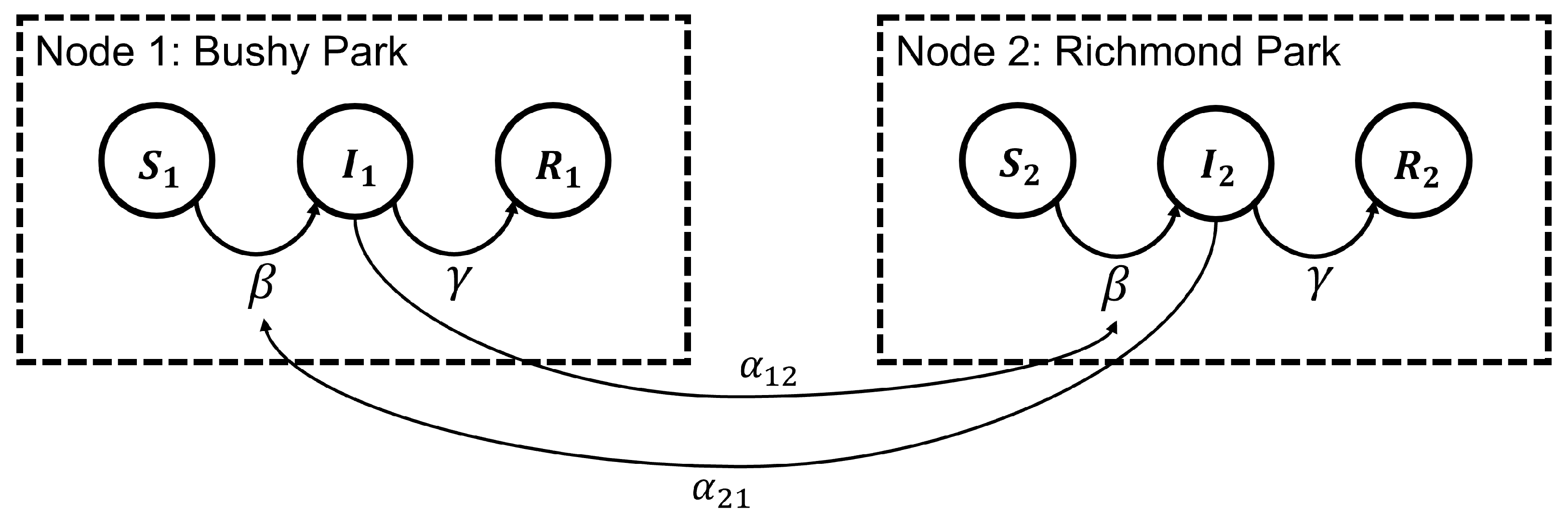
In [9], we applied a stochastic SIR epidemic model [22] to the spread of OPM in Bushy Park and Richmond Park between 2013 and 2021. Here, we expand this model, noting that the two parks are close in geographical location, as shown in Figure 1d and, thus, the OPM dynamics within each park may not be independent of each other. We therefore consider a similar stochastic SIR model but for two connected nodes (here representing each of the two parks) as illustrated in Figure 2. Further mathematical details of the stochastic SIR epidemic model can be found in [22,23], with details of its formulation as a discrete-valued Markov jump process (MJP) in [24].

Within each node, the fixed population of the tree transition between the compartmental states: S, susceptible (not yet infested), I, infested (currently infested), and R removed (no longer infested or contributing to the infestation spread). The transition between the infested and removed state is governed by the removal rate parameter, $\gamma$. The transition between the S and I compartments is governed not only by the standard infestation rate parameter $\beta$ (the rate at which contact of one infested tree with one susceptible tree will result in infestation, referred to as the ‘effective contact rate’), but also an additional infestation ‘pressure’ from the neighbouring node, described by the parameters ${\alpha }_{ij}$, where ${\alpha }_{12}$ is the pressure applied by node 1 on node 2, and ${\alpha }_{21}$ the pressure from node 2 on node 1. A similar model has been previously proposed to describe national surveillance counts from the 2013 to 2015 West Africa Ebola outbreak [25].

We assume that the effective contact rate $\beta$ and the removal rate $\gamma$ are the same in both parks as parameters inherent to the OPM population under similar conditions. The effective contact rate $\beta$ can be expressed as $\beta =\kappa \tau /N$, where $\kappa$ is the number of contacts (opportunities for transmission) and $\tau$ is the transmissibility of the disease (here, the pest). Since $\tau$ is inherent to the system, the assumption of equal effective contact rates in each node results in ${\kappa }_1/N_1={\kappa }_2/N_2$ and, thus, a number of contacts $\kappa$ that is proportional to the population size within each node.

The dynamics of all compartment states in the two-node model above are most naturally described by a MJP, whereby state numbers are described via a continuous-time Markov process with a discrete state space, reflecting the fact that states change abruptly and discretely in time [7]. As noted in [26], this can be computationally prohibitive for models in which typical population sizes are more than a few hundred. Therefore, we eschew the MJP representation in favour of a tractable continuous approximation via a stochastic differential equation (SDE). We describe the SDE below before considering a further tractable approximation known in the stochastic kinetics literature as the linear noise approximation (LNA). We refer the reader to [27] for further details on the SDE and LNA approximation of an MJP.

The corresponding stochastic differential equation model considers the latent process $X_t={(S_{1,t},I_{1,t},S_{2,t},I_{2,t})}^{\prime }$, where $S_{i,t}$ and $I_{i,t}$ denote the number of trees in each of the compartments S and I in node i at time $t\ge 0$. The complete SDE model can be described by

$$d{X}_t=a(x_t,\theta )dt+\sqrt{b(x_t,\theta )}d{W}_t,$$

(1)

where $x_t=(s_{1,t},i_{1,t},s_{2,t},i_{2,t})$ is the state of the system at time t, $\theta ={(\beta ,\gamma ,{\alpha }_{12},{\alpha }_{21})}^{\prime }$ is the vector of parameter values and $d{W}_t={(W_{1,t},W_{2,t},W_{3,t},W_{4,t})}^{\prime }$ denotes uncorrelated standard Brownian motion processes on each of the compartmental states. The SDE drift function $a(x_t,\theta )$ and diffusion coefficient $b(x_t,\theta )$ are given by

$$a(x_t,\theta )=\left(\begin{array}{c}-\beta (i_{1,t}+{\alpha }_{21}{i}_{2,t})s_{1,t}\\ \beta (i_{1,t}+{\alpha }_{21}{i}_{2,t})s_{1,t}-\gamma i_{1,t}\\ -\beta (i_{2,t}+{\alpha }_{12}{i}_{1,t})s_{2,t}\\ \beta (i_{2,t}+{\alpha }_{12}{i}_{1,t})s_{2,t}-\gamma i_{2,t}\end{array}\right),$$

(2)

and

$$b(x_t,\theta )=\left(\begin{array}{cc}{b}_{11}& 0_{2,2}\\ 0_{2,2}& b_{22}\end{array}\right),$$

(3)

where

$$b_{11}=\left(\begin{array}{cc}\beta (I_{1,t}+{\alpha }_{21}{I}_{2,t})S_{1,t}& -\beta (I_{1,t}+{\alpha }_{21}{I}_{2,t})S_{1,t}\\ -\beta (I_{1,t}+{\alpha }_{21}{I}_{2,t})S_{1,t}& \beta (I_{1,t}+{\alpha }_{21}{I}_{2,t})S_{1,t}+\gamma I_{1,t}\end{array}\right),$$

(4)

and

$$b_{22}=\left(\begin{array}{cc}\beta (I_{2,t}+{\alpha }_{12}{I}_{1,t})S_{2,t}& -\beta (I_{2,t}+{\alpha }_{12}{I}_{1,t})S_{2,t}\\ -\beta (I_{2,t}+{\alpha }_{12}{I}_{1,t})S_{2,t}& \beta (I_{2,t}+{\alpha }_{12}{I}_{1,t})S_{2,t}+\gamma I_{2,t}\end{array}\right),$$

(5)

and $0_{2,2}$ is the $2\times 2$ zero matrix. Since the SDE specified by (1)–(5) cannot be solved analytically, we replace the intractable analytic solution with a tractable Gaussian process approximation: the LNA, described in the next section.

2.3. Linear Noise Approximation

The LNA provides a tractable approximation to the SDE given in (1)–(5). We used the LNA in the same manner for a stochastic SIR model with a time-varying infestation rate, also applied to OPM, in [9]. Formal details of the LNA can be found in [28,29,30]; below we outline the derivation.

Consider a partition of $X_t$ as

$$X_t={\eta }_t+Z_t,$$

(6)

where $\{{\eta }_t,t\ge 0\}$ is a deterministic process satisfying the ordinary differential equation (ODE)

$$\frac{d{\eta }_t}{dt}=a({\eta }_t,\theta ),{\eta }_0=x_0,$$

(7)

and $\{Z_t,t\ge 0\}$ is a residual stochastic process. The residual process $Z_t$ satisfies

$$d{Z}_t=\{a(x_t,\theta )-a({\eta }_t,\theta )\}dt+\sqrt{b(x_t,\theta )}d{W}_t,$$

which will typically be intractable. The assumption that $\left|\right|X_t-{\eta }_t\left|\right|$ is “small” motivates a Taylor series expansion of $a(x_t,\theta )$ and $b(x_t,\theta )$ about ${\eta }_t$, with retention of the first two terms in the expansion of a and the first term in the expansion of b. This gives an approximate residual process $\{{\widehat{Z}}_t,t\ge 0\}$ satisfying

$$d{\widehat{Z}}_t=H_t{\widehat{z}}_{t}dt+\sqrt{b({\eta }_t,\theta )}d{W}_t,$$

where $H_t$ is the Jacobian matrix with (i,j)th element

$${\left(H_t\right)}_{i,j}=\frac{\partial a_i({\eta }_t,\theta )}{\partial {\eta }_{j,t}}.$$

Therefore, for the SIR model in (1)–(5) we have

$$H_t=\left(\begin{array}{cccc}-\beta (i_{1,t}+{\alpha }_{21}{i}_{2,t})& -\beta s_{1,t}& 0& -\beta {\alpha }_{21}{s}_{1,t}\\ \beta (i_{1,t}+a_{21}{i}_{2,t})& \beta s_{1,t}-\gamma & 0& \beta {\alpha }_{21}{s}_{1,t}\\ 0& -\beta a_{12}{s}_{2,t}& -\beta (i_{2,t}+a_{12}{i}_{1,t})& -\beta s_{2,t}\\ 0& \beta a_{12}{s}_{2,t}& \beta (i_{2,t}+a_{12}{i}_{1,t})s_{2,t}& \beta s_{2,t}-\gamma \end{array}\right).$$

Given an initial condition ${\widehat{Z}}_0\sim \mathrm{N}({\widehat{z}}_0,{\widehat{V}}_0)$, it can be shown that ${\widehat{Z}}_t$ is a Gaussian random variable [31]. Consequently, the partition in (6) with $Z_t$ replaced by ${\widehat{Z}}_t$, and the initial conditions ${\eta }_0=x_0$ and ${\widehat{Z}}_0=0$ give

$$X_t\sim \mathrm{N}\left({\eta }_t,V_t\right),$$

(8)

where ${\eta }_t$ satisfies (7) and $V_t$ satisfies

$$\frac{d{V}_t}{dt}=V_t{H}_t^{\prime }+b({\eta }_t,\theta )+H_t{V}_t,V_0=0.$$

(9)

Further details on the derivation of (9) are given in [9]. Hence, the linear noise approximation is characterised by the Gaussian distribution in (8), with mean and variance found by solving the ODE system given by (7) and (9), which can be solved numerically.

2.4. Bayesian Inference

We consider the case in which not all components of the stochastic epidemic model are observed and that the data points are subject to measurement error, as in [9]. Observations (on a regular grid) $y_t,t=0,1,\dots n$ are assumed conditionally independent (given the latent process $X_t$) with conditional probability distribution obtained via the observation equation,

$$Y_t\sim \mathrm{N}\left(P{x}_t,{\sigma }^2\mathrm{diag}\left\{P{x}_t\right\}\right),t=0,1,\dots ,n$$

(10)

where

$$P=\left(\begin{array}{cccc}1& 1& 0& 0\\ 0& 0& 1& 1\end{array}\right).$$

(11)

This choice of P is due to the data consisting of observations on the removed states in each node, $R_{1,t}$ and $R_{2,t}$, which for known population sizes $N_1$ and $N_2$, is equivalent to observing the sums $S_{1,t}+I_{1,t}$ and $S_{2,t}+I_{2,t}$. Our choice of observation model is motivated by a Gaussian approximation of two independent Poisson random variables with rates given by the components of $P{x}_t$. Moreover, the assumption of a Gaussian observation model admits a tractable observed data likelihood function, when combined with the LNA (see Section 2.3 and [31,32]) as a model for the latent epidemic process $X_t$. Details on a method for the efficient evaluation of this likelihood function can be found in [9].

Given data $y=(y_0,y_1,\dots ,y_n)$ and upon ascribing a prior density $\pi \left(\theta \right)$ to the components of $\theta ={(\beta ,\gamma ,{\alpha }_{12},{\alpha }_{21},\sigma )}^{\prime }$, Bayesian inference proceeds via the joint posterior for the static parameters $\theta$ and unobserved dynamic process $x=(x_0,x_1,\dots ,x_n)$. We have that

$$\pi (\theta ,x|y)\propto \pi (\theta \left)\pi \right(y\left|\theta \right)\pi \left(x\right|y,\theta ),$$

(12)

where $\pi \left(y\right|\theta )$ is the observed data likelihood and $\pi \left(x\right|y,\theta )$ is the conditional posterior density of the latent dynamic process. We use a Markov chain Monte Carlo scheme for generating (dependent) samples from (12) due to the intractable joint posterior. Briefly, this comprises two steps: i) the generation of samples ${\theta }^{\left(1\right)},\dots ,{\theta }^{\left(M\right)}$ from the marginal parameter posterior $\pi \left(\theta \right|y)\propto \pi (\theta \left)\pi \right(y\left|\theta \right)$ and ii) the generation of samples $x^{\left(1\right)},\dots ,x^{\left(M\right)}$ by drawing from the conditional posterior $\pi \left(x\right|y,{\theta }^{\left(i\right)})$, $i=1,\dots ,M$.

The parameters required as input for the inference scheme are given in

Table 1. The input parameters used in the inference scheme for the two-node model detailed in Section 2.2, Section 2.3 and Section 2.4.

Input Parameters
Total population	$N_1=5000$, $N_2$ = 40,000
Initial infested	$I_{1,0}=240$, $I_{2,0}=1400$
Initial model parameters	${\theta }_0=({\beta }_0,{\gamma }_0,{\alpha }_{{12}_0},{\alpha }_{{21}_0},{\sigma }_0)=(0.00001,0.8,0.3,2.5,1)$
Prior distributions	$log{\theta }_i\sim$N(0, 1${}^2$),    $i=1,\dots ,4$
Tuning parameter	$\Sigma =\left(\begin{array}{ccccc}0.009& 0.003& -0.059& -0.009& 0.002\\ 0.003& 0.006& 0.011& 0.001& 0.001\\ -0.059& 0.011& 0.712& 0.072& -0.006\\ -0.009& 0.001& 0.072& 0.013& -0.002\\ 0.002& 0.001& -0.006& -0.002& 0.052\end{array}\right)$
Initial ODE mean	$x_0={\eta }_0=(N_1-I_{1,0}-R_{1,0},I_{1,0},N_2-I_{2,0}-R_{2,0},I_{2,0})$
Initial ODE variance	$V_0=0_{4,4}$
Observation matrix	$P=\left(\begin{array}{cccc}1& 1& 0& 0\\ 0& 0& 1& 1\end{array}\right)$

. We take estimates of the number of trees in each park and the infestation initial conditions as in [9], with $N_1=5000$ (Bushy) and $N_2=40,000$ (Richmond) and initial ODE conditions $x_0=(S_{1,0},I_{1,0},S_{2,0},I_{2,0})=(N_1-I_{1,0}-R_{1,0},I_{1,0},N_2-I_{2,0}-R_{2,0},I_{2,0})$.

The methodology described above overcomes the challenge of the data being partially observed and handles a relatively short observed time series (in this case, nine data points). This is transferable to other epidemic datasets. If the data considered is more limited, this could result in larger uncertainties in the plausible ranges of the estimated parameters.

3. Results

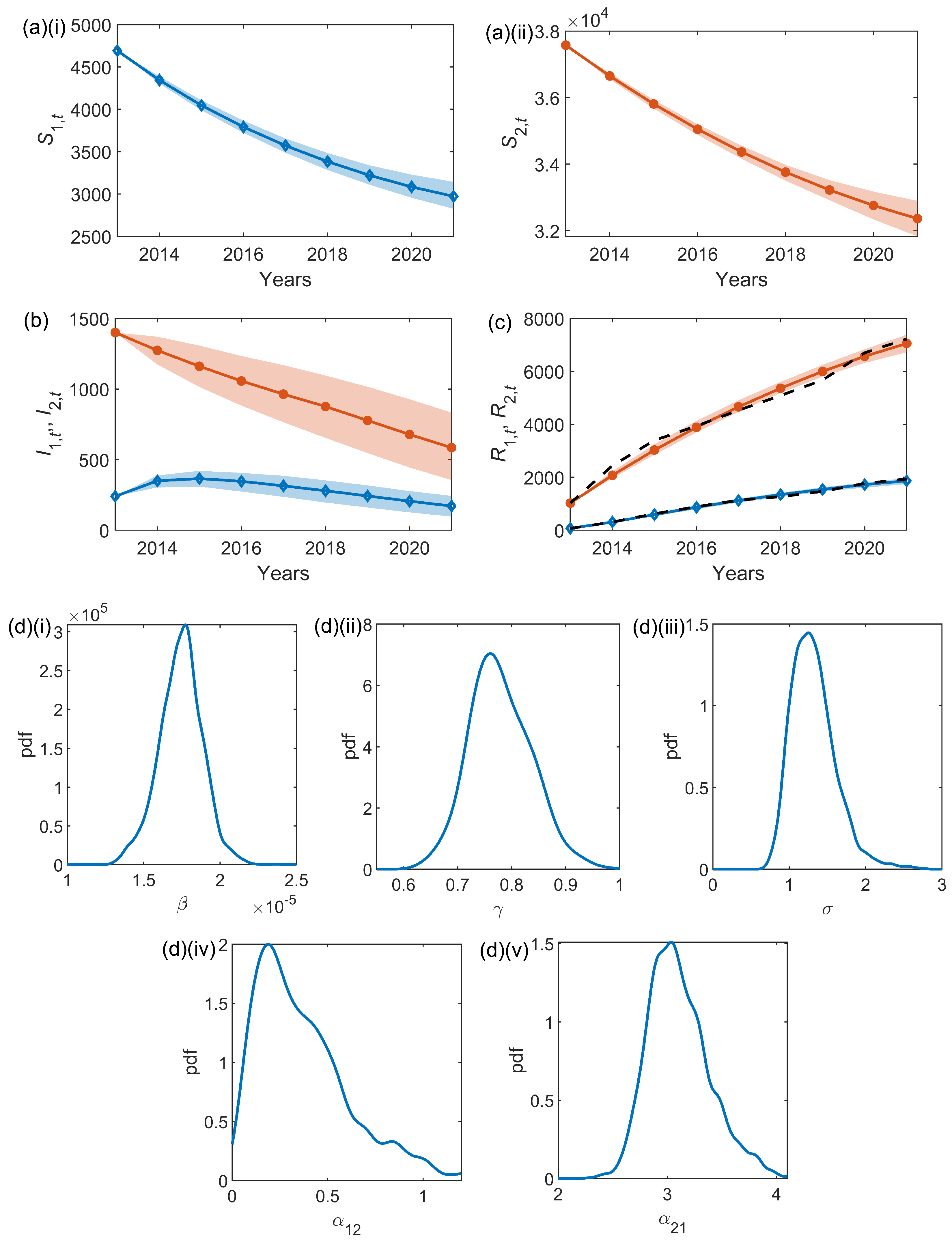
We take the data, detailed in Section 2.1 and pictured in Figure 1, for the cumulative number of trees with removed OPM nests in Bushy Park and Richmond Park. We (arbitrarily) denote Bushy Park as node 1, and Richmond Park as node 2, with the observed data corresponding to the removal prevalence time series $R_{1,t}$ and $R_{2,t}$ in the two-node model described in Section 2.2. Through the inference techniques outlined in Section 2.3 and Section 2.4, we infer the parameters for the two-node stochastic epidemic model: the infestation rate $\beta$, and removal rate $\gamma$, common to both nodes, along with additional parameters representing the infestation ‘pressure’ resulting from the neighbouring node, ${\alpha }_{12}$ and ${\alpha }_{21}$, and an observation error $\sigma$.

The results from the inference scheme are shown in Figure 3 with within-sample median posterior series for $S_{i,t}$, $I_{i,t}$ and $R_{i,t}$, and posterior densities of the inferred parameters. The average parameter results are shown in full in

Table 2. The posterior means, standard deviations, medians, and 95% credible intervals for the inferred model parameters.

Parameter	Mean	Standard Deviation	Median	95% Credible Interval
$\beta$	$1.74\times {10}^{-5}$	$1.40\times {10}^{-6}$	$1.75\times {10}^{-5}$	$(1.44,2.02)\times {10}^{-5}$
$\gamma$	$0.78$	$0.056$	$0.77$	$(0.67,0.90)$
$\sigma$	$1.32$	$0.289$	$1.28$	$(0.88,1.99)$
${\alpha }_{12}$	$0.38$	$0.268$	$0.32$	$(0.06,1.05)$
${\alpha }_{21}$	$3.12$	$0.312$	$3.08$	$(2.66,3.83)$

. The median infestation rate is $\beta \approx 1.8\times {10}^{-5}$, the median removal rate is $\gamma \approx 0.8$, and the median observation error (see (10)) is $\sigma \approx 1.3$. The median posterior estimates of the parameters connecting the two nodes are ${\alpha }_{12}\approx 0.3$ (Bushy to Richmond) and ${\alpha }_{21}\approx 3$ (Richmond to Bushy).

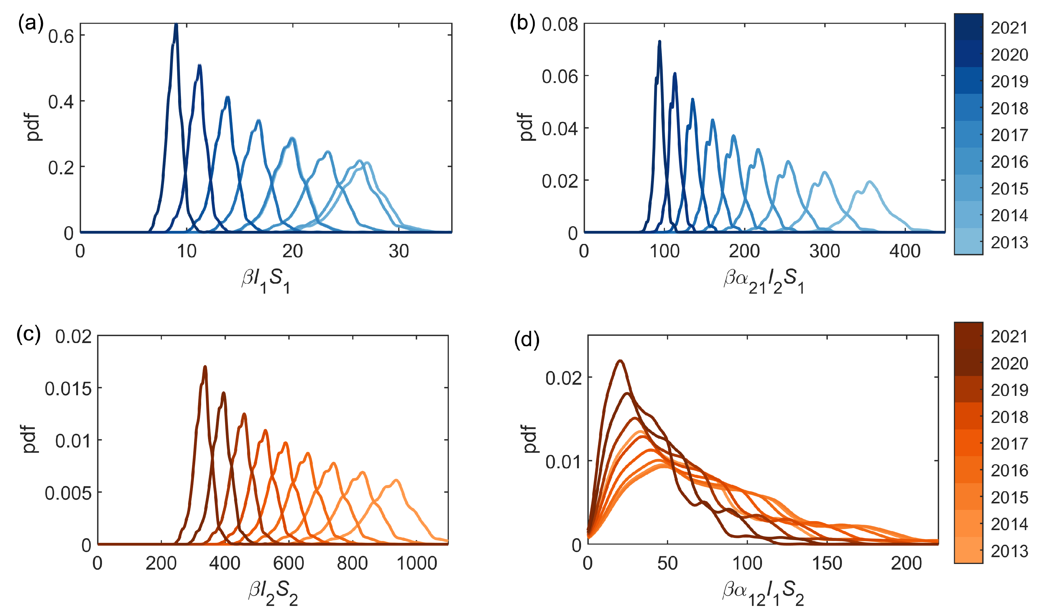
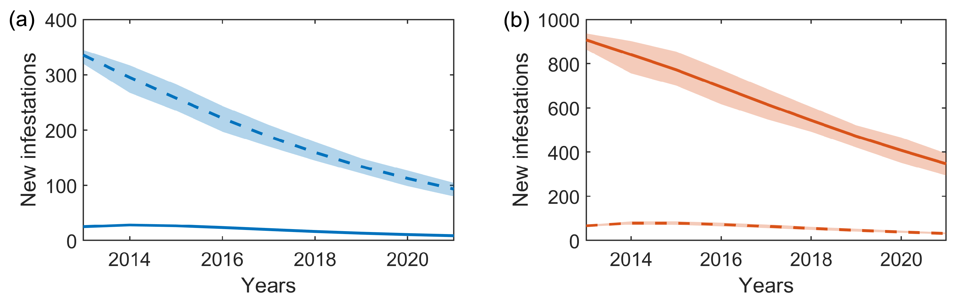
We can consider each of the infestation components (see (2)): the standard intra-park component $\beta I_i{S}_i$, and the connecting inter-park component $\beta {\alpha }_{ij}{I}_i{S}_j$. Probability densities for both the intra- and inter-park infestation components using the median posterior estimates of $S_{i,t}$ and $I_{i,t}$, and the full posterior distributions of $\beta$ and ${\alpha }_{ij}$, are shown in Figure 4. Similarly, the expected number of new infestations from each of the two components, averaged over 50 forward simulations with the median parameters estimated through the inference scheme (Table 2), are shown in Figure 5. Both Figure 4 and Figure 5 illustrate that in Bushy Park the inter-park dynamics (Richmond–Bushy) are significantly greater than the intra-park (Bushy–Bushy), whereas in Richmond Park the intra-park dynamics (Richmond–Richmond) are more significant than the inter-park (Bushy-Richmond). This suggests that the infestation in Bushy Park has been largely driven by the infestation in Richmond Park to a greater extent than vice versa.

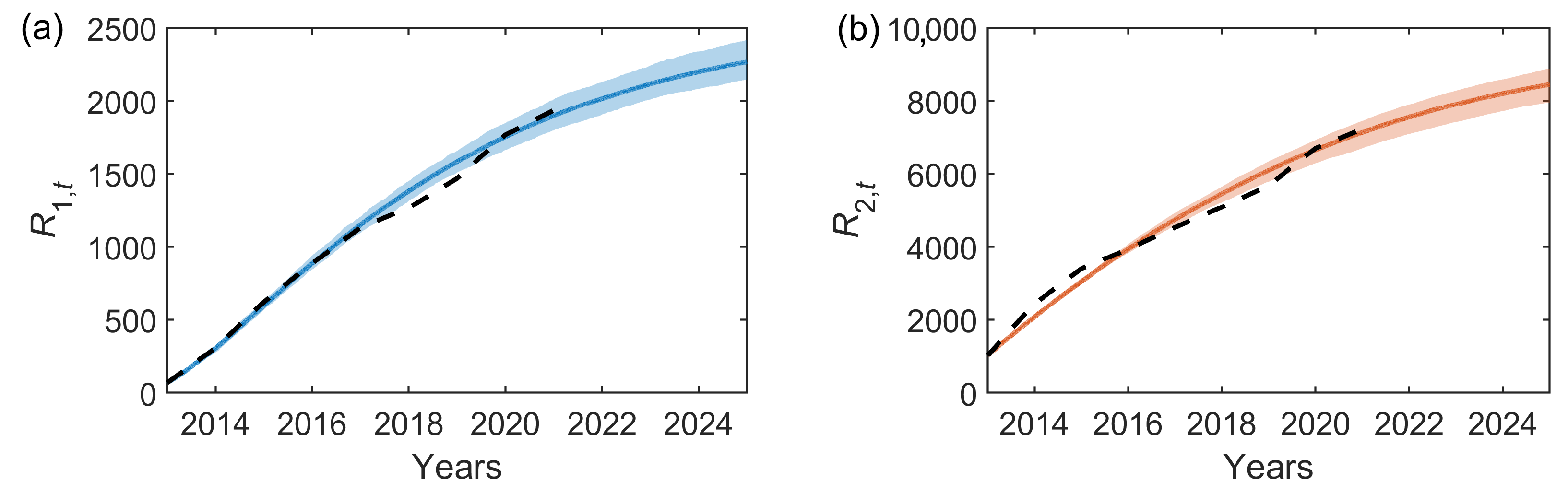
Predictions of the spread of OPM are required to inform management strategies. We can use the inferred model parameters to simulate the infestation forwards in time. The simulated removal prevalence time series resulting from the stochastic two-node epidemic model with the median inferred parameter estimates is shown in Figure 6 for the years 2013 to 2025. Here, we see the overall alignment with the observational data, with a deviation between 2017 and 2020 in which the infestation numbers were lower than this model predicts, and the future forecasting if the infestation were to continue with these characteristic parameters.

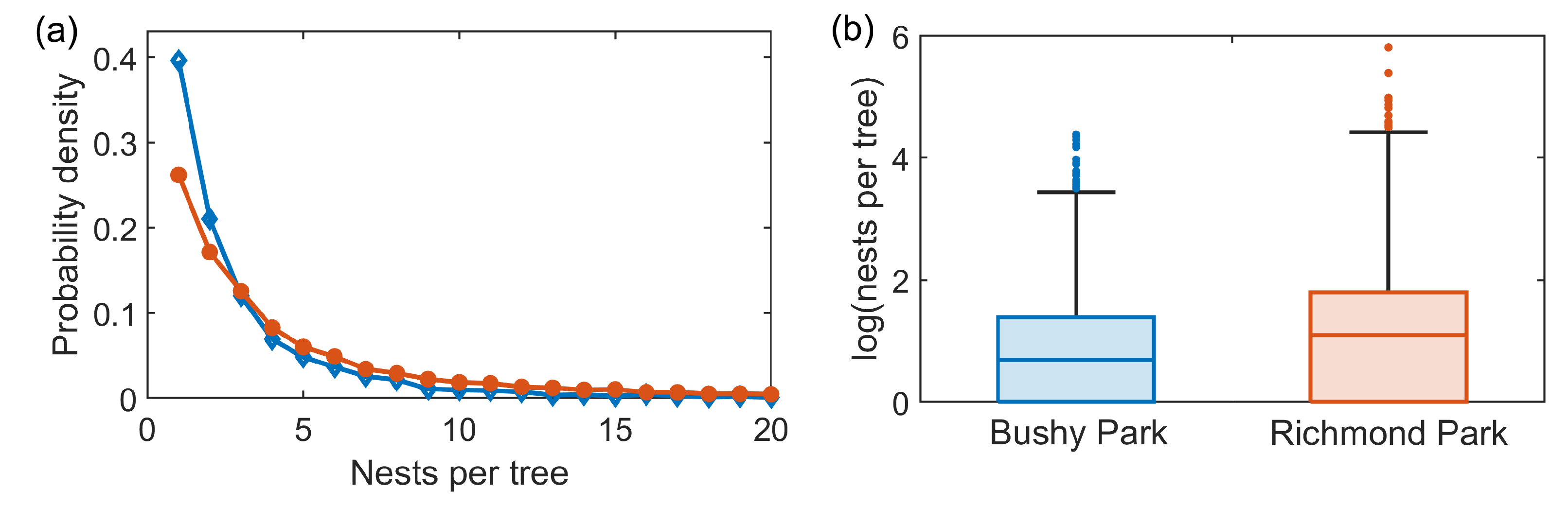
A possible contributing factor to the dynamics, not considered explicitly in this epidemic model, is the density of OPM nests within each park, i.e., the number of nests per infested tree, shown in Figure 7. Richmond park has a slightly higher infestation density, with a median of three nests per infested tree, compared to the median of two nests per tree in Bushy Park, and an upper quartile of six nests per tree, compared to the upper quartile of four in Bushy Park. This increased nest density could contribute to the resulting infestation pressure from the Richmond Park infestation to the Bushy Park infestation.

4. Discussion

It is crucial to deepen our understanding of the dynamics of invasive pests to develop predictive modelling tools and maximise the impact of control strategies. Here, we show the applicability of two-node compartmental epidemic models, using case study data of the OPM infestations within the neighbouring Bushy Park and Richmond Park in London.

In our previous work exploring the UK OPM infestation [9], we considered the two parks as independent contained areas and estimated the parameters for a compartmental model with a time-varying infestation rate, showing the infestation rate had remained stable over time. Here we challenge the assumption that the infestations within the two parks are independent due to their geographical proximity (with the closest park boundaries separated by approximately 2–3 km).

Instead, we assume that the infestation contact rate within each park, $\beta$, (assumed to be a constant based on the results from [9]) and the removal rate, $\gamma$, are inherent properties of the OPM species under similar conditions, resulting in identical $\beta$ and $\gamma$ in both nodes (parks). Since $\beta$ can be expressed as $\kappa \tau /N$, with $\kappa$ the number of contacts and $\tau$ a transmissibility parameter inherent to the species, we have ${\kappa }_1/N_1={\kappa }_2/N_2$ and, thus, the number of contacts scales with the total population number. In the case of OPM, this corresponds to an increasing number of ‘contacts’ between trees due to the underlying movement of the OPM population, an assumption that would hold whilst the typical movement distances of OPM are of a similar (or greater) length scale to the tree population area, i.e., a greater number of trees (increased N) means a greater number of opportunities for contacts (increased $\kappa$) providing the moths can travel over the whole area. Despite the joint infestation parameters $\beta$ and $\gamma$, the infestation dynamics can still differ in each park due to different numbers of susceptible trees and the introduction of two additional parameters connecting the infestations within the two nodes, ${\alpha }_{12}$ and ${\alpha }_{21}$.

Similar epidemic models have previously been used to describe the spread of infectious disease within human populations, e.g., for Ebola in [25]. In these cases, the parameters connecting the nodes represent the rates of the movement of individuals between nodes, e.g., the movement of infected people between geographical locations. In the case of our OPM model, the individuals within each of the SIR compartments are trees, which are spatially fixed and, thus, ${\alpha }_{ij}$ instead represents a proxy measure of the movement of the underlying OPM population between the two nodes. The movement patterns of OPM are not fully characterised, but can occur through three possible routes: short-distance larvae movement, flight of adult moths, and accidental human-mediated dispersal [13,33]. Considering the locations of the two parks considered here, the latter two dispersal mechanisms are possibilities for facilitating moth movement between nodes.

We find that the connecting parameter representing the infestation pressure on the trees in Bushy Park resulting from the infestation in Richmond park is much stronger than vice versa. The infestation in Richmond Park is relatively unaffected by the infestation in Bushy Park. One reason for the observed Richmond-led infestation dynamics could be the higher underlying nest density within the park, resulting in a greater population density of OPM per susceptible tree, a larger contact number, $\kappa$, and more opportunities for longer-range movement between the two parks. The relationships between OPM nest density, tree height, infestation percentages, and bacterial control treatment are explored in [34].

We note that there are control measures taking place in many OPM-infested areas [35]. In Bushy and Richmond Parks, control measures include the yearly nest removal (leading to the data used here) and limited spraying with a biological insecticide which has been shown to reduce nest density [34]. Thus, all inferred parameters represent the infestation dynamics under these conditions, rather than inherent parameters of uncontrolled pest spread. Although not ideal for learning about the fundamental properties of the species, this is necessary as emergent invasive pests require an immediate control response.

Future work could explore expanding the epidemic network to a greater number of areas (nodes), forming more connections across the wider OPM-infested area of south-east England. If a similar approach to network building was taken to that described in [19], the results from the statistical compartmental epidemic model could be compared with the electric network theory model [19]. However, expanding the network represents a computational challenge, with increasing numbers of parameters to infer.

The results from this work can inform the development of future computational models for the spread of OPM, and provide a statistical framework for applying to other emerging pest concerns with similar partially-observed temporal data sets.

References

- Manchester, S.J.; Bullock, J.M. The impacts of non-native species on UK biodiversity and the effectiveness of control. J. Appl. Ecol. 2000, 37, 845–864. [Google Scholar] [CrossRef]
- Kenis, M.; Auger-Rozenberg, M.; Roques, A.; Timms, L.; Péré, C.; Cock, M.J.W.; Settele, J.; Augustin, S.; Lopez-Vaamonde, C. Ecological effects of invasive alien insects. Biol. Invasions 2009, 11, 21–45. [Google Scholar] [CrossRef]
- Freer-Smith, P.H.; Webber, J.F. Tree pests and diseases: The threat to biodiversity and the delivery of ecosystem services. Biodivers. Conserv. 2017, 26, 3167–3181. [Google Scholar] [CrossRef]
- Cuthbert, R.N.; Bartlett, A.C.; Turbelin, A.J.; Haubrock, P.J.; Diagne, C.; Pattison, Z.; Courchamp, F.; Catford, J.A. Economic costs of biological invasions in the United Kingdom. NeoBiota 2021, 67, 299–328. [Google Scholar] [CrossRef]
- Department for Environment Food Rural Affairs. A Plant Biosecurity Strategy for Great Britain; Department for Environment Food Rural Affairs: London, UK, 2021.
- Eiswerth, M.E.; Johnson, W.S. Managing nonindigenous invasive species: Insights from dynamic analysis. Environ. Resour. Econ. 2002, 23, 319–342. [Google Scholar] [CrossRef]
- Allen, L.J.S. A primer on stochastic epidemic models: Formulation, numerical simulation, and analysis. Infect. Dis. Model. 2017, 2, 128–142. [Google Scholar] [CrossRef]
- Hulme, P.E.; Baker, R.; Freckleton, R.; Hails, R.S.; Hartley, M.; Harwood, J.; Marion, G.; Smith, G.C.; Williamson, M. The Epidemiological Framework for Biological Invasions (EFBI): An interdisciplinary foundation for the assessment of biosecurity threats. NeoBiota 2020, 62, 161–192. [Google Scholar] [CrossRef]
- Wadkin, L.E.; Branson, J.; Hoppit, A.; Parker, N.G.; Golightly, A.; Baggaley, A.W. Inference for epidemic models with time-varying infection rates: Tracking the dynamics of oak processionary moth in the UK. Ecol. Evol. 2022, 12, e8871. [Google Scholar] [CrossRef]
- Wagenhoff, E.; Blum, R.; Engel, K.; Veit, H.; Delb, H. Temporal synchrony of Thaumetopoea processionea egg hatch and Quercus robur budburst. J. Pest Sci. 2013, 86, 193–202. [Google Scholar] [CrossRef]
- Groenen, F.; Meurisse, N. Historical distribution of the oak processionary moth Thaumetopoea processionea in Europe suggests recolonization instead of expansion. Agric. For. Entomol. 2012, 14, 147–155. [Google Scholar] [CrossRef]
- Wagenhoff, E.; Veit, H. Five years of continuous Thaumetopoea processionea monitoring: Tracing population dynamics in an arable landscape of South-Western Germany. Gesunde Pflanz. 2011, 63, 51–61. [Google Scholar] [CrossRef]
- Suprunenko, Y.F.; Castle, M.D.; Webb, C.R.; Branson, J.; Hoppit, A.; Gilligan, C.A. Estimating expansion of the range of oak processionary moth (thaumetopoea processionea) in the UK from 2006 to 2019. Agric. For. Entomol. 2021, 24, 53–62. [Google Scholar] [CrossRef]
- Mitchell, R.; Bellamy, P.; Ellis, C.; Hewison, R.; Hodgetts, N.; Iason, G.; Littlewood, N.; Newey, S.; Stockan, J.; Taylor, A. Collapsing foundations: The ecology of the British oak, implications of its decline and mitigation options. Biol. Conserv. 2019, 233, 316–327. [Google Scholar] [CrossRef]
- Mitchell, R.; Bellamy, P.; Ellis, C.; Hewison, R.; Hodgetts, N.; Iason, G.; Littlewood, N.; Newey, S.; Stockan, J.; Taylor, A. OakEcol: A database of Oak-associated biodiversity within the UK. Data Brief 2019, 25, 104120. [Google Scholar] [CrossRef] [PubMed]
- Mindlin, M.J.; Le Polain de Waroux, O.; Case, S.; Walsh, B. The arrival of oak processionary moth, a novel cause of itchy dermatitis, in the UK: Experience, lessons and recommendations. Public Health 2012, 126, 778–781. [Google Scholar] [CrossRef] [PubMed]
- Tomlinson, I.; Potter, C.; Bayliss, H. Managing tree pests and diseases in urban settings: The case of Oak Processionary Moth in London, 2006–2012. Urban For. Urban Green. 2015, 14, 286–292. [Google Scholar] [CrossRef] [Green Version]
- Godefroid, M.; Meurisse, N.; Groenen, F.; Kerdelhué, C.; Rossi, J.P. Current and future distribution of the invasive oak processionary moth. Biol. Invasions 2020, 22, 523–534. [Google Scholar] [CrossRef]
- Cowley, D.J.; Johnson, O.; Pocock, M.J.O. Using electric network theory to model the spread of oak processionary moth, Thaumetopoea processionea, in urban woodland patches. Landsc. Ecol. 2015, 30, 905–918. [Google Scholar] [CrossRef] [Green Version]
- Edina Digimap. High Resolution (25 cm) Vertical Aerial Imagery [JPG Geospatial Data], Scale 1:500. Available online: https://digimap.edina.ac.uk (accessed on 12 May 2022).
- Ordnance Survey. 1:250000 Scale Colour Raster™. 2021. Available online: https://osdatahub.os.uk/downloads/open (accessed on 21 September 2022).
- Kermack, W.O.; McKendrick, A.G. A contribution to the mathematical theory of epidemics. Proc. Maths. Phys. 1927, 115, 700–721. [Google Scholar]
- Andersson, H.K.; Britton, T. Stochastic Epidemic Models and Their Statistical Analysis; Lecture Notes in Statistics; Springer: New York, NY, USA, 2000; pp. 11–18. [Google Scholar]
- Ho, L.S.T.; Xu, J.; Crawford, F.W.; Minin, V.N.; Suchard, M.A. Birth/birth-death processes and their computable transition probabilities with biological applications. J. Math. Biol. 2018, 76, 911–944. [Google Scholar] [CrossRef]
- Fintzi, J.; Wakefield, J.; Minin, V.N. A linear noise approximation for stochastic epidemic models fit to partially observed incidence counts. Biometrics 2021, 78, 1530–1541. [Google Scholar] [CrossRef] [PubMed]
- Golightly, A.; Wilkinson, D.J. Bayesian parameter inference for stochastic biochemical network models using particle Markov chain Monte Carlo. Interface Focus 2011, 1, 807–820. [Google Scholar] [CrossRef] [PubMed] [Green Version]
- Fuchs, C. Inference for Diffusion Processes: With Applications in Life Sciences; Springer Science & Business Media: Berlin/Heidelberg, Germany, 2013. [Google Scholar]
- Kurtz, T.G. The relationship between stochastic and deterministic models for chemical reactions. J. Chem. Phys. 1972, 57, 2976–2978. [Google Scholar] [CrossRef]
- van Kampen, N.G. Stochastic Processes in Physics and Chemistry; North-Holland Personal Library; Elsevier: Amsterdam, The Netherlands, 2001. [Google Scholar]
- Komorowski, M.; Finkenstadt, B.; Harper, C.; Rand, D. Bayesian inference of biochemical kinetic parameters using the linear noise approximation. BMC Bioinform. 2009, 10, 343. [Google Scholar] [CrossRef] [Green Version]
- Fearnhead, P.; Giagos, V.; Sherlock, C. Inference for reaction networks using the Linear Noise Approximation. Biometrics 2014, 70, 457–466. [Google Scholar] [CrossRef] [Green Version]
- Golightly, A.; Henderson, D.A.; Sherlock, C. Delayed acceptance particle MCMC for exact inference in stochastic kinetic models. Stat. Comput. 2015, 25, 1039–1055. [Google Scholar] [CrossRef] [Green Version]
- Townsend, M. Oak processionary moth in the United Kingdom. Outlooks Pest Manag. 2013, 24, 32–38. [Google Scholar] [CrossRef]
- Straw, N.A.; Forster, J. The effectiveness of ground-based applications of Bacillus thuringiensis var. kurstaki for controlling oak processionary moth Thaumetopoea processionea (Lepidoptera: Thaumetopoeidae). Ann. Appl. Biol. 2022, 181, 48–57. [Google Scholar] [CrossRef]
- Forestry Commision, Oak Processionary Moth (Thaumetopoea Processionea) Contingency Plan. 2021. Available online: https://planthealthportal.defra.gov.uk/assets/uploads/PPM-CPv2022.pdf (accessed on 28 October 2021).
Figure 1.
Satellite images with eastings and northings (obtained from EDINA Digimap Aerial © Getmapping Plc [20]) of (a) Bushy Park and (b) Richmond Park with locations of nest removals between 2013 and 2021. (c) The ‘Removed’ prevalence time series, (the cumulative numbers of tree locations where nest removal has taken place) is used as our observational data set. Bushy Park is shown in blue with open diamonds and Richmond park is shown in orange with filled circles. (d) A subsection of the Ordnance Survey map OS Open Data [21]) with eastings and northings showing the location of the two parks.
Figure 2.
Illustration of the two-node epidemic network model. In each node, the tree population transitions through the available states: Susceptible (S), infested (I), and removed (R). The transition between I and R is governed by the removal rate parameter, , which (in this case) is chosen to be identical within each node. For the transition between S and I, there is the standard infestation rate parameter, , plus an additional infestation pressure resulting from the other node, with corresponding to the infestation pressure from node 1 on node 2, and the infestation pressure from node 2 on node 1. The resulting stochastic differential equation model for this scenario is given in Equations (1)–(5).
Figure 3.
Inference results for the two-node network model applied to Bushy and Richmond Park. The within-sample posteriors for (a) the susceptible tree time series for (i) Bushy Park, , and (ii) Richmond Park, , (b) the infested tree time series, and , and (c) the removed tree time series, and . The median of the within-sample posteriors is shown for Bushy Park with blue diamonds and Richmond Park with orange circles. In all cases, the shaded error bars represent the 95% credible interval. In (c), the observed time series for and are shown as black dashed lines. In (d) (i–v) the posterior parameter distributions are shown for and , respectively.
Figure 4.
The estimated intra-park () and inter-park () infestation components (see (2)) using the median posterior estimations for I and S in each year for (a,b) Bushy Park, and (c,d) Richmond Park.
Figure 5.
An example scenario for possible new infestations occurring in (a) Bushy and (b) Richmond Park, averaged over 50 simulations of the stochastic two-node epidemic model with the median parameters estimated through the inference scheme (shown in Table 2). In both panels, the solid lines show the new infestations resulting from within the park (intra-park), with dashed lines showing new infestations resulting from the neighbouring park (inter-park). Error bars show the 95% credible intervals over the 50 simulations.
Figure 6.
Forward simulations for the removal prevalence in (a) Bushy and (b) Richmond Park from the stochastic two-node epidemic model with the median parameters estimated through the inference scheme (shown in Table 2). In both panels, the solid lines show the mean removal prevalence with error bars showing the 95% credible intervals over 50 simulations. Black dashed lines show the observed data.
Figure 7.
OPM nest density. (a) Probability density of the number of recorded removed nests per tree in Bushy Park (blue, open diamonds) and Richmond Park (orange, filled circles). For visualisation purposes, this shows nest numbers up to 20 per tree only. (b) Box plots of the number of logged nests per tree on a logarithmic scale, showing all recorded data.