Application of the Vegetation Condition Index in the Diagnosis of Spatiotemporal Distribution of Agricultural Droughts: A Case Study Concerning the State of Espírito Santo, Southeastern Brazil

Abstract

We applied a robust framework for agricultural drought identification in the State of Espírito Santo, Brazil, by employing the Vegetation Condition Index (VCI) based on data obtained through the Enhanced Vegetation Index (EVI). By doing so, we analyzed the interrelationships between the VCI and anomalies in the Land Surface Temperature (LST), along with connections between the VCI and data considering water deficits in vulnerable areas. When it came to image processing, we focused on the use of analytics and GIS algorithms, while the Scott–Knott method elucidated the statistical analyses. Consequently, we identified drought areas followed by periods susceptible to their occurrence, indicating 2016 as the driest year. The North macroregion presented the lowest average values regarding VCI values in the most vulnerable periods, followed by the Central one. We also call attention to the highest LST averages observed in 2015 and 2016, as strong El Niño events marked the same timeframe periods. The methodological approach was efficient for the identification, analysis, and characterization of agricultural drought occurrences, enabling mitigation actions, as well as the management of the exploitation and protection of water resources. Moreover, further research should be conducted by incorporating other indices to enhance the understanding of agricultural drought and its effects on vegetation.

1. Introduction

In recent decades, a growing demand for water resources, combined with the intensification of global warming, has resulted in an increased risk of drought, thereby turning this issue into a topic of worldwide attention. As this occurrence remains unsolved, there may be major consequences for global agriculture, which will in turn result in starvation and negative effects on the economies of numerous countries [1,2,3,4]. Investigations [5] address that droughts reduced global crop production by 10% from 1964 to 2007, while studies [6] suggest that droughts, in terms of agricultural losses, accounted for more than 30% of the total cost of all natural disasters throughout the world during 2005 to 2015, which implies a significant threat to efforts to maintain sustainable crop production.

Drought is generally caused by the occurrence of low rainfall in a given period, and it can occur in all climatic regimes [7]. Such an anomaly is the least understood by humans and the most difficult to monitor [8], as drought differs from other natural hazards in several aspects: (i) it is difficult to determine when it starts or comes to an end; (ii) its effects increase slowly and can last for years after completion of the event; and (iii) last but not least, its impacts are less evident and spread across an area geographically larger than the damage caused by other phenomena. Thus, calculating drought’s impacts and taking emergency actions are more difficult tasks as far as other natural catastrophes are concerned. Therefore, research should focus on the identification, prevention, planning, and management of associated risks, taking into consideration the characteristics of the region and the sectors that may be most vulnerable, in addition to formulating response strategies [9,10].

Due to the high spatiotemporal variability of meteorological variables, as well as the low number of meteorological stations, it is necessary to use alternative tools for drought monitoring in tropical regions by using satellite images [11,12]. Remote sensing presents itself as an efficient tool for continuous drought monitoring, as it not only allows for a synoptic view of the phenomenon, it also has a high frequency of data acquisition [13]; furthermore, it allows information to be obtained from different spectral regions. By doing so, the use of satellite images makes it possible to identify significant changes in vegetation, applying the reflectance of the electromagnetic radiation [14]. Variations in such indices show a strong correlation with green biomass content, being also effective indicators of water stress in plants, and are employed for drought monitoring [15,16,17,18,19,20,21,22].

The combination of indices derived from various sensors have been developed for a better understanding of agricultural drought. Normalized Difference Vegetation Index (NDVI) and Enhanced Vegetation Index (EVI) images function as frequently utilized tools in research concerning drought, as they permit the identification of the variation in vegetation characteristics that are caused by climatic events [23,24,25]. EVI has several advantages over NDVI, such as a decrease in the effects on the atmosphere and soils, a higher sensitivity to variation in the canopy structure, and low rates of saturation in regions with high biomass density [13,26,27,28,29]. Both NDVI and EVI are suitable for calculating the VCI, which is a more comprehensive one. VCI determines the percentage of variation in the vegetation index in relation to its maximum amplitude [30,31]. It is worth mentioning, for instance, a study that carried out a linear weighted index, called the Spatial Vegetation Drought Index (SVDI), based on the VCI and Rainfall Anomaly Index (RAI) for monitoring drought in one Indian region [32]. The researchers concluded that such an index improved the spatial prediction of drought, as it detects the crop loss associated with short-term drought stress. Following a similar path, researchers formulated the Synthesized Drought Index (SDI) by integrating the VCI, Temperature Condition Index (TCI), which was obtained by the Moderate Resolution Imaging Spectroradiometer (MODIS) sensor, and Precipitation Condition Index (PCI), derived from the Tropical Rainfall Measuring Mission (TRMM), to monitor drought [30]. This method indicated that drought always begins with a precipitation deficit, which leads to a soil moisture deficit and a higher land surface temperature, and finally, the vegetation growth is influenced by this process. Another example should also be brought to light: by taking the northwest of the Iranian desert as a location, researchers calculated the NDVI, VCI, TCI, and Vegetation Health Index (VHI) obtained from the Advanced Very High-Resolution Radiometer (AVHRR). They concluded that the indices derived from reflective bands such as the NDVI and VCI are better correlated to meteorological parameters than thermal-band-derived indices (Land Surface Temperature (LST) and TCI) [33]. Last but not least, current research on drought at the regional level in Northwest China showed that the effect of the VCI on drought monitoring is better than that of other vegetation indexes [34]. In addition, the ability of the VCI to monitor drought has also been taken into account. This study indicated that the VCI can better reflect the spatial distribution and evolution of drought [35]. In fact, such an index is widely used for the geographic evaluation, detection, classification, spatialization, and characterization of droughts, providing high accuracy, as many studies have pointed out [24,36,37,38,39,40]. Let us focus, by the way, on its main advantages: it does not require data from weather stations, offering real-time drought data over the course of the globe and with a relatively high spatial resolution [41]. Moreover, the VCI reduces the impact of ecosystem variables (weather, vegetation, and soil) and presents a desirable performance on drought monitoring in areas with large undulations [42], such as the State of Espírito Santo. However, there is still a lack of scientific consensus on the ability of traditional VIs in responding to short-term and long-term droughts among different vegetation types [43].

Hence, the previous information underscores the importance of satellite images when performing research on drought, a complex climatic phenomenon that affects millions of people worldwide and results in damage in many regions, especially in the agricultural sector [44]. Under these circumstances, studies on monitoring and characterizing drought occurrences are particularly needed, since they contribute to a better understanding of this phenomenon and provide valuable information to public sectors and administrators regarding drought damages.

In Brazil and several other countries, this is a serious issue and needs further research. Among the affected Brazilian regions, the Northeast has severely suffered from the effects of drought throughout the years. Nevertheless, attention should also be paid to other regions due to the fact of their economic, social, or environmental importance [45,46,47]. Considering Brazilian federative units, Espírito Santo has experienced two different phenomena in recent years: concentrated rainfall and long-period droughts [48,49]. From 1991 to 2012, natural disasters affected approximately five million people [48]. Moreover, from 2000 to 2009, droughts caused economic losses of approximately BRL 639 million, of which BRL 421 million was from the agricultural sector and BRL 185 million from the cattle industry [50]. Espírito Santo’s worst water crisis, which occurred in 2015 and 2016, caused a decline in nine of the eleven main crops [49]. Some studies point out that, in the near future, the State of Espírito Santo may be affected by climate change, mainly due to the increase in average temperatures. Espírito Santo’s North macroregion will be the most affected due to the fact of its sociodemographic, economic, and environmental characteristics. Such a federative unit presents extreme high-water vulnerability and may experience an increase in the consecutive number of dry days, along with a decrease in the average annual precipitation and an increase in the average temperature over the next 20 years. These aspects, combined with the environmental degradation, triggered the desertification process to which some municipalities, mainly in the Northwest microregion, are already susceptible [3,49,51]. All of the mentioned aspects associated with the geographic ones from the study area, plus extreme weather events, such as the 2014–2016 El Niño event [52,53], translate the importance of developing an efficient drought identification framework and justify the need for more detailed research on drought occurrence in such a region by seeking more suitable means of prevention, management, and risk control. In addition to all of this, no adequate and efficient drought monitoring system is available for the study area, and recent agricultural droughts in the State of Espírito Santo also highlighted the necessity of a measure to detect and monitor extreme drought conditions in a timely manner.

The purpose of this study was to apply a robust methodology for agricultural drought identification, analysis, and characterization in Espírito Santo and its planning macroregions using the VCI, which was carried out to normalize the geographical differences in vegetation types and physiographical setting. Our aim was to engage in a close-reading analysis of the spatiotemporal distribution of the VCI, subdivided into classes of drought occurrence, with the spatialization of LST anomalies, as well as water deficiencies and surplus data obtained from Automatic Meteorological Stations (AMS) located in or near the most vulnerable areas.

2. Materials and Methods

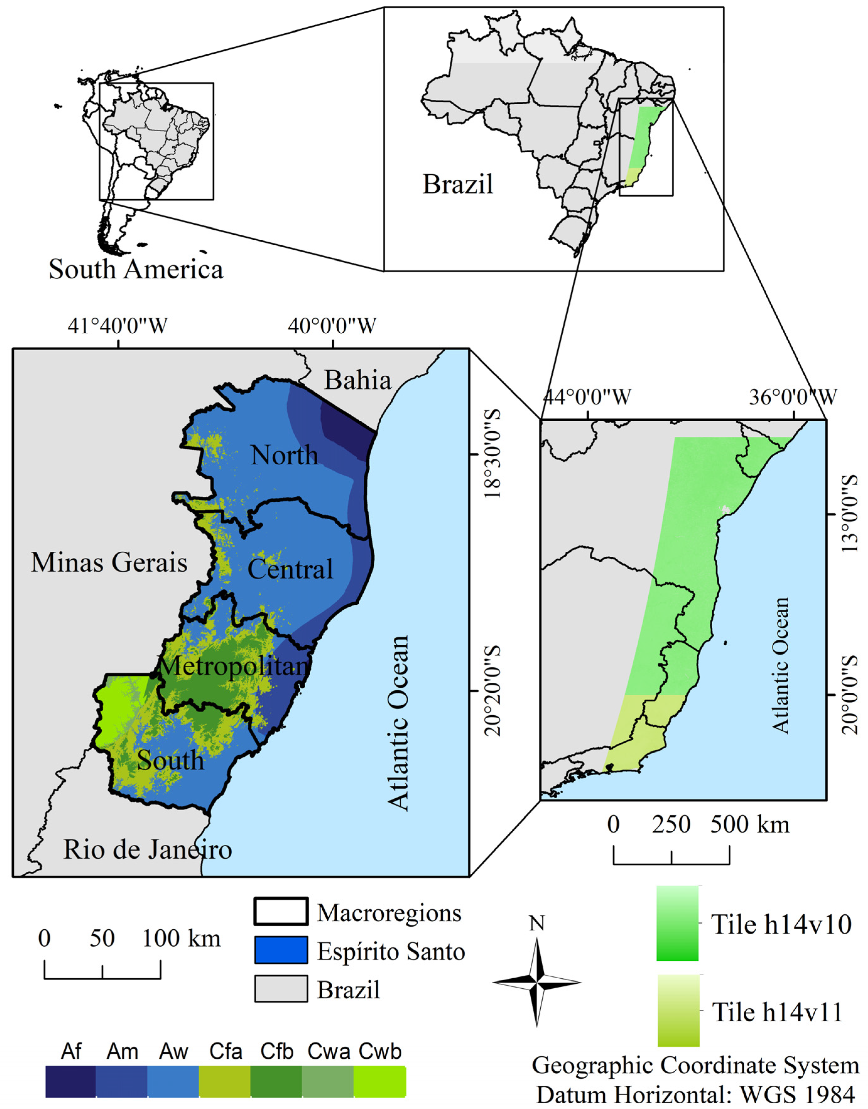
2.1. Study Area

This research was conducted in the State of Espírito Santo, southeastern Brazil, which is surrounded by the states of Bahia, Rio de Janeiro, and Minas Gerais, including the Atlantic Ocean (parallels 17.9° S and 21.3° S and meridians 39.6° W and 41.8° W) (Figure 1).

In view of Köppen’s classification, the Aw climate (tropical zone, with a dry winter) covers the Espírito Santo’s largest area (53.69%). The following climate zones are also found in the study area: Cfa—oceanic climate, without a dry season (14.92%); Am—tropical zone, with a monsoon period (13.96%); Cfb—oceanic climate, without a dry season, though with a temperate summer (10.47%); Cwb—humid temperate climate, with a dry winter and temperate summer (3.36%); Af—humid tropical climate (2.76%); Cwa—humid temperate climate, with a dry winter and hot summer (0.83%); and Cwc—humid temperate climate, with a dry winter and short, cool summer (0.02%) [54].

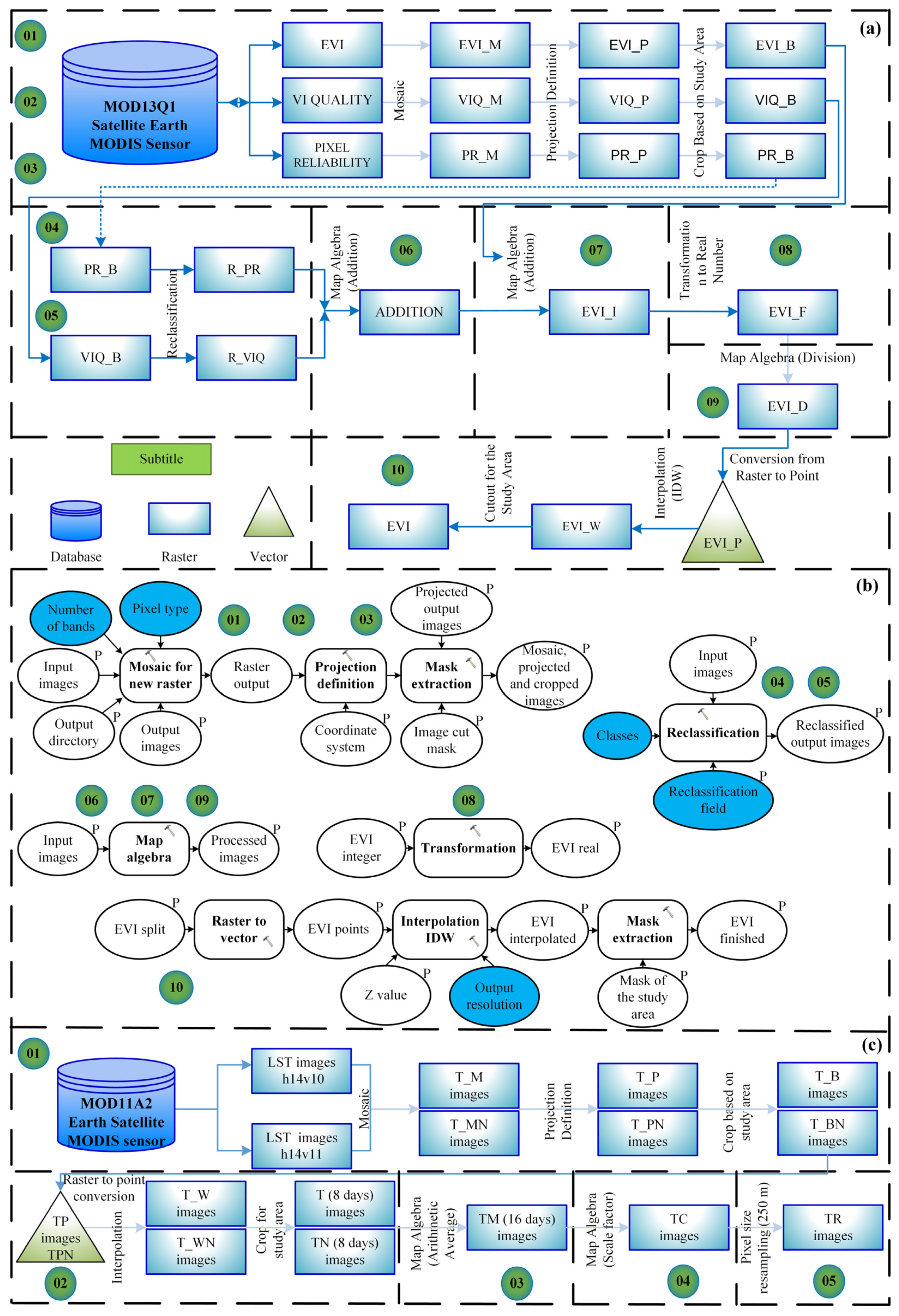
2.2. Acquisition and Processing of Satellite Images from the Selected Vegetation Index

We selected the EVI images, which had a 250 m spatial resolution, and a 16 day temporal resolution, available for free at: https://search.earthdata.nasa.gov, (accessed on 13 October 2022). Version V06 was considered for the data sets, corresponding to the h14v10 and h14v11 tiles. Each tile covers 1200 × 1200 km (Figure 1) [55]. We also opted for images covering the 10 year period of 2008–2017 (

Table 1. Dates of the MODIS images.

Image Years	Start Date (Julian Day)
From 2008 to 2017	01/01 (01), 01/17 (17), 02/02 (33), 02/18 (49), * 03/06 (65), 03/22 (81), 04/07 (97), 04/23 (113), 05/09 (129), 05/25 (145), 06/10 (161), 06/26 (177), 07/12 (193), 07/28 (209), 08/13 (225), 08/29 (241), 09/14 (257), 09/30 (273), 10/16 (289), 11/01 (305), 11/17 (321), 12/03 (337), 12/19 (353)

* From this date on, one day less was considered for each initial date in leap years.

), especially due to the occurrence of the 2014–2016 El Niño event [52,53]. A total of 230 images for each of the layers were processed and used as data sources [56], whereas all geoprocessing procedures and image editing work were performed through ArcGIS 10.3 [57].

A methodological flowchart describing the necessary steps for the processing of EVI images, along with their VI quality and pixel reliability, is presented in Figure 2a, accompanied by a synthesis of the model developed for the automation and documentation of data management processes [58] (Figure 2b), as well as the steps for the processing of the LST images (Figure 2c).

The model was divided into ten steps: (1) we composed a mosaic from each of the layers; (2) the sinusoidal projection was changed to the Universal Transverse Mercator (UTM) system; (3) images were clipped; (4) classification of the pixel reliability (

Table 2. Pixel reliability values for the EVI.

Pixel Value	Quality	Description	Value after Reclassification
−1	No data	Unprocessed data	No data
0	Good data	Can be used with confidence	0
1	Marginal data	* Can be used	0
2	Snow/ice	Target covered by snow or ice	No data
3	Cloud	Cloud covered target	No data

* Observe other quality information. Source: [55], author’s adaptation.

), with the aim of extracting “spurious” pixels by ensuring the data quality and consistency [59]; (5) reclassification of the image quality, and the valid range was from 4 to 37,572 [60]; (6) reclassified images were explored to create a “correction mask”; (7) EVI images were added along with the correction mask, since it is important to eliminate pixels that have been affected by clouds or atmospheric noise in the previous steps [61]; (8) images were converted to float values; (9) images were rescheduled to digital values −1 to +1; (10) images were converted to vector, interpolated by the Inverse Distance Weighted (IDW) method [62], and cut based on the study area [63].

By studying trends in vegetation development, researchers [64] used NDVI data from the National Oceanic and Atmospheric Administration (NOAA) satellite and performed a similar method, eliminating pixels identified as snow or clouds in the images and eventually filling in the gaps with interpolation techniques.

The data geoprocessing model provided the automation and interconnection of different stages, and, by consequence, underwent slight changes to process all 460 EVI images, their VI quality, and pixel reliability. Such an occurrence highlights the possibility of adapting the same model for other research purposes.

2.3. Acquisition and Processing of the Land Surface Temperature Images

Figure 2c shows the steps for the acquisition of LST images, originally with a spatial resolution of 1 km and a temporal resolution of 8 days [55], in addition to the preprocessing carried out similarly to the ones involving EVI images. Therefore, another model was implemented in five steps: (1) For each year, 184 images were utilized to generate a mosaic, resulting in 92 images. In the meantime, the images were redesigned according to the reference World Geodetic System (WGS) 84, zone 24 S, and lastly cut. (2) The images were converted to vector, interpolated through the IDW method [62], and cut based on the study area [63]. (3) The integration was applied to generate the average images for 16 days, resulting in 23 images for each year. (4) The original data in the Kelvin scale were converted into degrees Celsius (°C), according to Equation (1). (5) The images were resampled to a resolution of 250 m.

$$\mathrm{TC}=\mathrm{TM} \times 0.02-273.15$$

(1)

where TC is the pixel value in °C, and TM is the original pixel value in Kelvin.

2.4. Composition, Classification, and Spatialization of the Vegetation Condition Index

For calculating the VCI, with the subsequent definition and spatialization of drought classes, we performed the following steps: (1) The vector files of Espírito Santo, urban spot, and water body [63] were dissolved and updated. (2) The vector images were turned into raster ones. (3) The raster images were reclassified, assigning 0 for the entire Espírito Santo land area, except for urban spot (1) and water body (2), creating a “mask”. (4) The EVI images were added to the “mask”. (5) The images composed of the 16 day temporal resolution were grouped, resulting in 6 images each season (

Table 3. Seasons and initial date of the composition of the EVI images (Julian day).

Summer From December 19 to March 21	Fall From March 22 to June 25	Winter From June 26 to September 29	Spring From September 14 to December 18
12/19 (353)	03/22 (81)	06/26 (177)	09/14 (257)
01/01 (01)	04/07 (97)	07/12 (193)	09/30 (273)
01/17 (17)	04/23 (113)	07/28 (209)	10/16 (289)
02/02 (33)	05/09 (129)	08/13 (225)	11/01 (305)
02/18 (49)	05/25 (145)	08/29 (241)	11/17 (321)
* 03/06 (65)	06/10(161)	09/14 (257)	12/03 (337)

* From this day on, one day less was considered for each initial date in leap years.

). While 23 images were generated annually, the one taken on September 14 was used both in late winter and early spring, as it was the image that covered more days of the two seasons. (6) We calculated the averages of the six images that make up each season of the year for a 10 year period. (7) The averages of the maximum pixel values for 10 summers, falls, winters, and springs were calculated, as we adopted the same procedure for the average of the minimum values. (8) We calculated the VCI for each of the four seasons of the year [15], from 2008 to 2017 (Equation (2)). (9) The VCI was reclassified for each generated index value, according to assumptions of the different drought classes [65] (

Table 4. Class ranges of the VCI values and their corresponding classifications.

VCI Values (%)	Classification
0 < VCI < 20	Extremely dry
20 ≤ VCI < 40	Dry
40 ≤ VCI < 60	Normal condition
60 ≤ VCI < 80	Good condition
VCI ≥ 80	Optimal condition

Source: [65], adapted by the authors.

). (10) Based on the VCI, it was possible to analyze the spatial distribution of the drought occurrence classes, primarily for the most vulnerable conditions in which vegetation is strongly affected by water stress. Since the analysis considered the 2008–2017 timeframe, with a value of the VCI for each season of the year, 40 images were obtained over 10 years.

$$\mathrm{VCI} =\frac{{\overline{\mathrm{x}}}_{\mathrm{v}}-{\overline{\mathrm{x}}}_{\mathrm{ref}\min }}{{\overline{\mathrm{x}}}_{\mathrm{ref}\max }-{\overline{\mathrm{x}}}_{\mathrm{ref}\min }}\times 100$$

(2)

where $\mathrm{VCI}$(%); ${\overline{\mathrm{x}}}_{\mathrm{v}}$ is the average of the EVI pixels arranged by season for a given year; ${\overline{\mathrm{x}}}_{\mathrm{ref}\min }$ is the average of the EVI pixels, with minimum values each season, for a 10 year series; finally, ${\overline{\mathrm{x}}}_{\mathrm{ref}\max }$ is the average of the EVI pixels, with the maximum values of each season, for 10 years.

VCI represents the percentage of the vegetation index that is used, in this case of the EVI, in relation to its maximum amplitude. It is employed for drought monitoring, based on the assumption that the vegetative vigor is affected by weather variations. Thus, in extremely dry periods, vegetation growth is relatively slow, leading to a lower VCI value. On the other hand, a larger VCI represents conditions more suitable to plant growth [30].

The classification and spatialization of droughts, pixel by pixel, aims to provide a view of the spatial and temporal distributions of drought occurrences throughout the study area, together with the characterization of the drought intensity.

2.5. Calculation and Spatialization of Anomalies of the Land Surface Temperature

With the purpose of obtaining the spatial distribution of the LST variations in relation to the average, focusing on the 2008–2017 timeframe, the average values of the LST were calculated for each of the 10 years and the 4 seasons, as well as the reference average of the LST in the season, for the entire 10 year period. From such averages, LST anomalies were calculated using Equation (3), and their spatialization was performed for the study area.

$$\mathrm{Anom} \mathrm{LST}={ \mathrm{LST}}_{\mathrm{v}}-{\mathrm{LST}}_{\mathrm{ref}}$$

(3)

where $\mathrm{Anom} \mathrm{LST}$ represents the land surface temperature anomaly; ${ \mathrm{LST}}_{\mathrm{v}}$ is the average LST of the season analyzed in a given year; and ${\mathrm{LST}}_{\mathrm{ref}}$ is the reference average for each season, that is, the average of that season for a 10 year period.

With the VCI images being subdivided into drought classes, as well as the spatialization images of the LST anomalies, an analysis of the spatiotemporal distribution of these 2 variables was carried out. Such analysis aimed at verifying the areas and seasons of the years with the greatest drought extensions during the study period. These results were also compared with water surplus and deficit data, which were obtained through the water balance performed for the Automatic Meteorological Stations (AMS) closest to the vulnerable regions.

2.6. Statistical Analysis of the Vegetation Condition Index and Land Surface Temperature Data

To obtain the mean values of the VCI and LST, 250 points were generated in each planning macroregion, except in urban areas and water bodies, i.e., 1000 random points were generated throughout the Espírito Santo land area, creating tables with VCI and LST data according to the analysis to be performed.

Through the VCI composition stage, 40 images were obtained and grouped by season, from 2008 to 2017. We adopted the same procedure for the processing of the LST images and, as a result, generating 40 images as well. As long as 1000 random points were generated, there were a total of 40,000 VCI and LST values available for use in the statistical analysis.

The comparison between the mean values of the VCI and LST in the different approaches applied in this research was carried out through analysis of variance, being shortly after followed by normality and homoscedasticity analyses of the residues. At last, the aforementioned methodological approach [66] was applied through the software R [67]. For all analyses, an α equal to 0.05 was established.

In one of the analyses, we compared the value of the VCI averages for each year, from 2008 to 2017. The VCI averages were also compared by season and by each of Espírito Santo’s planning macroregions. Eventually, the average values were compared by macroregion for the worst scenarios obtained in the spatialization of the VCI, i.e., in relation to the most vulnerable periods of drought.

Analyses were also carried out to compare the value of LST averages in each year and also by season and by each of Espírito Santo’s planning macroregions.

In the analysis of variance, the following hypotheses were tested: H₀—the pairs of means are statistically equal; H₁—at least one of the pairs of means are statistically different from each other. If the p-value is lower than the established α, H₀ is rejected, and the analysis continues, applying the Scott–Knott grouping method.

The aforementioned method, in addition to being applied for the univariate analysis and allowing for multiple comparisons efficiently, was brought into light in this research for the following reasons: (1) it is more functionable than the Tukey, Student’s t-, and Duncan tests, as well as several others methods; (2) it has type I error rates that almost always fit in with the nominal levels in various distributions; (3) it enables the interpretation of the results due to the lack of ambiguity; and (4) it is robust in response to the violation of normality [68].

The Scott–Knott method performs a comparison of means through groups that classify them in a homogeneous way [69], based on the likelihood ratio to test the significance that “n” treatments can be divided into two groups that maximize the sum of squares between groups and minimize within them.

In summary, the process consists of determining a partition in two groups, with verification of the partition that maximizes the sum of squares. The number of partitions is given by (2ⁿ⁻¹ − 1). It is easy to obtain all groups for a small number of treatments; however, for a larger one, it means that the number of groups grows exponentially. To circle such an obstacle, it is necessary to order the averages of the treatments and consider only (n − 1) partitions [70]. After finding the best partition between the two groups, the process is repeated in each subgroup until the groups are considered statistically equal by the chi-square test.

This method can be described as follows [66]:

(1) Ordering of the means and determination of the (g − 1) partitions with two groups, considering, initially, that the total number of treatments (n) is equal to the number of treatments involved in the groups of means (g).

(2) Definition of the hypotheses: H₀—G₁ = G₂ and H₁—G₁ ≠ G₂, where G₁ and G₂ are the total number of treatments in each of the two groups of means.

(3) Obtaining the sum of squares (B₀), which is estimated using Equation (4), with verification of the partition that maximizes the sum of squares.

$${\mathrm{B}}_0=\frac{{\mathrm{G}}_1{}^2}{{\mathrm{k}}_1}+\frac{{\mathrm{G}}_2{}^2}{{\mathrm{k}}_2}-\frac{{\left({\mathrm{G}}_1+{\mathrm{G}}_2\right)}^2}{{\mathrm{k}}_1+{\mathrm{k}}_2} , {\mathrm{G}}_1={\sum }_{\mathrm{i}=1}^{{\mathrm{k}}_1}\overline{{\mathrm{Y}}_{\mathrm{i}}} \mathrm{e} {\mathrm{G}}_2={\sum }_{\mathrm{i}={\mathrm{k}}_1+1}^{\mathrm{g}}\overline{{\mathrm{Y}}_{\mathrm{i}}}$$

(4)

where $\overline{{\mathrm{Y}}_{\mathrm{i}}}$ is the mean of treatment i, and k₁ and k₂ represent the number of means of each group.

(4) Calculation of the maximum likelihood estimator (${\hat{\mathsf{\sigma }}}_0{}^2)$ using Equation (5).

$${\hat{\mathsf{\sigma }}}_0{}^2=\frac{1}{\mathrm{g}+\mathrm{v}}.\left[{\displaystyle \sum }_{\mathrm{i}=1}^{\mathrm{g}}{\left(\overline{{\mathrm{Y}}_{\mathrm{i}}}-\overline{\mathrm{Y}}\right)}^2+\mathrm{v}.{\mathrm{s}}_{\overline{\mathrm{Y}}}{}^2\right]$$

(5)

where $\overline{\mathrm{Y}}$ is the general average of all treatments involved, ${\mathrm{s}}_{\overline{\mathrm{Y}}}{}^2=\frac{\mathrm{QME}}{\mathrm{r}}$ is the nonbiased estimator of ${\mathsf{\sigma }}_{\overline{\mathrm{Y}}}{}^2$, and v is the degree of freedom of the estimator.

(5) Determination of the value of the statistic test (Equation (6)) for the partition that maximizes B₀.

$$\mathsf{\lambda }=\frac{\mathsf{ᴨ}}{2\left(\mathsf{ᴨ}-2\right)}.\frac{{\mathrm{B}}_0}{{\hat{\mathsf{\sigma }}}_0{}^2}$$

(6)

where ${\hat{\mathsf{\sigma }}}_0{}^2$ is the maximum likelihood estimator of ${\mathsf{\sigma }}_{\overline{\mathrm{Y}}}{}^2$, and ᴨ is the irrational number of the approximate value of 3.14159.

(6) Whether $\mathsf{\lambda }\ge {\mathsf{\chi }}^2{}_{\left(\mathsf{\alpha }; \mathrm{g}/\left(\mathsf{ᴨ}-2\right)\right)}$, the hypothesis that the two groups are equal is rejected, and the alternate hypothesis is accepted.

(7) The two subgroups that have been formed will be subjected separately to the previous steps, with g = k₁ and g = k₂. The process ends when H₀ is accepted (statistically equal by the ${\chi }^2 \mathrm{test}$) or if each subgroup has only one average.

3. Results and Discussion

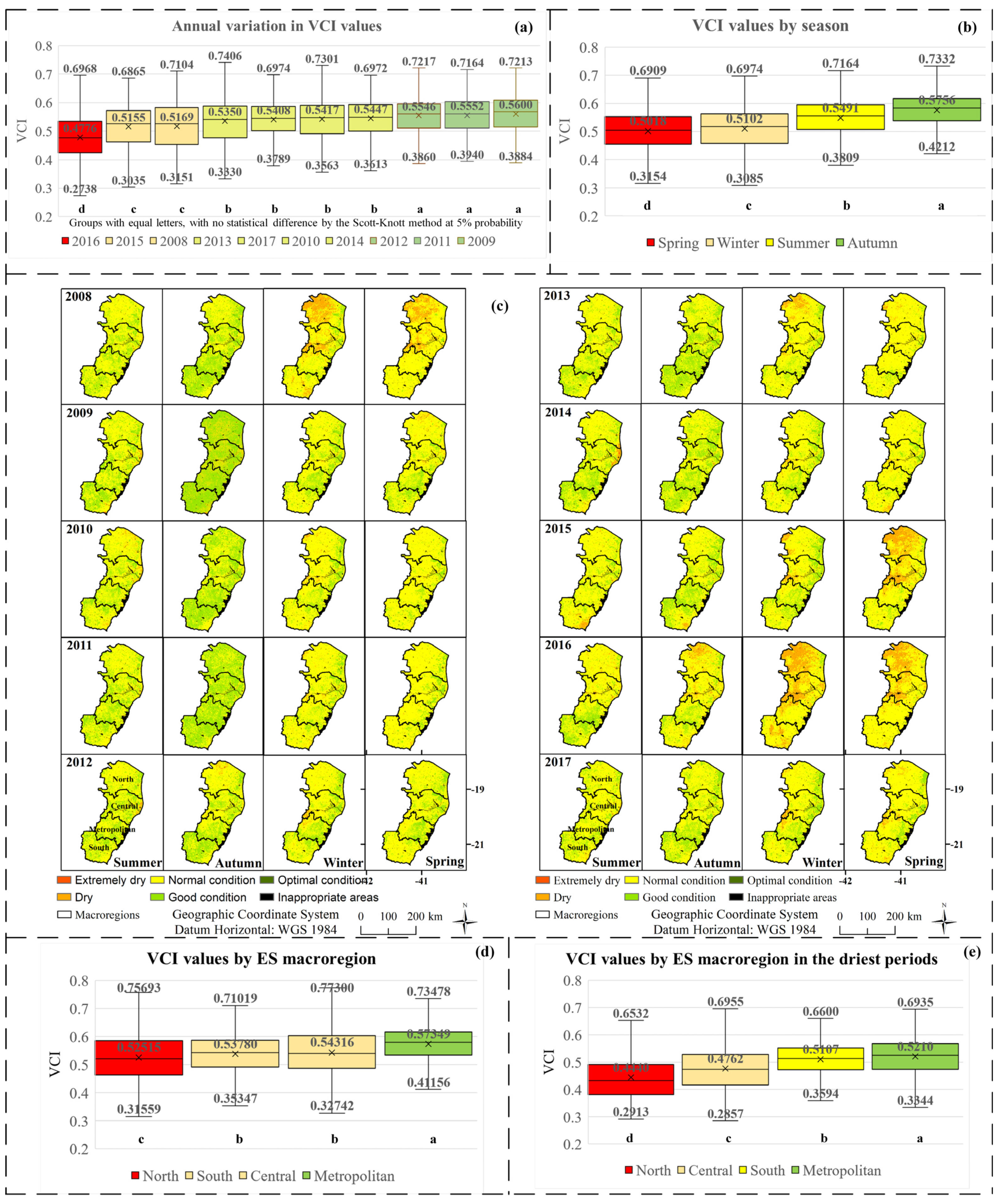
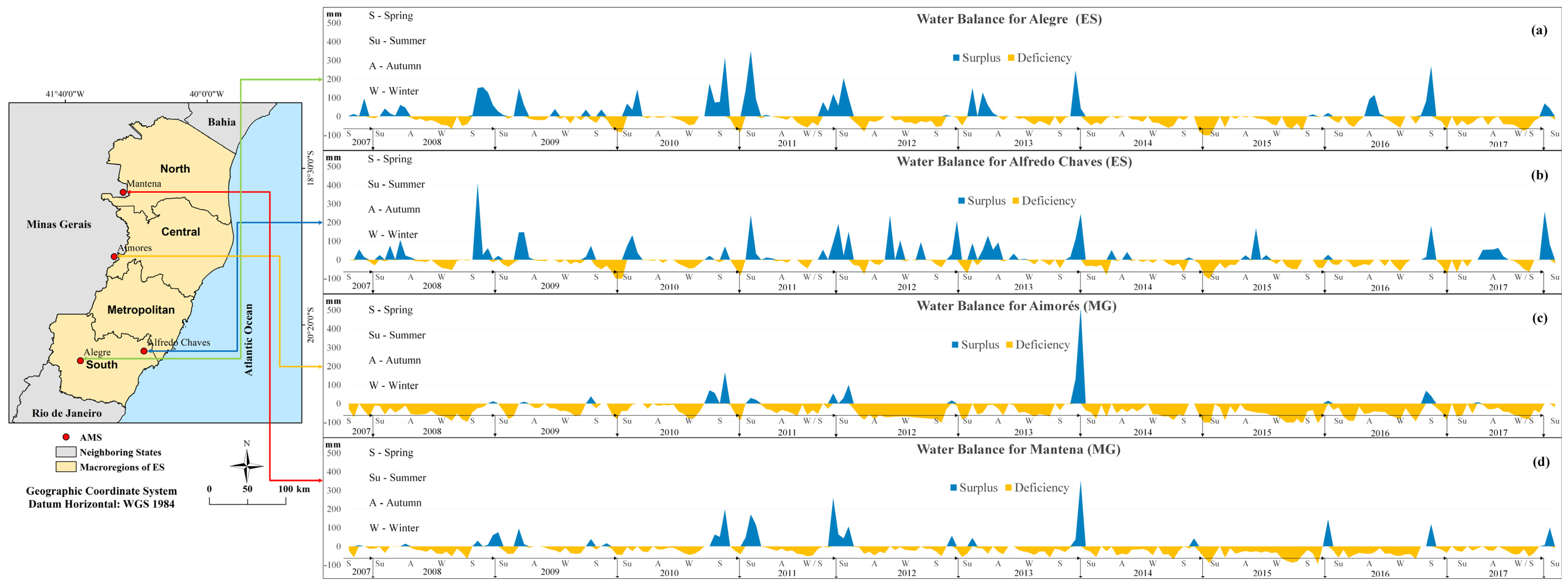
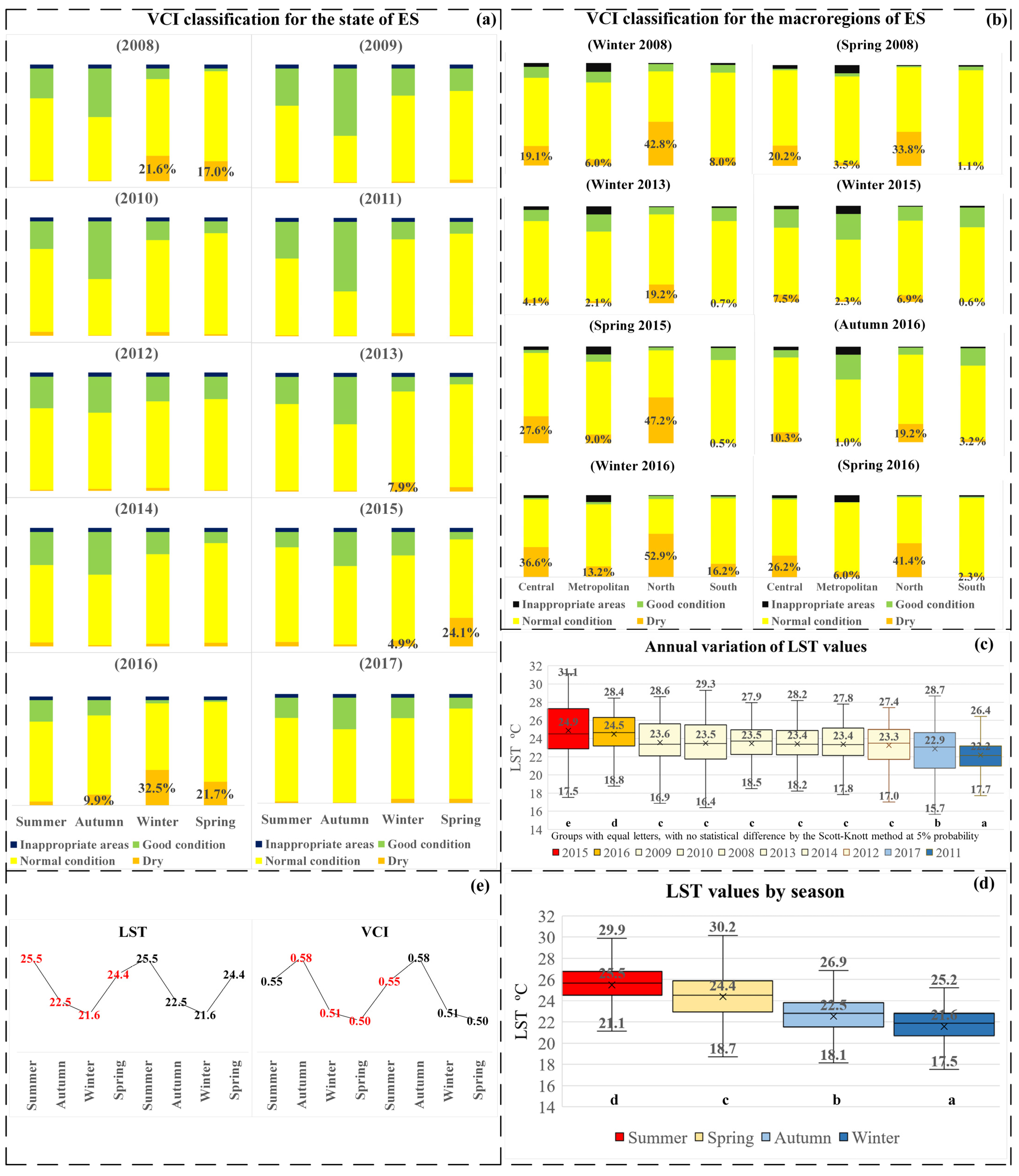
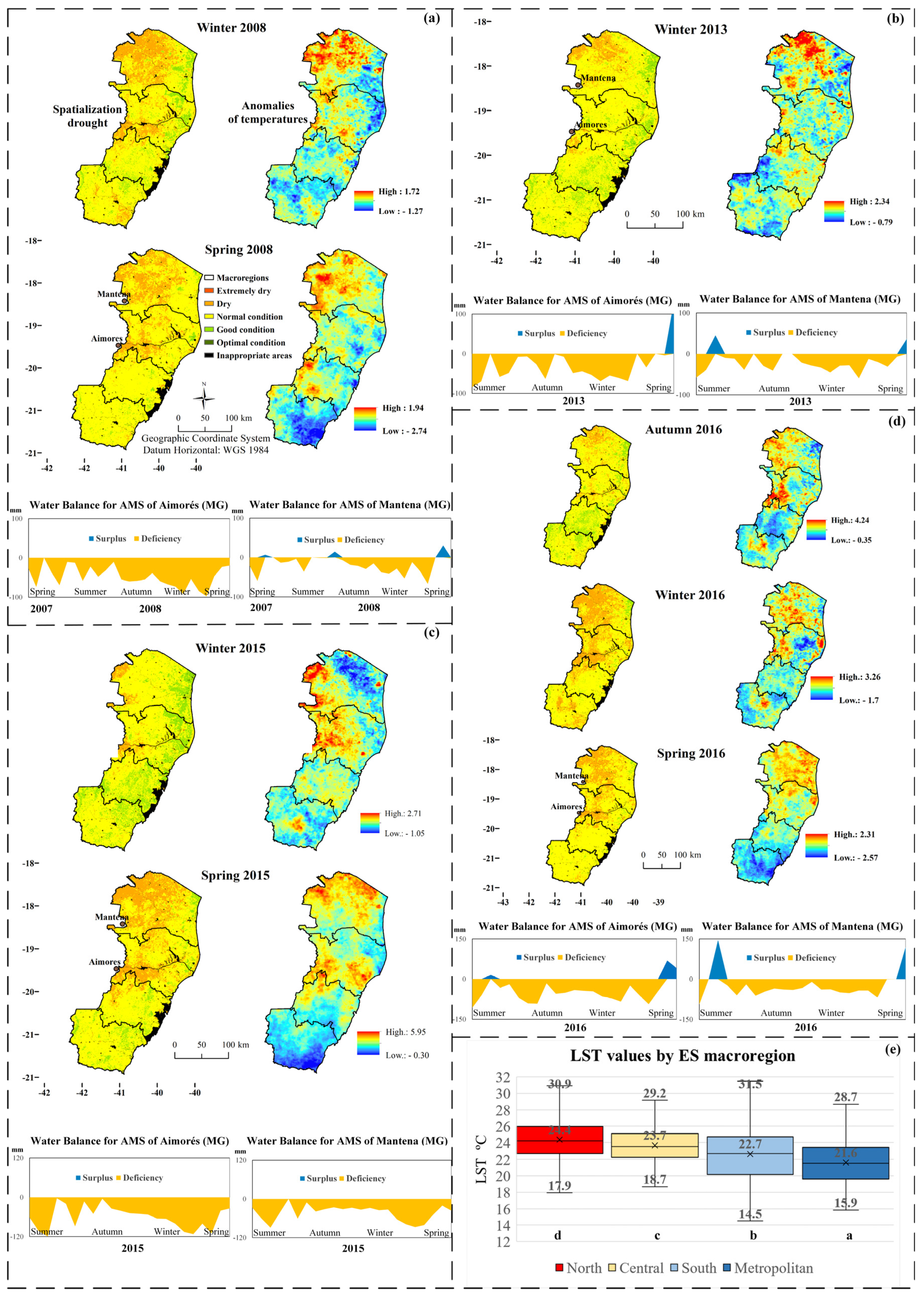
3.1. Analysis and Spatialization of Drought Occurrences for the State of Espírito Santo and Its Macroregions

First, we should emphasize this research study’s limitation, especially when it comes to the short-term timeframe in which we conducted the calculation of the VCI, the values of which are not presented well enough for climatology information. Nevertheless, these values are still meaningful if used as indicators of areas more subject to drought.

Based on the VCI data, we verified the spatialization, identification, and analyses of the occurrences of agricultural drought in Espírito Santo’s macroregion. Figure 3a shows the annual comparison of the VCI values for the study area, from 2008 to 2017, with the separation of the annual averages in the groups that showed statistical differences. Such a method enabled the separation of the mean of the VCI into four groups. Concerning the timeframe, 2016 presented the worst result, as it was considered the driest year in the analyzed period, followed by 2008 and 2015. As for 2010, 2013, 2014, and 2017, they were in an intermediate position, while 2009, 2011, and 2012 obtained the highest mean values of the VCI, indicating better water conditions for vegetation.

The worst VCI results, found in 2015 and 2016, were side by side with the occurrence of strong El Niño events in the same period. Such a phenomenon generally causes an abnormal increase in the temperature in Southeast Brazil, which may have, in turn, caused an increase in water deficiency. By consequence, there were more frequent drought occurrences in Espírito Santo in 2015 and 2016 [52,53].

In addition to the annual comparison of the VCI values, an analysis of the average values by season was performed (Figure 3b). Each of the four seasons showed significant differences in the VCI average, with the lowest results observed in spring and winter and the highest in summer and fall. This shows that even with the beginning of the rainy season in Espírito Santo (typically in spring) [71], the VCI average increased only in the two subsequent seasons (i.e., summer and fall), indicating that there is a delay in the response of the vegetation to the water availability. Similarly, the reduction in precipitation that occurs in fall [72] results in a vegetation response to water deficiency that appears in winter and spring, as indicated by the lower VCI averages. There may be a delay of approximately two months for the vegetation to show an obvious response to water stress [73]; when water stress occurs with high temperatures and high levels of solar radiation, there is a likelihood of significant negative effects on vegetation.

With the aim of verifying the variation of the VCI in a more detailed manner in the study area, Figure 3d shows a comparison of Espírito Santo’s planning macroregion from 2008 to 2017. According to the Scott–Knott method, the separation of the averages into homogeneous groups allows us to observe the existence of three distinct groups: (c) North macroregion, which had the worst mean VCI value and was characterized as the one that suffered the most negative effects of drought occurrence; (b) South and Central macroregions, which had intermediate VCI values without statistically significant differences; finally, (a) Metropolitan macroregion, which had the highest average value, presenting the best water condition.

As a previous study indicated [74], the lower VCI values for the North macroregion were expected based on the fact that water deficiency is one of the primary issues affecting this macroregion, which frequently experiences lower rainfall than the annual average observed across the state. Consequently, there is a deficit in the water balance [72,75,76]. Moreover, certain areas have been subjected to desertification, primarily those located in the Central and Northwest areas from such macroregion [77].

In the Metropolitan macroregion, totally opposite conditions have been verified, with the annual rainfall above the state average, apart from relatively few drought events and a reduced number of areas affected by water deficits [78]. This justifies the higher VCI values.

The only discrepant result in relation to the regional reality concerns the Central macroregion, as it also suffers from drought and has several municipalities frequently affected by desertification [77]. However, considering the dry and rainy seasons, as well as each year in the analysis, they may have increased the VCI mean and caused a result without statistical differences in comparison with the South macroregion.

With the purpose of better visualizing the variations in Espírito Santo’s VCI, as well as in its planning macroregions, Figure 3c presents their spatialization across five drought classes: extremely dry, dry, normal condition, good condition, and optimal condition [65], along with inappropriate areas (i.e., urban and water) for the four seasons of the year, from 2008 to 2012 and from 2013 to 2017.

The VCI represents the percentage of the EVI variation in relation to its maximum amplitude [30]. Thus, the lowest VCI values indicate the driest areas or climatic seasons, where vegetation growth was hampered. By contrast, the highest VCI values indicate the areas or the seasons with the best climatic conditions in which the vegetation presented good development. Thus, using the visual analysis presented in Figure 3c, it can be noted that the data concerning 2008, 2013, 2015, and 2016 presented the greatest areas of drought occurrences, primarily in the Central and North macroregions, as well as during winter and spring. Summer and fall, on the contrary, were the seasons with the best conditions for VCI, as well as the Metropolitan and South macroregions. This suggests that most of the vegetation in these areas showed high vegetative vigor, not suffering water and thermal stress.

As a means to verifying whether the macroregions mentioned in the previous paragraph accurately presented the results indicated in the visual analyses, an additional statistical analysis was carried out with the application of the Scott–Knott method for a supposedly adverse scenario in relation to the VCI spatialization (i.e., for 2008, 2013, 2015, and 2016) in winter and spring (Figure 3e). It should be pointed out that the four macroregions showed averages with significant differences in such a context, corroborating the results of the visual analysis with the lowest VCI value obtained from the North macroregion, followed by the Central, whereas the South and Metropolitan macroregions obtained the best values.

In response to high levels of drought, vegetation undergoes intense stress, resulting in lower VCI values. Thus, in some subsequent analyses, we attempted to place greater emphasis on periods when droughts occurred with greater intensities in the study area.

To confirm whether the VCI spatialization (Figure 3c) presented results according to the local water conditions, the sequential water balance [79] was carried out for a 100 mm of available water capacity [80,81]. By doing so, we employed AMS data from both Alegre and Alfredo Chaves, municipalities located in Espírito Santo’s South macroregion, and also from Aimorés and Mantena, the ones that are close to the Central and North macroregions, despite being located in in the State of Minas Gerais (Figure 4).

In general, it is noteworthy that AMS data from Alegre and Alfredo Chaves had better water conditions than the others, as they are located in Espírito Santo’s Southern macroregion, where the VCI also revealed good results. However, Aimorés’s and Mantena’s AMS indicated a greater water deficit than surplus, in addition to be close to the most vulnerable macroregions according to the VCI values. Therefore, it is possible to note that the VCI exposed the spatial correspondence with local water conditions, configuring itself as an efficient index for the analysis of drought occurrences.

When it comes to the sequential water balance process, 2008, 2013, 2015, and 2016 presented the worst results in the statistical analysis (according to the Scott–Knott clustering method), as a consequence of frequent water deficiencies, mainly in winter and spring, confirming the lower VCI values and the most severe droughts in those periods.

Figure 5a displays the VCI classification for Espírito Santo from 2008 to 2017, with the respective percentages of classes of drought occurrences in the four seasons of the year. Due to the low percentage of occurrence of the extremely dry and optimal condition classes, these were respectively incorporated into the dry and good condition classes.

We ought to emphasize that in 2008, during winter and spring, respectively, 21.6% and 17% of Espírito Santo’s land areas were under drought conditions. In the winter of 2013, a smaller percentage of droughts was observed, which was present in approximately 8.0% of the areas. In 2015, during the spring season, 24.1% of the areas were under drought, while 2016 was marked by one of the worst scenarios in which drought affected approximately 10% of areas in fall, 32.5% in winter, and 21.7% in spring. Once again, these results are consistent with those obtained by the statistical analysis. From 2009 to 2012, 2014, and 2017, across all seasons of the year, more than 90% of the study area had normal and good conditions.

It is worth mentioning that the periods with higher percentages were considered in the analysis of drought occurrence. However, when considering Espírito Santo’s total land area (approximately 46,000 km²), it is clear that by neglecting 1%, this represents an area of approximately 460 km².

Figure 5b shows the VCI classification for the four aforementioned macroregions in the most vulnerable seasons in relation to drought, i.e., winter and spring in 2008; winter in 2013; winter and spring in 2015; and fall, winter, and spring in 2016. Hence, it was possible to identify the macroregions that presented the most and least severe droughts. In almost all of the analyzed periods, the North macroregion displayed the highest percentage of areas affected by drought, followed by the Central one. The Metropolitan and South macroregions had the lowest percentages. These results are in agreement with those groups obtained via the Scott–Knott method.

In 2015 and 2016, the four macroregions presented the highest percentage values of areas affected by drought, primarily during winter and spring; the Central and North macroregions had the highest values, which were approximately 37% and 53%, respectively. The Metropolitan macroregion had a percentage of approximately 13%, while the South macroregion had approximately 16%. As previously mentioned, this was likely a result of the influence of the high-intensity El Niño events that occurred during these timeframes [52,53]. Attention should also be paid to the fact that these events were responsible for the 2015 and 2016 water crises, which caused, during these same years, a drop in production of 9 of the 11 main crops in Espírito Santo [49].

3.2. Interrelationships between Land Surface Temperature and Vegetation Condition Index

The LST is related to the processes of energy balance, evapotranspiration, drought, and desertification. Therefore, it is an important indicator of environmental degradation and climate change; it is also directly related to air temperature and, consequently, to local conditions [82].

Some comparisons were made to analyze the behavior of LST in relation to variations in time and space and the effects on VCI, and Figure 5c shows the annual variation in the LST values for Espírito Santo, from 2008 to 2017, with the separation of the annual averages in groups that showed statistical differences.

As we can see, the LST averages were separated into five groups. The highest average temperature occurred in 2015 and, secondly, in 2016. Intermediate temperatures were measured in 2008, 2009, 2010, 2012, 2013, and 2014, while the lowest LST average could be noted in 2011 and 2017. Based on the significantly higher average temperatures observed in 2015 and 2016, it must be emphasized that the intense El Niño events that occurred during the same period resulted in significantly higher temperatures in southeastern Brazil [52,53].

In addition to the annual comparison of the LST values, an analysis of the average values by season was performed (Figure 5d). The four seasons of the year showed mean LSTs with significant differences (p < 0.05), with the lowest results being observed in fall and winter and the highest in spring and summer.

When comparing the variations in the LST with the variations in the VCI values for the four seasons (Figure 5e), it is notable that the behavior of the VCI variation was identical to that of the LST but with a delay of one season, i.e., the variation of the average VCI values in fall, winter, spring, and summer, in sequence, was the same for the LST in summer, fall, winter, and spring. It should be noted that this may suggest a delay in the response of the vegetation in relation to the LST, but it must be observed concomitantly with the variation in the water conditions (deficit or surplus) for each season, because generally in the seasons when there are increases or decreases in temperature, these changes coincide with increases or decreases in precipitation. When there is an association between a decrease in rainfall and an elevation in temperature, there is a likelihood of a negative influence on the water availability and an increase in the occurrence of drought [83,84].

In order to show the existing relationships between the VCI, water conditions, and LST, the anomalies were calculated for the values of the surface temperature images, which indicate areas with temperatures above and below the average. This comparison was carried out using images of the VCI classes along with the water conditions of the most vulnerable areas. Temperature anomalies play a fundamental role in the occurrence of droughts [85].

Figure 6a–d show the spatialization of the droughts and LST anomalies across Espírito Santo, as well as the respective water balance in two AMS located in or near the most vulnerable areas. We call attention to the values for winter and spring in 2008; winter in 2013; winter and spring in 2015; and fall, winter, and spring in 2016, which were the periods with the highest drought occurrences.

Before analyzing the results, it is important to highlight the fact that the LST values during the day can operate as indicators of the soil moisture content. Essentially, higher LST values may signal lower levels of soil moisture, as water carries a high specific heat. Together with vegetation, water regulates heat exchanges in the soil–atmosphere system. Thus, in dry environments with sparse vegetation, the heat exchange is more pronounced than in humid environments with lush vegetation [86,87].

According to the results, it is possible to observe that, in general, there is a correspondence between the positive anomalies of the LST’s spatial distribution and drought occurrences; essentially, in areas that presented above average soil temperatures, drought occurred at the most severe levels. However, in Figure 6a–d, the area with the lowest temperature anomaly is not the one with optimal conditions, as temperature anomalies are not the only cause of drought. There are other reasons behind this phenomenon, such as precipitation deficiency, erosion, and human activities, including excessive agriculture and deforestation, which can directly trigger aggravating factors, negatively impacting the land’s ability to retain water.

These high temperatures, along with the low rainfall associated with water deficit and other meteorological factors, contribute to important morphological and physiological changes in vegetation, such as premature leaf fall, reduction in leaf area, height, diameter, and vegetative vigor, which are indicators of drought occurrence at the most severe levels [88,89]. These changes in vegetation also influence the VCI, reducing its value and indicating the most vulnerable areas.

Considering the whole analyzed timeframes, the Central and North macroregions showed the most frequent occurrences of drought, as well as the highest positive anomalies of LST. The water balance analysis carried out in the two AMS, located close to the most vulnerable areas, confirms that the local vegetation was intensely affected by water stress, reflected in the reduction in the VCI values. On the other hand, the Metropolitan and South macroregions had the lowest values of LST anomalies and had only a few occurrences of drought.

Several studies have assessed the occurrence of drought through precipitation anomalies [90]. However, as can be noted in the results, LST anomalies have a strong association with drought events and should not be disregarded when performing analyses.

For a more comprehensive analysis, data obtained using orbital precipitation images could have been used, as well as a study [91] that evaluated drought conditions in two regions of the United States using a combination of the MODIS sensor surface temperature and vegetation indices with the precipitation data program Tropical Rainfall Measuring Mission (TRMM). In conclusion, such data may be used to monitor drought in humid and arid regions.

In the final analysis, a comparison of the LST averages was performed for the four macroregions of Espírito Santo (Figure 6e). The Central and North macroregions had the highest LST averages, while the Metropolitan and South had the lowest. Similarly, when comparing the VCI averages by macroregion, the Central and North had the worst values, while the South and Metropolitan had the best. These results show the strong relationship between positive LST anomalies and the spatial distribution of the VCI, while they can be used as indicators of areas most susceptible to drought.

Studies on drought are challenging, including estimates of the qualitative and quantitative measurements of occurrences and the spatiotemporal distribution, especially in extensive land areas, such as in the State of Espírito Santo, which have very different environmental conditions.

4. Conclusions

This research aimed at identifying susceptible areas to agricultural drought in the State of Espírito Santo, Brazil, in order to enhance the understanding of agricultural drought and its effect on vegetation by enabling mitigation actions and management of water resources.

The results of this study indicate that (1) the methodological approach is an efficient alternative for the identification, classification, and spatiotemporal distribution of agricultural drought occurrences, as it allows for the identification of the most vulnerable regions and periods in relation to drought and also to conduct planning and risk management procedures; (2) the Central and North macroregions of Espírito Santo were the most heavily affected by drought events, especially in winter and spring, deserving greater attention from public authorities; (3) positive LST anomalies can be used as indicators of the most vulnerable areas to drought events, but as far as LST anomalies are concerned, they should be analyzed in conjunction with other factors, such as the water availability and land use and occupation; (4) although it has not been related to the aim of this study, we ought to highlight that the Scott–Knott method allows for objectivity in the interpretation of the results of a comparison between the means due to the absence of ambiguity; (5) the periods with the worst results in the statistical analysis were indeed the ones with frequent water deficiencies (validated by sequential water balance), confirming the lower VCI values and the most severe droughts in these phases; finally, (6) the proposed methodology can be applied to other Brazilian regions and to drought-affected areas in other countries.

References

1. Dai, A. Erratum: Drought under Global Warming: A Review. Wiley Interdiscip. Rev. Clim. Chang. 2012, 3, 617. [Google Scholar] [CrossRef] [Green Version]
2. Riebsame, W.E.; Changnon, S.A.; Karl, T.R. Drought and Natural Resources Management in the United States: Impacts and Implications of the 1987-89 Drought; Westview Press: Boulder, CO, USA, 2019; ISBN 9780429694547. [Google Scholar]
3. Santos, R.B.d.; Menezes, J.A.; Confalonieri, U.; Madureira, A.P.; Duval, I.d.B.; Garcia, P.P.; Margonari, C. Construção e Aplicação de um Índice de Vulnerabilidade Humana à Mudança do Clima para o Contexto Brasileiro: A Experiência do Estado do Espírito Santo. Saúde e Soc. 2019, 28, 299–321. [Google Scholar] [CrossRef]
4. Xu, H.; Wang, X.; Zhao, C.; Yang, X. Assessing the Response of Vegetation Photosynthesis to Meteorological Drought across Northern China. L. Degrad. Dev. 2021, 32, 20–34. [Google Scholar] [CrossRef]
5. Lesk, C.; Rowhani, P.; Ramankutty, N. Influence of Extreme Weather Disasters on Global Crop Production. Nature 2016, 529, 84–87. [Google Scholar] [CrossRef] [Green Version]
6. FAO. Disasters Causing Billions in Agricultural Losses, with Drought Leading the Way. FAO in Geneva. Organización de Las Naciones Unidas Para La Alimentación y La Agricultura. 2018. Available online: https://www.fao.org/geneva/news/detail/es/c/1109572/ (accessed on 30 December 2022).
7. Faria, S.M. O Fenômeno Seca e a Produtividade Agrícola do Estado de Goiás; Universidade Federal de Goiás: Goiás, Brazil, 2011. [Google Scholar]
8. Lawal, S.; Hewitson, B.; Egbebiyi, T.S.; Adesuyi, A. On the Suitability of Using Vegetation Indices to Monitor the Response of Africa’s Terrestrial Ecoregions to Drought. Sci. Total Environ. 2021, 792, 148282. [Google Scholar] [CrossRef]
9. Vivas, E.B.d.F. Avaliação e Gestão de Situações de Seca e Escassez: Aplicação ao Caso do Guadiana; Universidade do Porto: Porto, Portugal, 2011. [Google Scholar]
10. Van Quang, N.; Long, D.T.; Anh, N.D.; Hai, T.N. Administrative Capacity of Local Government in Responding to Natural Disasters in Developing Countries. J. Hum. Earth Futur. 2021, 2, 114–124. [Google Scholar] [CrossRef]
11. Pereira, A.R.; Angelocci, L.R.; Sentelhas, P.C. Agrometeorologia: Fundamentos e Aplicações Práticas; Agropecuária: Guaíba, Brazil, 2002. [Google Scholar]
12. Sandeep, P.; Obi Reddy, G.P.; Jegankumar, R.; Arun Kumar, K.C. Monitoring of Agricultural Drought in Semi-Arid Ecosystem of Peninsular India through Indices Derived from Time-Series CHIRPS and MODIS Datasets. Ecol. Indic. 2021, 121, 107033. [Google Scholar] [CrossRef]
13. Sousa Júnior, M.A.; Sausen, T.M.; Lacruz, M.S.P. Monitoramento de Estiagem na Região Sul do Brasil Utilizando Dados ENVI/MODIS no Período de Dezembro de 2000 a Junho de 2009; Instituto Nacional de Pesquisas Espaciais–INPE: São José dos Campos, Brazil, 2011. [Google Scholar]
14. Huete, A.; Didan, K.; Miura, T.; Rodriguez, E.P.; Gao, X.; Ferreira, L.G. Overview of the Radiometric and Biophysical Performance of the MODIS Vegetation Indices. Remote Sens. Environ. 2002, 83, 195–213. [Google Scholar] [CrossRef]
15. Kogan, F.N. Application of Vegetation Index and Brightness Temperature for Drought Detection. Adv. Sp. Res. 1995, 15, 91–100. [Google Scholar] [CrossRef]
16. Wang, W.; Wang, W.J.; Li, J.S.; Wu, H.; Xu, C.; Liu, T. The Impact of Sustained Drought on Vegetation Ecosystem in Southwest China Based on Remote Sensing. Procedia Environ. Sci. 2010, 2, 1679–1691. [Google Scholar] [CrossRef] [Green Version]
17. Ginciene, B.R.; Bitencourt, M.D. Utilização do EVI (Enhanced Vegetation Index) para Maior Sensibilidade na Detecção de Mudanças Temporais em Fragmentos de Floresta Estacional Semidecidual. In Proceedings of the Simpósio Brasileiro de Sensoriamento Remoto, Curitiba, Brazil, 28–31 November 2011. [Google Scholar]
18. Marcuzzo, F.F.N.; Goularte, E.R.P. Índice de Anomalia de Chuvas do Estado do Tocantins. Geoambiente Jataí–GO 2012, 19, 55–71. [Google Scholar]
19. Wu, J.; Zhou, L.; Liu, M.; Zhang, J.; Leng, S.; Diao, C. Establishing and Assessing the Integrated Surface Drought Index (ISDI) for Agricultural Drought Monitoring in Mideastern China. Int. J. Appl. Earth Obs. Geoinf. 2013, 23, 397–410. [Google Scholar] [CrossRef]
20. Yoshida, Y.; Joiner, J.; Tucker, C.; Berry, J.; Lee, J.E.; Walker, G.; Reichle, R.; Koster, R.; Lyapustin, A.; Wang, Y. The 2010 Russian Drought Impact on Satellite Measurements of Solar-Induced Chlorophyll Fluorescence: Insights from Modeling and Comparisons with Parameters Derived from Satellite Reflectances. Remote Sens. Environ. 2015, 166, 163–177. [Google Scholar] [CrossRef]
21. Wang, S.; Huang, C.; Zhang, L.; Lin, Y.; Cen, Y.; Wu, T. Monitoring and Assessing the 2012 Drought in the Great Plains: Analyzing Satellite-Retrieved Solar-Induced Chlorophyll Fluorescence, Drought Indices, and Gross Primary Production. Remote Sens. 2016, 8, 61. [Google Scholar] [CrossRef] [Green Version]
22. Han, Z.; Huang, Q.; Huang, S.; Leng, G.; Bai, Q.; Liang, H.; Wang, L.; Zhao, J.; Fang, W. Spatial-Temporal Dynamics of Agricultural Drought in the Loess Plateau under a Changing Environment: Characteristics and Potential Influencing Factors. Agric. Water Manag. 2021, 244, 106540. [Google Scholar] [CrossRef]
23. Liu, L.; Yang, X.; Zhou, H.; Liu, S.; Zhou, L.; Li, X.; Yang, J.; Han, X.; Wu, J. Evaluating the Utility of Solar-Induced Chlorophyll Fluorescence for Drought Monitoring by Comparison with NDVI Derived from Wheat Canopy. Sci. Total Environ. 2018, 625, 1208–1217. [Google Scholar] [CrossRef]
24. Liu, Q.; Zhang, S.; Zhang, H.; Bai, Y.; Zhang, J. Monitoring Drought Using Composite Drought Indices Based on Remote Sensing. Sci. Total Environ. 2020, 711, 134585. [Google Scholar] [CrossRef]
25. Zhou, X.; Wang, P.; Tansey, K.; Zhang, S.; Li, H.; Wang, L. Developing a Fused Vegetation Temperature Condition Index for Drought Monitoring at Field Scales Using Sentinel-2 and MODIS Imagery. Comput. Electron. Agric. 2020, 168, 105144. [Google Scholar] [CrossRef]
26. Gao, X.; Huete, A.R.; Ni, W.; Miura, T. Optical-Biophysical Relationships of Vegetation Spectra without Background Contamination. Remote Sens. Environ. 2000, 74, 609–620. [Google Scholar] [CrossRef]
27. Justice, C.O.; Townshend, J.R.G.; Vermote, E.F.; Masuoka, E.; Wolfe, R.E.; Saleous, N.; Roy, D.P.; Morisette, J.T. An Overview of MODIS Land Data Processing and Product Status. Remote Sens. Environ. 2002, 83, 3–15. [Google Scholar] [CrossRef]
28. Aulia, M.R.; Liyantono; Setiawan, Y.; Fatikhunnada, A. Drought Detection of West Java’s Paddy Field Using MODIS EVI Satellite Images (Case Study: Rancaekek and Rancaekek Wetan). Procedia Environ. Sci. 2016, 33, 646–653. [Google Scholar] [CrossRef] [Green Version]
29. Gonçalves, N.B.; Lopes, A.P.; Dalagnol, R.; Wu, J.; Pinho, D.M.; Nelson, B.W. Both Near-Surface and Satellite Remote Sensing Confirm Drought Legacy Effect on Tropical Forest Leaf Phenology after 2015/2016 ENSO Drought. Remote Sens. Environ. 2020, 237, 111489. [Google Scholar] [CrossRef]
30. Du, L.; Tian, Q.; Yu, T.; Meng, Q.; Jancso, T.; Udvardy, P.; Huang, Y. A Comprehensive Drought Monitoring Method Integrating MODIS and TRMM Data. Int. J. Appl. Earth Obs. Geoinf. 2013, 23, 245–253. [Google Scholar] [CrossRef]
31. Zhuo, Z.Y.; Long, Q.B.; Bai, P. Scale of Meteorological Drought Index Suitable for Characterizing Agricultural Drought: A Case Study of Hunan Province. J. South-to-North Water Transf. Water Sci. Technol. 2021, 19, 119–128. [Google Scholar]
32. Patel, N.R.; Yadav, K. Monitoring Spatio-Temporal Pattern of Drought Stress Using Integrated Drought Index over Bundelkhand Region, India. Nat. Hazards 2015, 77, 663–677. [Google Scholar] [CrossRef]
33. Shamsipour, A.A.; Zawar-Reza, P.; Alavi Panah, S.K.; Azizi, G. Analysis of Drought Events for the Semi-Arid Central Plains of Iran with Satellite and Meteorological Based Indicators. Int. J. Remote Sens. 2011, 32, 9559–9569. [Google Scholar] [CrossRef]
34. Sha, S.; Guo, N.; Li, Y.H.; Ren, Y.L.; Li, Y.P. Comparison of the Vegetation Condition Index with Meteorological Drought Indices: A Case Study in Henan Province. J. Glaciol. Geocryol. 2013, 35, 990–998. [Google Scholar]
35. Li, X.-Y.; Yang, L.-A.; Nie, H.-M.; Ren, L.; Hu, S.; Yang, Y.-C. Assessment of Temporal and Spatial Dynamics of Agricultural Drought in Shaanxi Province Based on Vegetation Condition Index. Chin. J. Ecol. 2018, 37, 1172–1180. [Google Scholar] [CrossRef]
36. Quiring, S.M.; Ganesh, S. Evaluating the Utility of the Vegetation Condition Index (VCI) for Monitoring Meteorological Drought in Texas. Agric. For. Meteorol. 2010, 150, 330–339. [Google Scholar] [CrossRef]
37. Agutu, N.O.; Awange, J.L.; Ndehedehe, C.; Mwaniki, M. Consistency of Agricultural Drought Characterization over Upper Greater Horn of Africa (1982–2013): Topographical, Gauge Density, and Model Forcing Influence. Sci. Total Environ. 2020, 709, 135149. [Google Scholar] [CrossRef]
38. Walz, Y.; Min, A.; Dall, K.; Duguru, M.; Villagran de Leon, J.-C.; Graw, V.; Dubovyk, O.; Sebesvari, Z.; Jordaan, A.; Post, J. Monitoring Progress of the Sendai Framework Using a Geospatial Model: The Example of People Affected by Agricultural Droughts in Eastern Cape, South Africa. Prog. Disaster Sci. 2020, 5, 100062. [Google Scholar] [CrossRef]
39. Hu, T.; Renzullo, L.J.; van Dijk, A.I.J.M.; He, J.; Tian, S.; Xu, Z.; Zhou, J.; Liu, T.; Liu, Q. Monitoring Agricultural Drought in Australia Using MTSAT-2 Land Surface Temperature Retrievals. Remote Sens. Environ. 2020, 236, 111419. [Google Scholar] [CrossRef]
40. Ji, M.; Zhang, C.; Zhao, J.W.; Yan, J.L.L. Temporal and Spatial Dynamics of Spring Drought in Qinghai-Tibet Region Based on VCI Index. Remote Sens. L. Resour. 2021, 33, 152–157. [Google Scholar] [CrossRef]
41. Quiring, S.M.; Papakryiakou, T.N. An Evaluation of Agricultural Drought Indices for the Canadian Prairies. Agric. For. Meteorol. 2003, 118, 49–62. [Google Scholar] [CrossRef]
42. Lv, X.; Yin, X.; Gong, A.; Wang, Q.; Li, J.; Zhang, H. Temporal and Spatial Analysis of Agricultural Drought in Yunnan Provincebased on Vegetation Condition Index. J. Geo-Inf. Sci. 2016, 18, 1634–1644. [Google Scholar]
43. Sun, X.; Wang, M.; Li, G.; Wang, J.; Fan, Z. Divergent Sensitivities of Spaceborne Solar-Induced Chlorophyll Fluorescence to Drought among Different Seasons and Regions. ISPRS Int. J. Geo-Inf. 2020, 9, 542. [Google Scholar] [CrossRef]
44. Shen, Z.; Zhang, Q.; Singh, V.P.; Sun, P.; Song, C.; Yu, H. Agricultural Drought Monitoring across Inner Mongolia, China: Model Development, Spatiotemporal Patterns and Impacts. J. Hydrol. 2019, 571, 793–804. [Google Scholar] [CrossRef]
45. Marengo, J.A. Caracterização do Clima no Século XX e Cenários Climáticos no Brasil e na América do Sul para o Século XXI Derivados dos Modelos Globais de Clima do IPCC; Revista Multiciência: Campinas, Brazil, 2007. [Google Scholar]
46. ANA. Conjuntura dos Recursos Hídricos no Brasil 2017: Relatório Pleno; Agência Nacional de Águas: Brasília, Brazil, 2017. [Google Scholar]
47. Souza, F.A.O.d; Oliveira, M.M. Panorama dos Danos Humanos Provocados por Secas e Cheias no Brasil e uma Proposta de Regionalização de Investimentos na Gestão de Riscos. Desenvolv. e Meio Ambient. 2019, 51, 282–310. [Google Scholar] [CrossRef] [Green Version]
48. Ceped UFSC. Atlas Brasileiro de Desastres Naturais: 1991 a 2012, 2nd ed.; Volume Espírito Santo; Ceped UFSC: Florianópolis, Brazil, 2013. [Google Scholar]
49. Governo do Estado do Espírito Santo. Panorama Econômico do Espírito Santo: 3o Trimestre de. 2017. Available online: http://www.ijsn.es.gov.br/artigos/4970-panorama-economico-do-espirito-santo-3-trimestre-de-2017 (accessed on 4 February 2020).
50. Silva, A.C.; Pimenta, A.A.G.; Silva Neto, F.B. Histórico de Desastres do Estado do Espírito Santo 2000–2009. Available online: https://defesacivil.es.gov.br/Media/defesacivil/Publicacoes/Livro-Histórico de Desastres do Estado do Espírito Santo-2000 a 2009.pdf (accessed on 4 February 2020).
51. INCAPER. Instituto Capixaba de Pesquisa, Assistência Técnica e Extensão; INCAPER: Vitória, Brazil, 2016.
52. INPE-Instituto Nacional de Pesquisas Espaciais. El Niño e La Niña-CPTEC/INPE. Available online: http://enos.cptec.inpe.br/elnino/pt (accessed on 12 December 2019).
53. NOAA El Nino Related Global Temperature e Precipitation Patterns. Available online: https://origin.cpc.ncep.noaa.gov/products/analysis_monitoring/ensocycle/elninosfc.shtml (accessed on 18 December 2019).
54. Alvares, C.A.; Stape, J.L.; Sentelhas, P.C.; De Moraes Gonçalves, J.L.; Sparovek, G. Köppen’s Climate Classification Map for Brazil. Meteorol Zeitschrift 2013, 22, 711–728. [Google Scholar] [CrossRef]
55. Didan, K.; Munoz, A.B.; Solano, R.; Huete, A. MODIS Vegetation Index User ’s Guide; The University of Arizona Press: Tucson, AZ, USA, 2015. [Google Scholar]
56. dos Santos, A.R.; Eugenio, F.C.; Ribeiro, C.A.A.S.; Soares, V.P.; Moreira, M.A.; dos Santos, G.M.A.D.A. ArcGIS 10.2.2 Passo a Passo: Elaborando Meu Primeiro Mapeamento–Volume 1; CAUFES: Alegre, Brazil, 2014. [Google Scholar]
57. ESRI. ArcGIS Desktop: Release 10.1; Environmental Systems Research Institute: Redlands, CA, USA, 2015. [Google Scholar]
58. AbdelRahman, M.A.E.; Tahoun, S. GIS Model-Builder Based on Comprehensive Geostatistical Approach to Assess Soil Quality. Remote Sens. Appl. Soc. Environ. 2019, 13, 204–214. [Google Scholar] [CrossRef]
59. Moraes, R.A. Monitoramento e Estimativa da Produção da Cultura de Cana-de-Açúcar no Estado de São Paulo por Meio de Dados Espectrais e Agrometeorológicos; Universidade Estadual de Campinas: Campinas, Brazil, 2012. [Google Scholar]
60. Moraes, R.A.; Rocha, J.V. Imagens de Coeficiente de Qualidade (Quality) e de Confiabilidade (Reliability) para Seleção de Pixels em Imagens de NDVI do Sensor MODIS para Monitoramento da Cana-de-Açúcar no Estado de São Paulo. In Proceedings of the XV Simpósio Brasileiro de Sensoriamento Remoto-SBSR, Curitiba, Brazil, 30 April–5 May 2011; pp. 547–552. [Google Scholar]
61. Yu, F.; Price, K.P.; Ellis, J.; Shi, P. Response of Seasonal Vegetation Development to Climatic Variations in Eastern Central Asia. Remote Sens. Environ. 2003, 87, 42–54. [Google Scholar] [CrossRef]
62. Watson, D.F.; Philip, G.M. A Refinement of Inverse Distance Weighted Interpolation. Geoprocessing 1985, 2, 315–327. [Google Scholar]
63. Geobases Sistema Integrado de Bases Geoespaciais do Estado do Espírito Santo. Available online: https://geobases.es.gov.br/downloads (accessed on 12 March 2019).
64. Chen, B.; Xu, G.; Coops, N.C.; Ciais, P.; Innes, J.L.; Wang, G.; Myneni, R.B.; Wang, T.; Krzyzanowski, J.; Li, Q.; et al. Changes in Vegetation Photosynthetic Activity Trends across the Asia-Pacific Region over the Last Three Decades. Remote Sens. Environ. 2014, 144, 28–41. [Google Scholar] [CrossRef]
65. Coleve, P.A. Aplicação de Índices das Condições de Vegetação no Monitoramento em Tempo Quase Real da Seca em Moçambique Usando NOAA_AVHRR-NDVI. GEOUSP–Espaço e Tempo. São Paulo, Brazil 2011, 29, 85–95. [Google Scholar]
66. Scott, A.J.; Knott, M. A Cluster Analysis Method for Grouping Means in the Analysis of Variance. Biometrics 1974, 30, 507. [Google Scholar] [CrossRef] [Green Version]
67. R Development Core Team. R: A Language and Environment for Statistical Computing. Available online: http://www.r-project.org (accessed on 12 March 2019).
68. Borges, L.; Ferreira, D. Power and Type I Errors Rate of Scott–Knott, Tukey and Newman–Keuls Tests under Normal and No-Normal Distributions of the Residues. Rev. Matemática e Estatística 2003, 21, 67–83. [Google Scholar]
69. Ramalho, M.A.P.; Ferreira, D.F.; Oliveira, A.C. Experimentação em Genética e Melhoramento de Plantas; UFLA: Lavras, Brazil, 2000. [Google Scholar]
70. Fisher, W.D. On Grouping for Maximum Homogeneity. J. Am. Stat. Assoc. 1958, 53, 789–798. [Google Scholar] [CrossRef]
71. Brandão, F.D.; Gonçalves, M.; Jabor, P.M. Diagnóstico e o Prognóstico das Condições de Uso da Água na Bacia Hidrográfica do Rio Itapemirim como Subsídio Fundamental ao Enquadramento e Plano de Recursos Hídricos; AGERH: Vitória, Brazil, 2018.
72. ECOPLAN-LUME. Plano Integrado de Recursos Hídricos da Bacia Hidrográfica do Rio Doce e Planos de Ações para as Unidades de Planejamento e Gestão de Recursos Hídricos no Âmbito da Bacia do Rio Doce–Volume I; Consórcio Ecoplan-Lume. Contrato: Porto Alegre, Brazil, 2010. [Google Scholar]
73. Arato, H.D.; Martins, S.V.; Ferrari, S.H.d.S. Produção e Decomposição de Serapilheira em um Sistema Agroflorestal Implantado para Recuperação de Área Degradada em Viçosa-MG. Rev. Árvore 2003, 27, 715–721. [Google Scholar] [CrossRef]
74. IJSN-Governo do Estado do Espírito Santo. Atlas Histórico-Geográfico do Espírito Santo; SEDU/IJSN: Vitória, Brazil, 2011. [Google Scholar]
75. Brandão, F.D.; Gonçalves, M.A.; Jabor, P.M. Diagnóstico e o Prognóstico das Condições de Uso da Água na Bacia Hidrográfica do Rio São Mateus como Subsídio Fundamental ao Enquadramento e Plano de Recursos Hídricos; AGERH: Vitória, Brazil, 2018.
76. Brandão, F.D.; Gonçalves, M.A.; Jabor, P.M. Diagnóstico e o Prognóstico das Condições de Uso da Água na Bacia Hidrográfica do Rio Itaúnas como Subsídio Fundamental ao Enquadramento e Plano de Recursos Hídricos; AGERH: Vitória, Brazil, 2018.
77. Brasil. Coordenadoria Técnica de Combate à Desertificação Programa de Ação Nacional de Combate à Desertificação e Mitigação dos Efeitos da Seca–PAN Brasil; Ministério do Meio Ambiente: Brasília, Brazil, 2005. [Google Scholar]
78. IEMA. Elaboração de Projeto Executivo para Enquadramento dos Corpos de Água em Classes e Plano de Bacia para os Rios Santa Maria da Vitória e Jucu. Relatorio II, Volume II; Secretaria do Meio Ambiente: Vitória, Brazil, 2015. [Google Scholar]
79. Thornthwaite, C.W.; Mather, J. The Water Balance; Drexel Institute of Technology, Laboratory of Climatology: Centerton, NJ, USA, 1955. [Google Scholar]
80. MH COSTA. Balanço Hídrico Segundo Thornthwaite e Mather, 1955; Universidade Federal de Viçosa, Departamento de Engenharia Agrícola. Engenharia na Agricultura, C. Didático 19: Viçosa, Brazil, 1994. [Google Scholar]
81. Rolim, G.; Sentelhas, P.; Barbiere, V. Planilhas no Ambiente EXCEL para os Cálculos de Balanços Hídricos: Normal, Sequencial, de Cultura e de Produtividade Real e Potencial. Rev. Bras. Agrometeorol. 1998, 6, 133–137. [Google Scholar]
82. Oliveira, L.M.M.d.; Montenegro, S.M.G.L.; Antonino, A.C.D.; da Silva, B.B.; Machado, C.C.C.; Galvíncio, E.J.D. Análise Quantitativa de Parâmetros Biofísicos de Bacia Hidrográfica Obtidos por Sensoriamento Remoto. Pesqui. Agropecu. Bras. 2012, 47, 1209–1217. [Google Scholar] [CrossRef]
83. Li, J.; Chen, Y.D.; Gan, T.Y.; Lau, N.C. Elevated Increases in Human-Perceived Temperature under Climate Warming. Nat. Clim. Chang. 2018, 8, 43–47. [Google Scholar] [CrossRef]
84. Tesfaye, S.; Taye, G.; Birhane, E.; van der Zee, S.E. Observed and Model Simulated Twenty-First Century Hydro-Climatic Change of Northern Ethiopia. J. Hydrol. Reg. Stud. 2019, 22, 100595. [Google Scholar] [CrossRef]
85. Chen, H.; Sun, J. Changes in Drought Characteristics over China Using the Standardized Precipitation Evapotranspiration Index. J. Clim. 2015, 28, 5430–5447. [Google Scholar] [CrossRef]
86. Yue, W.; Xu, J.; Tan, W.; Xu, L. The Relationship between Land Surface Temperature and NDVI with Remote Sensing: Application to Shanghai Landsat and ETM+ Data. Int. J. Remote Sens. 2007, 15, 3205–3226. [Google Scholar] [CrossRef]
87. Julien, Y.; Sobrino, J.A. The Yearly Land Cover Dynamics (YLCD) Method: An Analysis of Global Vegetation from NDVI and LST Parameters. Remote Sens. Environ. 2009, 113, 329–334. [Google Scholar] [CrossRef]
88. Lambers, H.; Chapin, F.S.; Pons, T.L. Plant Physiological Ecology; Springer: New York, NY, USA, 2008. [Google Scholar]
89. Shao, H.; Chu, L.; Jaleel, C.A.; Manivannan, P.; Penneerselvam, R.; Shao, M.A. Understanding Water Deficit Stress-Induced Changes in the Basic Metabolism of Higher Plants–Biotechnologically and Sustainably Improving Agriculture and the Ecoenvironment in Arid Regions of the Globe. Crit. Rev. Biotechnol. 2009, 29, 131–151. [Google Scholar] [CrossRef]
90. Li, X.; Zhou, W.; Chen, Y.D. Assessment of Regional Drought Trend and Risk over China: A Drought Climate Division Perspective. J. Clim. 2015, 28, 7025–7037. [Google Scholar] [CrossRef]
91. Rhee, J.; Im, J.; Carbone, G.J. Monitoring Agricultural Drought for Arid and Humid Regions Using Multi-Sensor Remote Sensing Data. Remote Sens. Environ. 2010, 114, 2875–2887. [Google Scholar] [CrossRef]
Figure 1. Location of the State of Espírito Santo and its planning macroregions, with the existing climate domains and images from the MODIS sensor, corresponding to the h14v10 and h14v11 tiles.
Diversity 15 00460 g001
Figure 2. Methodological flowchart describing the preprocessing of the EVI images (a); steps of the developed model (b); preprocessing of the LST images (c).
Diversity 15 00460 g002
Figure 3. Comparison of the annual mean VCI values for Espírito Santo (a); comparison of the mean VCI values by season (b); comparison of the spatialization of VCI across five drought classes for the State of Espírito Santo over four seasons (c); comparison of the average VCI values by Espírito Santo’s planning macroregions (d); comparison of the mean VCI values by Espírito Santo’s macroregions, by contemplating 2008, 2013, 2015, and 2016 during winter and spring (e).
Diversity 15 00460 g003
Figure 4. Location of Alegre’s (a), Alfredo Chaves’s (b), Aimorés’s (c), and Mantena’s (d) AMS data, where the sequential water balance for each of the four seasons was carried out from 2008 to 2017.
Diversity 15 00460 g004
Figure 5. Percentage classification of drought occurrences in Espírito Santo for the four seasons (a); percentage classification of the VCI in the most vulnerable seasons in relation to drought for the four macroregions of Espírito Santo (b); comparison of the average annual LST values for Espírito Santo (c); comparison of the average LST values by season (d); comparison between the variations in LST and VCI for each season (e) LST values in red correspond to the ones in red for VCI, highlighting a delay in vegetation’s response of a season.
Diversity 15 00460 g005
Figure 6. Spatialization of the droughts and LST anomalies in Espírito Santo with the respective water balance of two AMS located in the most vulnerable areas for winter and spring in 2008 (a); winter in 2013 (b); winter and spring in 2015 (c); fall, winter, and spring in 2016 (d). Comparison of the average LST values by Espírito Santo’s planning macroregions from 2008 to 2017 (e).
Diversity 15 00460 g006