
Impacts of Climate Change on Densities of the Urchin Centrostephanus rodgersii Vary among Marine Regions in Eastern Australia

1
Fisheries Research, Marine Ecosystems, NSW Department of Primary Industries, Locked Bag 1, Nelson Bay, NSW 2315, Australia
2
National Marine Science Centre, Southern Cross University, Coffs Harbour, NSW 2450, Australia
3
Fisheries Research, Marine Ecosystems, NSW Department of Primary Industries, Huskisson, NSW 2540, Australia
*
Author to whom correspondence should be addressed.
Diversity 2023, 15(3), 419; https://doi.org/10.3390/d15030419
Submission received: 13 February 2023
/
Revised: 8 March 2023
/
Accepted: 9 March 2023
/
Published: 13 March 2023
(This article belongs to the Collection Feature Papers in Biogeography and Macroecology)
Abstract
:The urchin Centrostephanus rodgersii is expanding its range southward in eastern Australia, which has been associated with negative ecological impacts, including shifts from kelp forests to barrens. However, limited analyses are available that examine the factors influencing its abundance and distribution across the entirety of this range. Here, we utilise data from 13,085 underwater visual census surveys, from 1992 to 2022, to develop an urchin density model for C. rodgersii across its historical and extending geographical range. We apply this model to examine whether C. rodgersii densities are increasing and to project future urchin densities by 2100 under IPCC climate scenario RCP 8.5. Significant increases in C. rodgersii densities were detected in data for the South-east marine region of Australia, which encompasses Tasmania, Victoria, and the far south coast of New South Wales (NSW) over the last 30 years. In the Temperate East marine region (encompassing Queensland and NSW waters to 36.6° S), however, no significant increases in densities were observed. Future projections indicated that further substantial increases in C. rodgersii densities are likely to occur in the South-east marine region and substantial reductions in most of the Temperate East marine region by 2100. Importantly, results indicate that current and future changes to C. rodgersii densities in Australia vary among marine regions. Therefore, the future ecological impacts of urchins on temperate ecosystems, including the formation of barrens, will also vary among regions. Consequently, management actions will need to differ among these regions, with the South-east marine region requiring mitigation of the impacts of increasing C. rodgersii densities, whereas the Temperate East marine region may need actions to preserve declining C. rodgersii populations.

1. Introduction
There is heightened public awareness about the negative effects of climate change on marine environments, driven by factors including rising ocean temperatures, ocean acidification, and species range shifts [1,2]. Amongst these, species range shifts by sea urchins have been linked to the loss of kelp and the formation of urchin barrens (barrens), resulting in dramatic changes to temperate ecosystems [3,4,5].
The long-spined sea urchin Centrostephanus rodgersii is a native species to the warm-temperate east coast of mainland Australia [6], which is known to contribute to the formation and persistence of barrens [7,8]. Historically, the distribution of C. rodgersii in Australia stretched from Southern Queensland to the Bass Strait, with the species absent in Tasmania [9]. However, C. rodgersii has recently extended its range into Tasmania, with this range expansion understood to be related to climate-driven ocean warming [5] and the thermal tolerances of its larvae [10]. This range expansion has created extensive new areas of barrens, with an associated loss of kelp forests and the ecosystems these support [11]. Consequently, in Tasmania, C. rodgersii is considered a pest species, and there is heightened public concern about the role that C. rodgersii has played in the loss of kelp forests [5].
This concern has also become prevalent in regions within the urchin’s natural range. Furthermore, the realisation that extensive barrens exist in these regions has led to fears that these areas may have also been affected by urchin overgrazing. However, an alternative model is that these barrens may be a natural part of marine ecosystems along the east coast of Australia, where they are known to have been stable for many decades [12]. Therefore, an understanding of how C. rodgersii urchin distributions and densities may have changed through time and may change in the future is needed to help inform this current debate and management actions.
Within the historic distributional range of C. rodgersii, barrens are considered part of the natural mosaic of habitats along with the kelp Ecklonia radiata [8,13]. Early studies found that C. rodgersii do not have consistent abundance patterns spatially [14], whereas more recent studies indicate that C. rodgersii urchin abundances vary greatly with latitude, water depth and proximity to estuaries [15,16]. Temporal studies have shown that NSW C. rodgersii populations are stable over years [17], but small-scale reductions have been observed in response to low-salinity nearshore waters [18]. Findings from NSW contrast with those from recent studies examining C. rodgersii populations in Tasmania, where the species has undergone significant population growth due to range extensions [19]. Currently, limited data are available examining the factors influencing the densities of C. rodgersii across its entire newly expanded range. Therefore, further investigation is needed to examine the drivers of variation in C. rodgersii densities across this range and to verify whether observed shifts in urchin densities are comparable among different Australian marine regions, as defined by Richardson et al. [20].
Here, we utilise data on C. rodgersii densities spanning 30 years from the Reef Life Survey (RLS) and Australian Temperate Reef Collaboration (ATRC) programs to examine changes in C. rodgersii densities throughout the species’ current eastern Australian distribution and identify the influence of explanatory factors on urchin densities. It was hypothesised that climate change has caused increases in densities on higher latitude reefs, in the South-east marine region, due to recent ocean warming (~0.21 °C decade−1, [21]) facilitating species range extensions, but is unlikely to have caused substantial changes to densities in the Temperate East marine region, as C. rodgersii populations are already well established within this region. Models developed to explain the past and current distributional patterns in C. rodgersii densities were then applied to project future changes to urchin densities by 2100, with these projections needed to inform future management actions. Future projections were made for representative concentration pathway scenario 8.5 (RCP 8.5) [22], as this scenario most closely aligns with the current trajectory of climate change [23].
2. Materials and Methods
2.1. Study Area and Data Collection Methods
This study examined C. rodgersii density data from two research programs. RLS is a citizen science program that collects high-quality underwater visual census data in close collaboration with university ecologists [24]. ATRC is a long-term university and government collaboration with professional ecologists sampling specific sites [25]. The RLS methodology includes underwater visual censuses on 50 m transects set on hard reefs along a depth contour (generally at depths < 20 m). Divers undertake three survey methods along each transect to capture the majority of large biota that can be surveyed visually: fishes (method 1), mobile invertebrates and cryptic fishes (method 2), and photoquadrats of the substrate (method 3). ATRC data are collected using similar methods as for RLS, but with 200 m transects. Data on C. rodgersii presence/absence and abundances were obtained from the RLS and ATRC method 2 data from 1992 to 2022. Surveys quantified all large mobile invertebrates (echinoderms, molluscs, and crustaceans > 2.5 cm) in duplicate 1 m wide belts on either side of transects for RLS surveys and in a single 1 m-wide belt for ATRC surveys. Urchin absence was inferred when method 2 surveys were conducted and no urchins were recorded. Abundance data were divided by the area surveyed to quantify C. rodgersii density. Details of RLS survey methods, diver training and data quality assessment are described in [26,27].
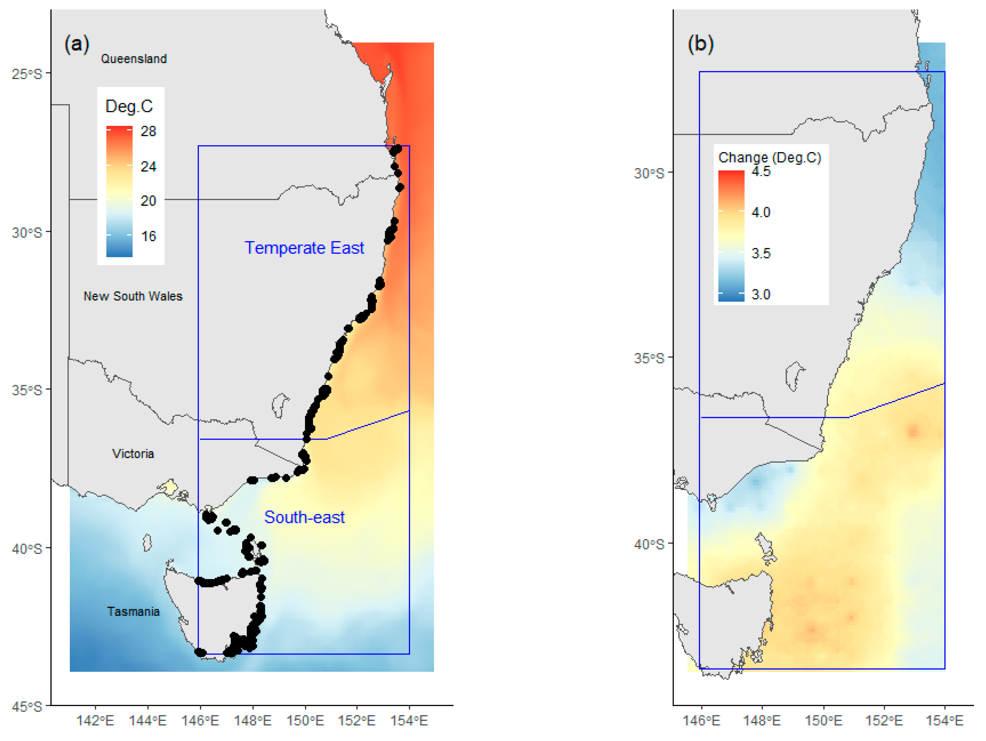
Only data from sites within the geographical bounds where the presence of C. rodgersii had been recorded were included in the modelling, resulting in a study area spanning from southeast Queensland (153.63° E, 27.3° S) to eastern Victoria and Tasmania (145.92° E, 43.36° S, Figure 1a). Data from surveys outside this area were excluded from modelling, as recommended by Zuur et al. [28], to avoid zero inflation through the inclusion of data from regions where C. rodgersii has never been found. Screening resulted in the selection of data from 13,085 standardised surveys at depths ranging between 1 and 40 m. These surveys were undertaken at 573 locations by RLS divers between 2008 and 2022, and at 335 locations by ATRC between 1992 and 2022 [25]. All data were obtained from the Australian Open Data Network (AODN) web portal (portal.aodn.org.au, accessed on 22 November 2022).
2.2. Centrostephanus rodgersii (Urchin) Density Modelling
Centrostephanus rodgersii densities were modelled using a generalised additive mixed effect model (GAMM) framework using a negative binomial distribution. Urchin density data were square-root transformed prior to modelling to reduce skewness. Urchin data were aggregated so that all data from surveys conducted at the same site, in the same month, and in the same depth range (within 5 m) were averaged. Averaging was applied to reduce overfitting models to the data, due to autocorrelation among samples with close spatial and temporal proximities [30]. Models were parameterised using the mgcv package [31] in R [32].
Models were developed using selected explanatory variables of physiological importance to C. rodgersii, with the contributions of each explanatory variable to the model explored through backward stepwise selection; i.e., successively removing individual variables that explained the least amount of variance. The optimal model was selected based on the Akaike information criteria (AIC). The explanatory variables examined were:
- Water temperature at the sampling depth (Tz). Water temperature at depth was selected as a potential explanatory variable, rather than sea surface temperature (SST), as substantial variations in temperature occur with depth within the depth range where urchins are present [16]. Temperature is a key driver of C. rodgersii biological processes, including reproduction and larval survival [33,34]. Water temperatures (Tz) for model development were calculated as the mean of average monthly temperatures in February (i.e., summer maximum) over the period of 2002–2009. Summer temperatures were used as these have been shown to be a more powerful predictor of C. rodgersii densities than annual average temperatures [16]. Water temperatures at sampling depths were extracted from the E.U. Copernicus Marine Service (http://marine.copernicus.eu (accessed on 2 December 2022)), using the Global Ocean Physics Reanalysis monthly mean product (PHY_001_030). Data at the sampling depths were extracted at the closest depth available in the oceanographic re-analysis product;
- Water depth at the sampling site (Depth). Depth was selected as a potential explanatory variable as depth influences a range of factors including pressure, light, and wave exposure and is correlated to C. rodgersii densities [16]. Depth was recorded at each transect;
- Sampling date (Date). Date was included as a potential explanatory variable to allow the investigation of whether changes in C. rodgersii densities occurred over time. Date was incorporated as Julian day numbers throughout the study period;
- Australian marine region (Region). The region was included as a potential explanatory variable to test the hypothesis that changes in C. rodgersii densities over time varied among distinct marine regions. To achieve this, the effects of Date on urchin densities were examined separately in each of the marine regions present. The study area encompassed sections of two distinct marine regions, the Temperate East region and South-east region (Figure 1a), as defined by Richardson et al. [20].
2.3. Historical C. rodgersii Urchin Density Predictions and Climate Change Projections
Following the development of the optimal C. rodgersii density model, historical predictions and future projections of urchin densities were made throughout the study area for three scenarios:
- Predictions for past C. rodgersii densities were made using average summer temperatures at depth (1–40 m), using data from the aforementioned oceanographic reanalysis product for the period 1990–2000;
- Predictions for nominal current C. rodgersii densities were made based on average summer temperatures at depth, using data from the same oceanographic reanalysis product for the period 2010–2020;
- Projections for future C. rodgersii densities, under RCP 8.5, were made using projected future average summer temperature at depth, for the period 2090–2100.
For projections, future temperatures were calculated by adding projected changes to ocean temperatures, between the periods 2002–2009 and 2090–2100, obtained from the Bio-ORACLE model [29] (Figure 1b), to average summer temperature at depth values for the period 2002–2009, from the oceanographic reanalysis product. The use of Bio-ORACLE SST data to derive future summer temperatures at depth was an approximation necessitated by a lack of available future projections for temperatures at depth. This approximation was deemed to be acceptable as future changes to vertical temperature stratification are likely to be small compared to future changes in SST. Furthermore, the addition of ocean temperature change values obtained from the Bio-ORACLE model to historical data from the oceanographic reanalysis produce improves comparability between past, nominal current, and future estimates of C. rodgersii densities.
3. Results
3.1. Reef Life Survey and ATRC Urchin Data
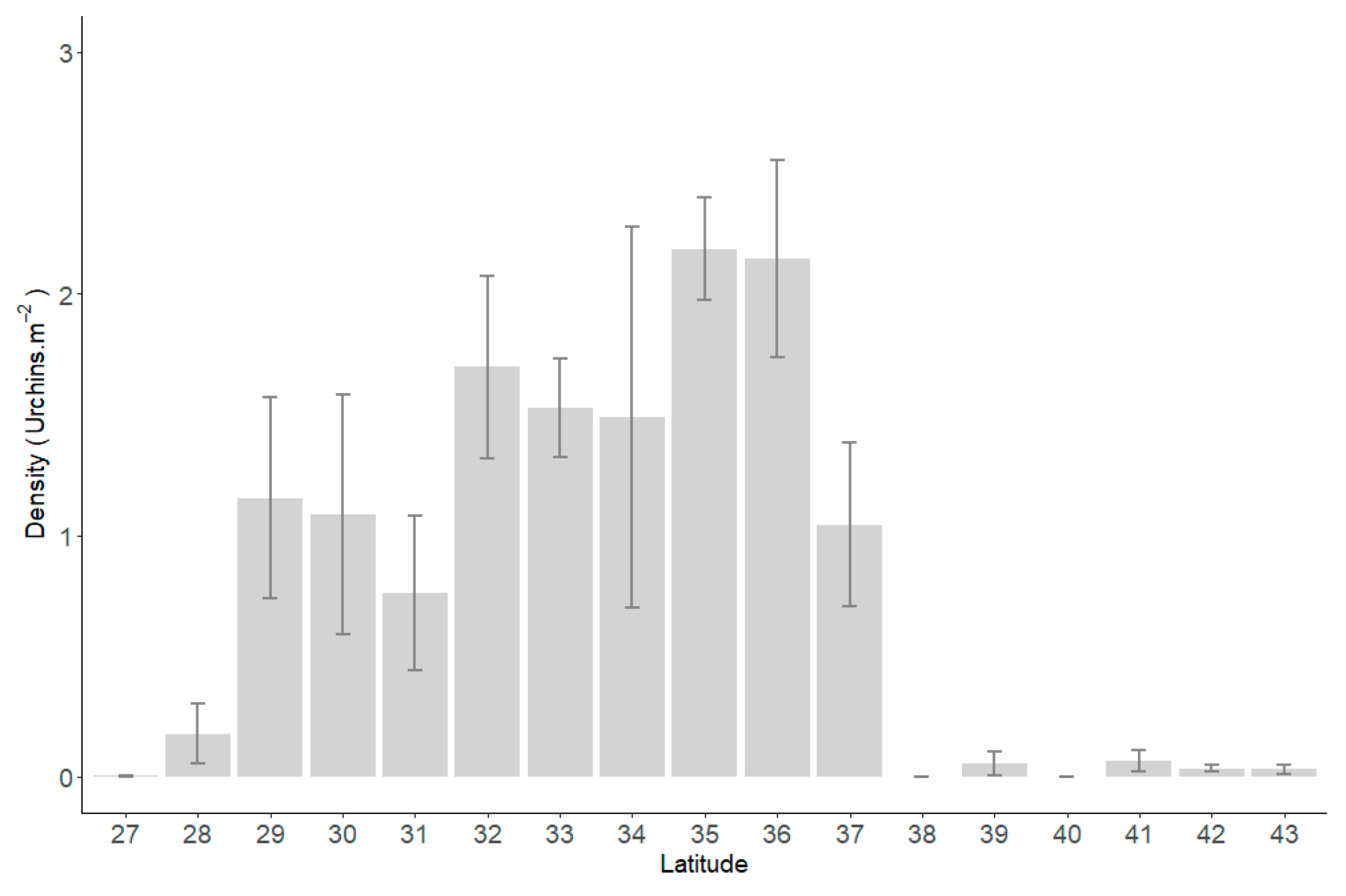
Presences of C. rodgersii were recorded in data from Moreton Bay in Queensland (27.39° S) to the Derwent River in Tasmania (43.35° S, Figure 2). Very low urchin densities were recorded at the northern and southern extremes of this distribution, as was to be expected with these data encompassing the entire realised niche for the species. A maximum density of 24.1 urchins.m−2 was recorded at Jervis Bay (35.05° S) in March 2009, with an average density of 0.89 ± 0.02 urchins.m−2 across the entire current distribution.
3.2. Key Drivers of C. rodgersii Density Variations
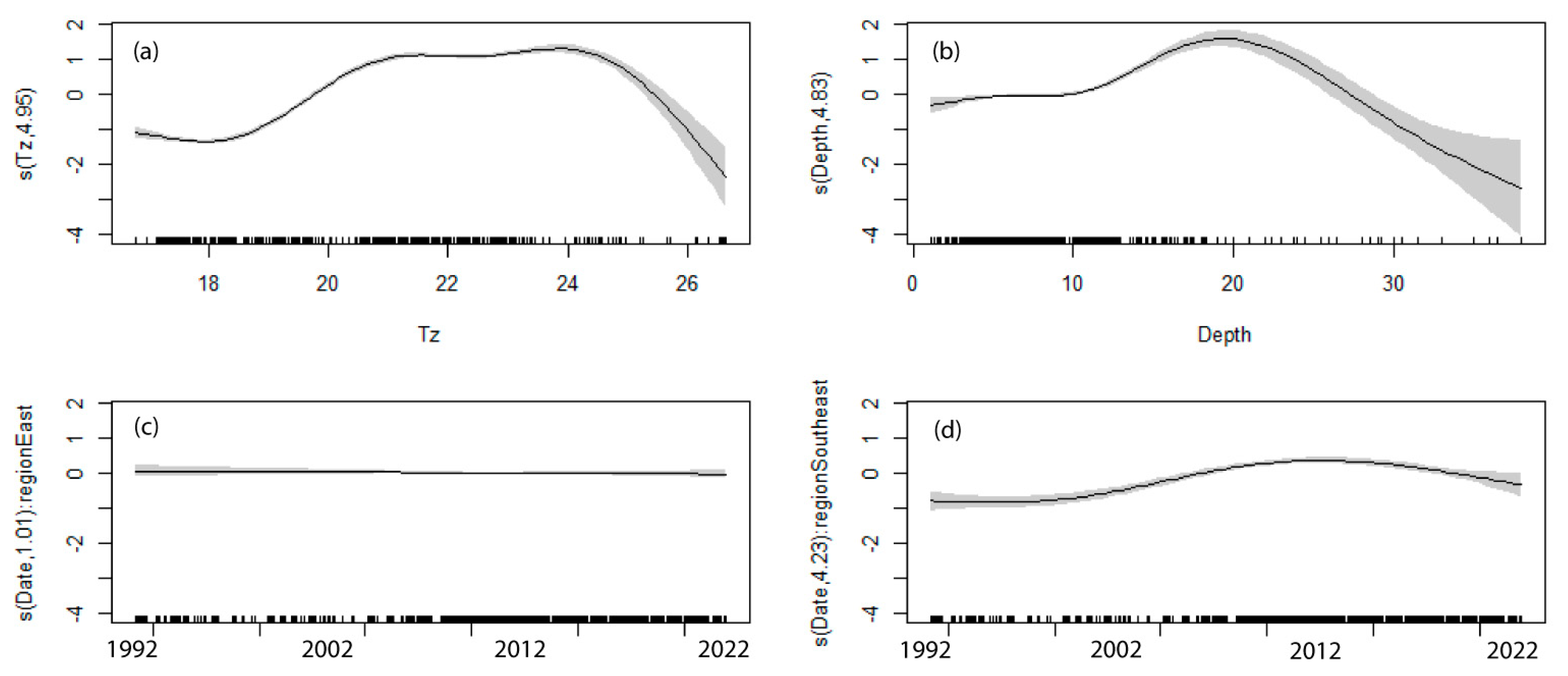
Modelling to determine the significance of factors influencing C. rodgersii densities found that temperature (Tz), Depth, Date and Region were all significant factors in the optimal model developed (i.e., lowest AIC, Table 1). This optimal model explained 44.3% of the variation in urchin densities, with all explanatory variables making significant contributions to the model, although Date only made a significant contribution to the model in the South-east region (Table 2).
Of the explanatory variables, temperature provided the greatest explanatory power, explaining 38.9% of the variation when considered in isolation. The effect of temperature on C. rodgersii densities was non-linear, with low densities occurring at temperatures of 17–19 °C, densities increasing to a plateau from ~21 to 24 °C and densities then rapidly decreasing as temperatures approached 26 °C (Figure 3a). In relation to depth, urchin densities gradually increased with increased depth from 10 to 20 m and then rapidly decreased with depth as this approached 40 m (Figure 3b). Changes over time (as Date) differed between marine regions. In the Temperate East region, there were no significant changes in densities over time (Table 2, Figure 3c). Contrastingly, in the South-east region, there were significant changes over time (Table 2), due to a significant increase in C. rodgersii densities over time (p < 0.001, Figure 3d).
3.3. Predicted and Projected C. rodgersii Densities
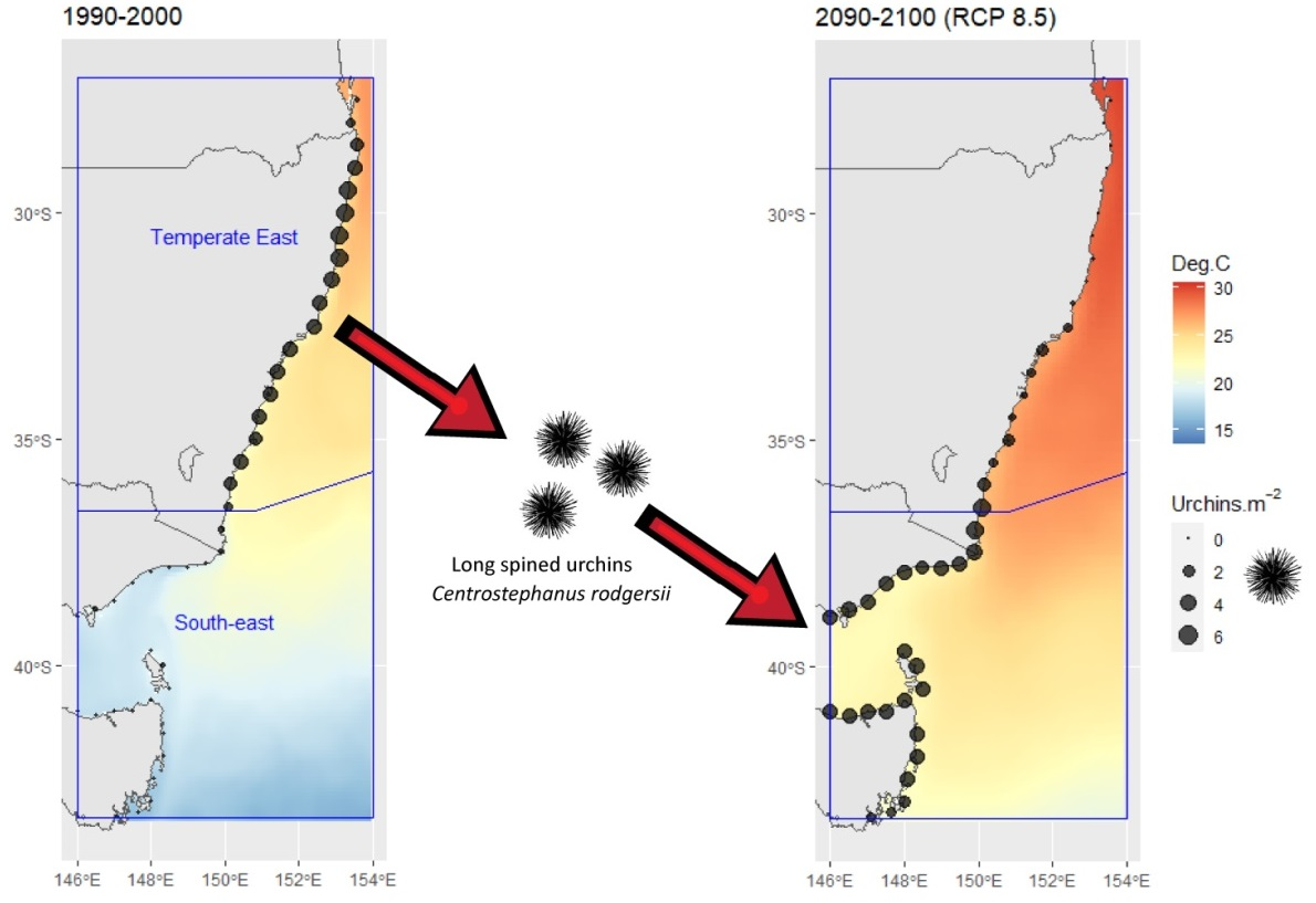
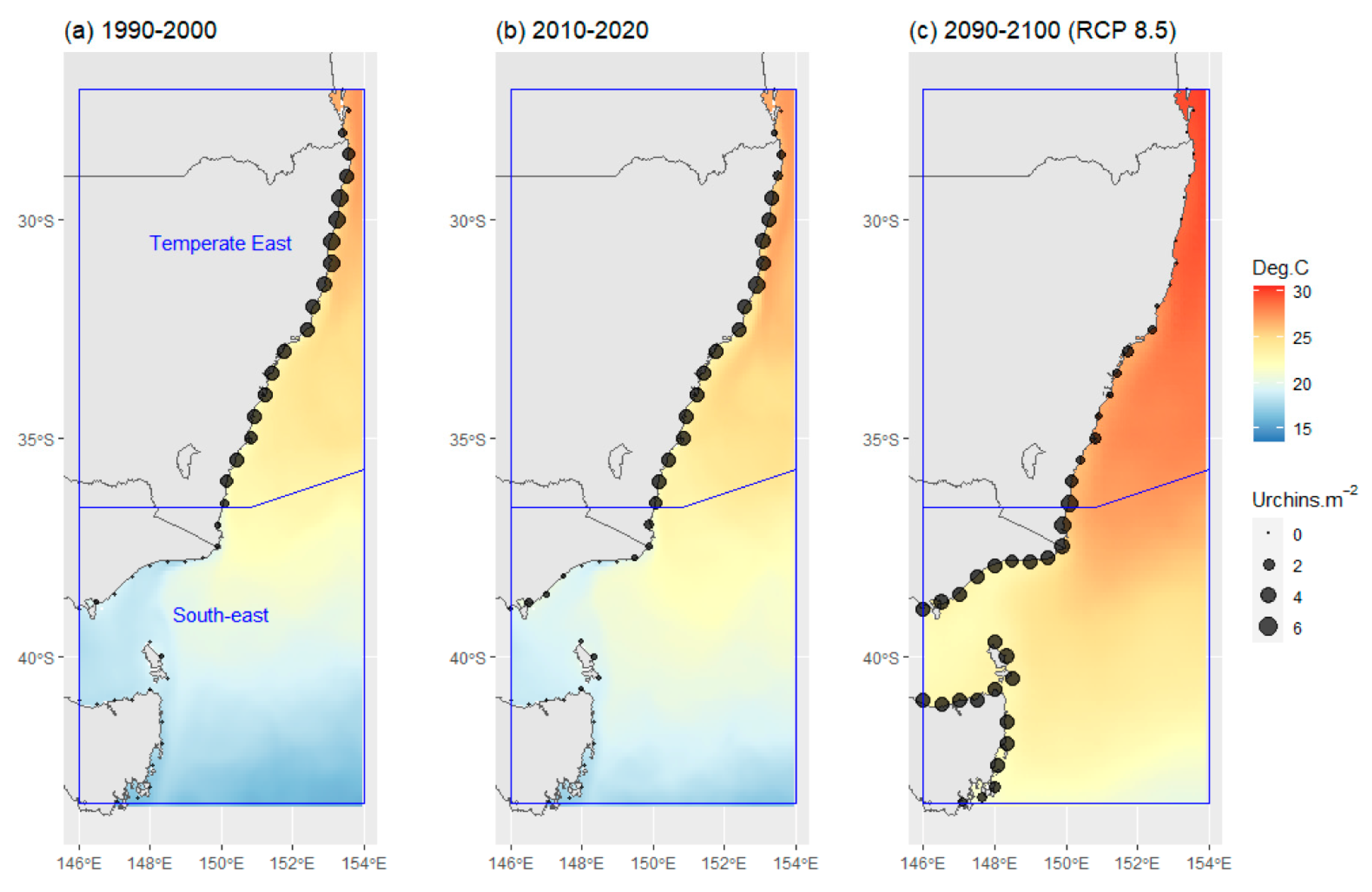
Model predictions for historic C. rodgersii densities, from 1990 to 2000 (Figure 4a) reflect the high abundances of urchins through the Temperate East region (the native range) with low densities into the South-East region. Model predictions for nominal current C. rodgersii densities (2010–2020) reflect the significant increase in densities in the South-east region that has occurred as part of the urchin range expansion (Figure 4b). Simultaneously, predictions indicate declines in C. rodgersii densities in the north of the Temperate East region in 2010–2020, when compared to 1990–2000 (Figure 4a,b).
Application of the model to future projections of C. rodgersii densities (2090–2100), under RCP 8.5, indicated that there could be a dramatic southward shift in the distribution of urchin densities by 2100 (Figure 4c). Large increases in C. rodgersii densities are projected across the South-east region by 2100, with these increases balanced by substantial reductions in urchin densities throughout much of the Temperate East region, particularly at lower latitudes (Figure 4c).
4. Discussion
This study demonstrates that C. rodgersii densities are changing differently in different marine regions in Australia and indicates that densities are not consistently increasing throughout the species’ range. Our results support the hypothesis that ocean warming has driven increases in densities on higher latitude reefs in the South-east region and indicate that warming has not caused substantial changes to C. rodgersii densities in the Temperate East region, although modelling suggests that declines in the north of the Temperate East region may be occurring. Findings are consistent with the previously documented range expansion of C. rodgersii into Tasmania, with significant increases in its abundance occurring in the South-east region [5,19] and with studies from NSW that have identified that C. rodgersii is a stable feature of ecosystems in the Temperate East region [12,35].
Future projections, based on IPCC scenario RCP 8.5, indicate that there will be marked changes in the distribution of C. rodgersii across south-eastern Australia. Substantial shifts in the distributions and densities of C. rodgersii are projected by 2100, with changes expected to differ markedly among regions. Substantial increases in densities are projected in the South-east region, whereas range contractions are projected in the north in the Temperate East region, accompanied by considerable declines in densities across most of the region. Projections for the Temperate East region are generally in agreement with those made by Davis et al. [36], who also projected substantial declines in C. rodgersii densities in NSW by 2100 under RCP8.5. However, Davis et al. [36] projected that these declines would occur throughout NSW, whereas our modelling indicates that declines will be concentrated in northern and central NSW, with increases in C. rodgersii densities possible on the southern NSW coast. The differences between these model projections are most probably due to variations in the geographical and temporal extent and quality of the urchin data used for model construction. The Davis et al. [36] study was based on towed video surveys conducted in NSW in 2020, whereas the current study was based on underwater visual census (UVC) data collected over 30 years across the entire geographical distribution of C. rodgersii in Australia. Therefore, we argue that the current study is likely to provide a more reliable projection of changes, particularly for southern NSW which is at the boundary of the Davis et al. [36] model. Long-term datasets such as the one used in this study are crucial to confidently monitor range shifts and changes in abundance. The early identification and understanding of ecological shifts and the potential issues that may occur then provide the opportunity to tailor appropriate management actions for population conservation or reduction, as required.
It should be noted that future shifts to urchin densities and distributions will be influenced by a range of other unquantified factors, which were not examined in this study. These unquantified factors include physical and hydrological barriers to larval dispersal, changes to ocean mixing and vertical stratification, ocean acidification, and the development of novel ecological interactions. As adult C. rodgersii are relatively immobile, larval dispersal will play a key role in future range expansions [37], with the successful range expansion of immobile marine species dependent on conditions at a new location being suitable for larval settlement and long-term survival, and on the supply of competent larvae [38]. In eastern Australia, the larval supply for C. rodgersii is facilitated by strong poleward flows of the East Australian Current (EAC), which enables the long-range dispersal of pelagic larvae [37], with the EAC linked to the recent range expansion of C. rodgersii into Tasmania [5]. Consequently, the projected future poleward shifts in densities for C. rodgersii are unlikely to be limited by larval dispersal but are more likely to be limited by the prevalence of suitable conditions for larval settlement and persistence.
Modelling identified significant non-linear relationships between C. rodgersii densities and summer bottom water temperatures. Urchin densities were low in locations where summer bottom temperatures were in the range of 17–19 °C, high for locations at 21–24 °C, and low for locations with temperatures > 26 °C. This pattern closely matches the experimentally measured range for successful larval development of C. rodgersii (17.2–24.5 °C) as reported by Pecorino et al. [33] but does not compare as well against the optimal thermal range for C. rodgersii larvae (14.1–21.3 °C), within which, 90% of echinoplutei larvae survived, as determined by Byrne et al. [10]. These differences may reflect varying larval thermal tolerances among northern and southern populations of C. rodgersii. Regardless, the larval development of ectotherms is closely linked to the realised niche of adults [39] and likely imposes constraints on the distribution of C. rodgersii at both high and low latitudes.
The results also revealed a non-linear relationship between C. rodgersii densities and depth, with densities increasing up to depths of ~20 m and then decreasing with depth. This is similar to relationships reported between C. rodgersii densities and depth in NSW, where urchins are generally abundant from 2 to 20 m and then decrease with depth [9,40], whereas, in Tasmania, C. rodgersii generally occur in deeper waters (10–25 m, [9]). Given that declines in C. rodgersii densities are projected in the Temperate East region over the coming decades, deeper and therefore cooler offshore waters have the potential to act as refugia for urchins in this region, with these waters also expected to provide refugia for kelp against warming oceans in this region [16].
5. Conclusions
It was found that C. rodgersii densities are not responding to ocean warming equally across its complete current distributional range in Australia, with densities only found to be increasing significantly in the South-east region. Future projections indicate that increases in C. rodgersii densities in this region will accelerate over the coming decades under the RCP 8.5 climate change scenario. Consequently, the ecological impacts of C. rodgersii, including the formation of barrens, are likely to increase within the South-east region by 2100. The significance of these predicted changes means that potential mitigation strategies will need to be considered, as the increases in urchin abundances are likely to place enormous pressures on kelp habitats in this region, in addition to the pressures already placed on kelp by warming waters. Contrastingly, C. rodgersii densities are projected to decline in the Temperate East region over the same period, with a concomitant reduction in the ecological influence of urchins on ecosystems. In this region, conservation actions to preserve declining C. rodgersii urchin stocks may be required. Our results support other recommendations to consider different management approaches between NSW and other regions [41].
Author Contributions
Conceptualization, T.R.D. and R.P.; Data curation, N.A.K.; Formal analysis, T.R.D. and C.C.; Funding acquisition, R.P.; Investigation, T.R.D. and N.A.K.; Methodology, T.R.D., N.A.K. and C.C.; Project administration, T.R.D.; Software, T.R.D.; Supervision, R.P.; Validation, C.C.; Visualization, T.R.D.; Writing—original draft, T.R.D. and R.P.; Writing—review and editing, N.A.K., C.C. and R.P. All authors have read and agreed to the published version of the manuscript.
Funding
This research was funded by the NSW Marine Estate Management Strategy, Initiative 3.
Institutional Review Board Statement
Not applicable.
Data Availability Statement
Publicly available datasets were analysed in this study. Water temperatures at sampling depths can be extracted from the E.U. Copernicus Marine Service (http://marine.copernicus.eu (accessed on 2 December 2022)). Future temperature projections can be extracted from the Bio-ORACLE portal at: https://www.bio-oracle.org (accessed on 15 December 2022). RLS and ATRC survey data can be obtained from the Australian Open Data Network (AODN) web portal at: http://portal.aodn.org.au (accessed on 22 November 2022).
Acknowledgments
We thank the enormous number of volunteer RLS divers and scientists (RLS and ATRC) who have collected data over large spatial scales and long periods of time—especially Graham Edgar, Neville Barrett, Rick Stuart-Smith, Toni Cooper, and Lizzie Oh. Thanks also to Rowan Chick for his valuable feedback which greatly improved the final manuscript. Data were sourced from Australia’s Integrated Marine Observing System (IMOS)—IMOS is enabled by the National Collaborative Research Infrastructure Strategy (NCRIS).
Conflicts of Interest
The authors declare no conflict of interest. The funders had no role in the design of the study; in the collection, analyses, or interpretation of data; in the writing of the manuscript; or in the decision to publish the results.
References
- Doney, S.C.; Ruckelshaus, M.; Emmett Duffy, J.; Barry, J.P.; Chan, F.; English, C.A.; Galindo, H.M.; Grebmeier, J.M.; Hollowed, A.B.; Knowlton, N. Climate Change Impacts on Marine Ecosystems. Ann. Rev. Mar. Sci. 2012, 4, 11–37. [Google Scholar] [CrossRef] [Green Version]
- Babcock, R.C.; Bustamante, R.H.; Fulton, E.A.; Fulton, D.J.; Haywood, M.D.E.; Hobday, A.J.; Kenyon, R.; Matear, R.J.; Plaganyi, E.E.; Richardson, A.J. Severe Continental-Scale Impacts of Climate Change Are Happening Now: Extreme Climate Events Impact Marine Habitat Forming Communities along 45% of Australia’s Coast. Front. Mar. Sci. 2019, 6, 411. [Google Scholar] [CrossRef]
- Filbee-Dexter, K.; Scheibling, R.E. Sea Urchin Barrens as Alternative Stable States of Collapsed Kelp Ecosystems. Mar. Ecol. Prog. Ser. 2014, 495, 1–25. [Google Scholar] [CrossRef] [Green Version]
- Steneck, R.S.; Graham, M.H.; Bourque, B.J.; Corbett, D.; Erlandson, J.M.; Estes, J.A.; Tegner, M.J. Kelp Forest Ecosystems: Biodiversity, Stability, Resilience and Future. Environ. Conserv. 2002, 29, 436–459. [Google Scholar] [CrossRef] [Green Version]
- Ling, S.D. Range Expansion of a Habitat-Modifying Species Leads to Loss of Taxonomic Diversity: A New and Impoverished Reef State. Oecologia 2008, 156, 883–894. [Google Scholar] [CrossRef] [PubMed]
- Thomas, L.J.; Liggins, L.; Banks, S.C.; Beheregaray, L.B.; Liddy, M.; McCulloch, G.A.; Waters, J.M.; Carter, L.; Byrne, M.; Cumming, R.A. The Population Genetic Structure of the Urchin Centrostephanus Rodgersii in New Zealand with Links to Australia. Mar. Biol. 2021, 168, 138. [Google Scholar] [CrossRef]
- Andrew, N.L. Spatial Heterogeneity, Sea Urchin Grazing, and Habitat Structure on Reefs in Temperate Australia. Ecology 1993, 74, 292–302. [Google Scholar] [CrossRef]
- Fletcher, W.J. Interactions among Subtidal Australian Sea Urchins, Gastropods, and Algae: Effects of Experimental Removals. Ecol. Monogr. 1987, 57, 89–109. [Google Scholar] [CrossRef]
- Byrne, M.; Andrew, N.L. Centrostephanus Rodgersii and Centrostephanus Tenuispinus. Dev. Aquac. Fish. Sci. 2020, 43, 379–396. [Google Scholar]
- Byrne, M.; Gall, M.L.; Campbell, H.; Lamare, M.D.; Holmes, S.P. Staying in Place and Moving in Space: Contrasting Larval Thermal Sensitivity Explains Distributional Changes of Sympatric Sea Urchin Species to Habitat Warming. Glob. Chang. Biol. 2022, 28, 3040–3053. [Google Scholar] [CrossRef]
- Johnson, C.R.; Ling, S.D.; Ross, D.J.; Shepherd, S.; Miller, K.J. Establishment of the Long-Spined Sea Urchin (Centrostephanus Rodgersii) in Tasmania: First Assessment of Potential Threats to Fisheries; School of Zoology and Tasmanian Aquaculture and Fisheries Institute: Hobart, Australia, 2005. [Google Scholar]
- Glasby, T.M.; Gibson, P.T. Decadal Dynamics of Subtidal Barrens Habitat. Mar. Environ. Res. 2020, 154, 104869. [Google Scholar] [CrossRef] [PubMed]
- Underwood, A.J.; Kingsford, M.J.; Andrew, N.L. Patterns in Shallow Subtidal Marine Assemblages along the Coast of New South Wales. Aust. J. Ecol. 1991, 16, 231–249. [Google Scholar] [CrossRef]
- Andrew, N.L.; Underwood, A.J. Associations and Abundance of Sea Urchins and Abalone on Shallow Subtidal Reefs in Southern New South Wales. Mar. Freshw. Res. 1992, 43, 1547–1559. [Google Scholar] [CrossRef]
- Davis, T.R.; Cadiou, G.; Champion, C.; Coleman, M.A. Environmental Drivers and Indicators of Change in Habitat and Fish Assemblages within a Climate Change Hotspot. Reg. Stud. Mar. Sci. 2020, 36, 101295. [Google Scholar] [CrossRef]
- Davis, T.R.; Champion, C.; Coleman, M.A. Climate Refugia for Kelp within an Ocean Warming Hotspot Revealed by Stacked Species Distribution Modelling. Mar. Environ. Res. 2021, 166, 105267. [Google Scholar] [CrossRef]
- Andrew, N.L.; Underwood, A.J. Patterns of Abundance of the Sea Urchin Centrostephanus Rodgersii (Agassiz) on the Central Coast of New South Wales, Australia. J. Exp. Mar. Biol. Ecol. 1989, 131, 61–80. [Google Scholar] [CrossRef]
- Andrew, N.L. Changes in Subtidal Habitat Following Mass Mortality of Sea Urchins in Botany Bay, New South Wales. Aust. J. Ecol. 1991, 16, 353–362. [Google Scholar] [CrossRef]
- Keane, J.P.; Ling, S.D. Range Extension of the Long Spined Sea Urchin-Centrostephanus Rodgersii. In Proceedings of the SE Australia MCIA Symposium, CSIRO, Hobart, Australia, 20–21 February 2018. [Google Scholar]
- Richardson, A.J.; Eriksen, R.; Moltmann, T.; Hodgson-Johnston, I.; Wallis, J.R. State and Trends of Australia’s Ocean Report; Integrated Marine Observing System: Hobart, Australia, 2020. [Google Scholar]
- Duran, E.R.; England, M.H.; Spence, P. Surface Ocean Warming around Australia Driven by Interannual Variability and Long-term Trends in Southern Hemisphere Westerlies. Geophys. Res. Lett. 2020, 47, e2019GL086605. [Google Scholar] [CrossRef]
- IPCC. Climate Change 2014: Synthesis Report. In Contribution of Working Groups I, II and III to the Fifth Assessment Report of the Intergovernmental Panel on Climate Change; IPCC: Geneva, Switzerland, 2014. [Google Scholar]
- Schwalm, C.R.; Glendon, S.; Duffy, P.B. RCP8. 5 Tracks Cumulative CO2 Emissions. Proc. Natl. Acad. Sci. USA 2020, 117, 19656–19657. [Google Scholar] [CrossRef]
- Edgar, G.J.; Cooper, A.; Baker, S.C.; Barker, W.; Barrett, N.S.; Becerro, M.A.; Bates, A.E.; Brock, D.; Ceccarelli, D.M.; Clausius, E. Reef Life Survey: Establishing the Ecological Basis for Conservation of Shallow Marine Life. Biol. Conserv. 2020, 252, 108855. [Google Scholar] [CrossRef]
- Edgar, G.J.; Barrett, N.S. Short Term Monitoring of Biotic Change in Tasmanian Marine Reserves. J. Exp. Mar. Biol. Ecol. 1997, 213, 261–279. [Google Scholar] [CrossRef]
- Edgar, G.J.; Stuart-Smith, R.D. Ecological Effects of Marine Protected Areas on Rocky Reef Communities-a Continental-Scale Analysis. Mar. Ecol. Prog. Ser. 2009, 388, 51–62. [Google Scholar] [CrossRef]
- Edgar, G.J.; Stuart-Smith, R.D. Systematic Global Assessment of Reef Fish Communities by the Reef Life Survey Program. Sci. Data 2014, 1, 140007. [Google Scholar] [CrossRef] [PubMed] [Green Version]
- Zuur, A.F.; Saveliev, A.A.; Leno, E.N. Zero Inflated Models and Generalized Linear Mixed Models with R; Highland Statistics Ltd.: Newburgh, UK, 2012; ISBN 0957174101. [Google Scholar]
- Tyberghein, L.; Verbruggen, H.; Pauly, K.; Troupin, C.; Mineur, F.; de Clerck, O. Bio-ORACLE: A Global Environmental Dataset for Marine Species Distribution Modelling. Glob. Ecol. Biogeogr. 2012, 21, 272–281. [Google Scholar] [CrossRef]
- Johnston, A.; Hochachka, W.; Strimas-Mackey, M.; Gutierrez, V.R.; Robinson, O.; Miller, E.; Auer, T.; Kelling, S.; Fink, D. Best Practices for Making Reliable Inferences from Citizen Science Data: Case Study Using EBird to Estimate Species Distributions. BioRxiv 2019, 574392, 1–13. [Google Scholar]
- Wood, S.N. Fast Stable Restricted Maximum Likelihood and Marginal Likelihood Estimation of Semiparametric Generalized Linear Models. J. R. Stat. Soc. Ser. B Stat. Methodol. 2011, 73, 3–36. [Google Scholar] [CrossRef] [Green Version]
- R Core Team. R: A Language and Environment for Statistical Computing; R Foundation for Statistical Computing: Vienna, Austria, 2022. [Google Scholar]
- Pecorino, D.; Lamare, M.D.; Barker, M.F.; Byrne, M. How Does Embryonic and Larval Thermal Tolerance Contribute to the Distribution of the Sea Urchin Centrostephanus Rodgersii (Diadematidae) in New Zealand? J. Exp. Mar. Biol. Ecol. 2013, 445, 120–128. [Google Scholar] [CrossRef]
- Byrne, M.; Andrew, N.L.; Worthington, D.G.; Brett, P.A. Reproduction in the Diadematoid Sea Urchin Centrostephanus Rodgersii in Contrasting Habitats along the Coast of New South Wales, Australia. Mar. Biol. 1998, 132, 305–318. [Google Scholar] [CrossRef]
- Hill, N.A.; Blount, C.; Poore, A.G.B.; Worthington, D.; Steinberg, P.D. Grazing Effects of the Sea Urchin Centrostephanus Rodgersii in Two Contrasting Rocky Reef Habitats: Effects of Urchin Density and Its Implications for the Fishery. Mar. Freshw. Res. 2003, 54, 691–700. [Google Scholar] [CrossRef]
- Davis, T.R.; Champion, C.; Coleman, M.A. Ecological Interactions Mediate Projected Loss of Kelp Biomass under Climate Change. Divers. Distrib. 2022, 28, 306–317. [Google Scholar] [CrossRef]
- Banks, S.C.; Piggott, M.P.; Williamson, J.E.; Bové, U.; Holbrook, N.J.; Beheregaray, L.B. Oceanic Variability and Coastal Topography Shape Genetic Structure in a Long-dispersing Sea Urchin. Ecology 2007, 88, 3055–3064. [Google Scholar] [CrossRef] [PubMed] [Green Version]
- Abrego, D.; Howells, E.J.; Smith, S.D.A.; Madin, J.S.; Sommer, B.; Schmidt-Roach, S.; Cumbo, V.R.; Thomson, D.P.; Rosser, N.L.; Baird, A.H. Factors Limiting the Range Extension of Corals into High-Latitude Reef Regions. Diversity 2021, 13, 632. [Google Scholar] [CrossRef]
- Collin, R.; Rebolledo, A.P.; Smith, E.; Chan, K.Y.K. Thermal Tolerance of Early Development Predicts the Realized Thermal Niche in Marine Ectotherms. Funct. Ecol. 2021, 35, 1679–1692. [Google Scholar] [CrossRef]
- Andrew, N. Under Southern Seas: The Ecology of Australia’s Rocky Reefs; UNSW Press: Sydney, Australia, 1999; ISBN 0868406570. [Google Scholar]
- Kingsford, M.; Byrne, M. NSW Rocky Reefs Are under Threat. Mar. Freshw. Res. 2023, in press. [Google Scholar] [CrossRef]
Figure 1.
(a) Study area in Australia separated into marine regions (blue rectangles) showing (a) sampling locations (dots) and average February (i.e., summer) water temperature (2002–2009) at a depth of 0.5m. (b) Projected change in sea surface temperatures by 2100 under RCP 8.5. Future temperature data are from the Bio-ORACLE model [29].

Figure 2.
Average density of Centrostephanus rodgersii urchins on Reef Life Survey transects for one-degree latitudinal bins eastern Australia. Averaging conducted for all sites in each bin, across all survey dates (1992–2022) and depths (1–40 m). Error bars ± Standard Error.
Figure 2.
Average density of Centrostephanus rodgersii urchins on Reef Life Survey transects for one-degree latitudinal bins eastern Australia. Averaging conducted for all sites in each bin, across all survey dates (1992–2022) and depths (1–40 m). Error bars ± Standard Error.

Figure 3.
Effects of explanatory variables on C. rodgersii urchin densities for the optimal explanatory model developed for Australia. Solid lines show average predicted values with shaded areas showing standard errors and small vertical marks along the x-axis show data points. (a) Effect of summer water temperature at depth (Tz), (b) effect of depth, (c) effect of survey date in Temperate East region, and (d) effect of survey date in South-east region.

Figure 4.
Centrostephanus rodgersii urchin density predictions and projections made using the optimal explanatory model developed for Australia. (a) Predictions for average densities from 1990 to 2000, (b) predictions for average densities from 2010 to 2020, (c) projections for average densities under climate change scenario RCP 8.5 for the period 2090–2100. Contours show average summer maximum (February) temperatures for the reference period. Blue boxes indicate distinct marine regions in Australia as shown in Figure 1a [20].


Table 1.
Backward stepwise selection of explanatory variables for models to explain C. rodgersii urchin densities at sites in Australia. Tz = average from 2002 to 2009 of the summer monthly (February) temperature at depth (z). Depth = average survey depth (m). Date:Region = survey date by region (East, South-east).
| Model | Variables | AIC | ΔAIC | Deviance Explained |
|---|---|---|---|---|
| 1 | Date:Region + Depth + Tz | 20,276.8 | 0.0 | 44.3% |
| 2 | Depth + Tz | 20,436.9 | 160.1 | 42.2% |
| 3 | Tz | 20,704.1 | 427.3 | 38.9% |
Table 2.
Contribution of variables to the optimal model for describing C. rodgersii urchin density variations across sites in Australia. Tz = average from 2002 to 2009 of the summer monthly (February) temperature at depth (z). Depth = average survey depth (m). Date:Region = survey date by region (Temperate East, South-east).
| Variables | Effective Degrees of Freedom | p-Value |
|---|---|---|
| Tz | 4.948 | <0.001 |
| Depth | 4.828 | <0.001 |
| Date:Region (Temperate East) | 1.012 | 0.496 |
| Date:Region (South-east) | 4.234 | <0.001 |
Disclaimer/Publisher’s Note: The statements, opinions and data contained in all publications are solely those of the individual author(s) and contributor(s) and not of MDPI and/or the editor(s). MDPI and/or the editor(s) disclaim responsibility for any injury to people or property resulting from any ideas, methods, instructions or products referred to in the content. |
© 2023 by the authors. Licensee MDPI, Basel, Switzerland. This article is an open access article distributed under the terms and conditions of the Creative Commons Attribution (CC BY) license (https://creativecommons.org/licenses/by/4.0/).
Share and Cite
MDPI and ACS Style
Davis, T.R.; Knott, N.A.; Champion, C.; Przeslawski, R. Impacts of Climate Change on Densities of the Urchin Centrostephanus rodgersii Vary among Marine Regions in Eastern Australia. Diversity 2023, 15, 419. https://doi.org/10.3390/d15030419
AMA Style
Davis TR, Knott NA, Champion C, Przeslawski R. Impacts of Climate Change on Densities of the Urchin Centrostephanus rodgersii Vary among Marine Regions in Eastern Australia. Diversity. 2023; 15(3):419. https://doi.org/10.3390/d15030419
Chicago/Turabian StyleDavis, Tom R., Nathan A. Knott, Curtis Champion, and Rachel Przeslawski. 2023. "Impacts of Climate Change on Densities of the Urchin Centrostephanus rodgersii Vary among Marine Regions in Eastern Australia" Diversity 15, no. 3: 419. https://doi.org/10.3390/d15030419
Note that from the first issue of 2016, this journal uses article numbers instead of page numbers. See further details here.