Article

Species Abundance Distributions Patterns between Tiankeng Forests and Nearby Non-Tiankeng Forests in Southwest China

1
Key Laboratory of Ecology of Rare and Endangered Species and Environmental Protection (Ministry of Education), Guangxi Normal University, Guilin 541004, China
2
Guangxi Key Laboratory of Landscape Resources Conservation and Sustainable Utilization in Lijiang River Basin, Guangxi Normal University, Guilin 541004, China
3
College of Life Sciences, Guangxi Normal University, Guilin 541004, China
*
Author to whom correspondence should be addressed.
These authors contributed equally to this work.
Diversity 2022, 14(2), 64; https://doi.org/10.3390/d14020064
Submission received: 28 November 2021 / Revised: 10 January 2022 / Accepted: 12 January 2022 / Published: 19 January 2022
(This article belongs to the Special Issue Ecology, Evolution and Diversity of Plants)

Abstract

:
Identifying the species abundance distributions (SADs) in Tiankeng forests is crucial for restoring and managing degraded karst ecosystem, whereas previous studies rarely explored the differences and response of vegetation dynamics to environmental variations. The species composition and SADs of the inner and outer fringe areas of Tiankeng forest and nearby non-Tiankeng forest were compared in Southwest China. Six models were adopted to compare SADs of three habitats. Kolmogrov–Smirnov (K–S) test was selected to compare the discrepancy between the simulated and observed SAD patterns. The Akaike Information Criterion (AIC) test was adopted to compare the models, and the best model was indicated by the lowest AIC value. The results showed that (1) the species dispersal from the inside of Tiankeng forests to the nearby non-Tiankeng forests is limited, while species have unlimited dispersal from nearby non-Tiankeng forests to the inside of Tiankeng forests via the fringe of Tiankeng forests. (2) Species abundance, species rarity, richness, and species accumulation rate in the Tiankeng forests were significant in non-Tiankeng forests (p < 0.05), and most species in inner Tiankeng forests originated from nearby non-Tiankeng forests. (3) Based on the criterion of K-S values, all models have passed the K–S test (p > 0.05), which indicated that niche processes and neutral process worked together in the maintenance of community species diversity, the community in study area is a niche-neutral continuum. (4) Considered the lowest AIC value, the neutral (△mean AIC = 1.3) models performed better than the niche (△mean AIC = 22.7) models and statistical (△mean AIC = 2.7) in the Tiankeng forest, while the statistical models performed better than the niche and neutral models in the non-Tiankeng forests. The results suggested that the main driving force of Tiankeng forests is the neutral process. The negative terrain in Tiankeng restricted the species dispersal due to topographic constraints. However, the species dispersal from the nearby non-Tiankeng forests could promote the species succession in the inner Tiankeng. Therefore, we propose that nearby non-Tiankeng forests should be emphasized for protecting the biodiversity of Tiankeng forests.

1. Introduction

Understanding the mechanism for the maintenance of species diversity in communities has become an issue of ecological concern [1]. At present, two major theories have been advanced to explain the rules of community assembly mechanisms. Niche theory proposes that species diversity is affected by deterministic processes, such as environment filtering, competition, and exclusion within species [2,3,4], while neutral theory emphasizes the effect of random processes, such as diffusion limitation on the composition and distribution of species, distance decay, and species turnover rate [5,6,7]. Species abundance distribution (SAD), the basic proportional abundance of species combined in an ecological community, is one of the important ways to encapsulate the characteristics of community diversity [8,9].
Since the 1940s, all kinds of models have been used to verify mechanistic rules to explain the structure of ecological communities, and reveal the effects of various ecological processes in SADs patterns [10,11]. There are three types of models, namely statistical, niche, and neutral. Statistical models, such as Fisher’s log-series and Preston log-normal, describe the complexity of community composition using mathematics [12,13]. Niche models, such as the Broken stick and Niche preemption, focus on the connection of niche theory and SAD to infer species competition or repulsion [14,15,16]. While the neutral models, such as Zero-sum polynomials [16,17] and Volkov model [18], are used in testing for random species abundance patterns and emphasizing random effects on community construction [8]. Different models can only demonstrate a part of community ecological process. Therefore, many scholars mostly adopt a combination of multiple models to analyze the SAD pattern in different objects, including alpine meadows [19], tropical forests [20], subtropical evergreen-deciduous broadleaved mixed forests [21]. However, the current research on forest communities of SAD models in negative terrain habitats is still unclear.
Tiankeng is a kind of karst negative terrain with a huge volume [22,23]. The Tiankeng forest is located in the Tiankeng. The Tiankeng forest is divided into two areas and each have their own unique features. At the top of Tiankeng is the fringe area, a complex ecotone between the nearby non-Tiankeng forest and Tiankeng forests was influenced by some human disturbance. The Tiankeng forest interior is located on the negative terrain of the Tiankeng and is surrounded by the fringe of Tiankeng forest. Here, the topography is steeped and sloped, and there are adequate hydrothermal conditions and less human interference [23,24]. The nearby non-Tiankeng forest, located in a positive terrain, is a well-preserved karst forest near Tiankeng [25,26,27]. From an existing vegetation distribution perspective, the non-Tiankeng forest vegetation reflects the adaptation of species to limestone geology and human disturbance, while the Tiankeng forest reflects species independent evolution in a natural negative terrain [27,28]. At present, most studies on Tiankeng forests focus on geological features [29], landscape value [22], biodiversity [24], plant community structure [23], interspecific association [30], functional traits, and species adaption to the environment [25]. However, only a few studies have focused on the effects of nearby non-Tiankeng forests, especially for the species dispersal or invasion [24,27].
The Tiankeng and nearby non-Tiankeng forests are unique vegetation distributed on karst landforms. Combining the SADs pattern in Tiankeng forests and nearby non-Tiankeng forests not only benefits us to reveal the maintenance mechanism of species diversity in fragmented forests, but also helps us to suggest vegetation restoration and reconstruction in ecologically sensitive areas. In this study, we selected three habitats, the inside of Tiankeng forests, the fringe of Tiankeng forests and the nearby non-Tiankeng forests as the study area A total of six sampling plots were established at a scale of 40 m × 40 m. Based on the composition characteristics of woody plant, the variations in important value of dominant species, species empirical cumulative distribution functions (ECDF) curve, species-abundance curve, Jaccard similarity index, and six SAD’s models fitting (Fisher’s log-series, Preston log-normal, Broken stick, Niche preemption, Zero-sum polynomial, and Volkov model) have been utilized to address the following questions for three habitats (the inside of Tiankeng forests, the fringe of Tiankeng forests, and the nearby non-Tiankeng forests): (1) What are their difference in species composition; (2) What are their SADs patterns; (3) What are their main driving forces for the maintenance of community diversity?

2. Materials and Methods

2.1. Study Area

This study was carried out in the Dashiwei Tiankeng Group branch, located at 24°30′ N to 25°03′ N and 106°10′ E to 106°51′ E, in Leye, Guangxi, southwest China. The study area has a big difference in elevation, higher in the southwest (Guizhou plateau) and lower in east, north, and west (Guangxi basin). The local climate is mid-subtropical monsoon. There is a rainy season from May to October. The annual average rainfall is 1400mm, rainfall accounts for 85% of the mean precipitation, annual relative humidity is 85%, and mean average temperature is 16.6–23.0 °C. Hydrological conditions are superior, with the first-level tributary of the Hongshui river–Bailang underground river system. In the middle of the “S”-shaped fold of the Bailang underground river, the river channels are intricate and unique, forming many special peak clusters, depressions, and Tiankeng negative terrain. Soils are developed from limestone weathering and are alkaline acidic clay. The Tiankeng forest was distributed mainly on the Tiankeng negative terrain. The study area is evergreen and deciduous broad-leaved mixed forest with average altitude of 1200~1266 m [22,23,24,25,27].

2.2. Survey and Sampling

To explore SADs between Tiankeng and nearby non-Tiankeng forest, a reconnaissance survey and vegetation data collection in Dashiwei Tiankeng Group was carried out from 10 August to 20 November 2019. Because most of the Tiankeng forests are steep and difficult to reach, the number of plots in each area was determined by the size of forests, community structure, vegetation, and topography conditions [25]. Sampling methods followed Ma [8] and Zhang [31]. Three habitat types (the inside of Tiankeng forest, the fringe of Tiankeng forest, and the nearby non-Tiankeng forest) from six sampling sites were selected within the study area based on differences in location of phytocoenoses in Tiankeng. Furthermore, the study area for each type of habitat was 3200 m2, and each sampling site was divided into 16 plots at a scale of 10 m × 10 m.
The inside of Tiankeng forest includes Liuxing Tiankeng (LX) and Dacao Tiankeng (DC). Liuxing Tiankeng is of 890 m × 320 m and a depth of 210–290 m, which is the second largest Tiankeng in the Dashiwei group, and Dacao Tiankeng is a general Tiankeng of 250 m × 140 m with a depth of 62–108 m. In the inner area of both Tiankengs are reachable, natural, and contain abundant species [22]. The fringe of Tiankeng forest contains the Luojia (LJ) and Shenmu Tiankeng (SM). The Luojia Tiankeng is 140 m × 100 m and 71–128 m deep, and Shenmu Tiankeng is 300 m × 270 m with a depth of 186–234 m. Between Luojia and Shenmu Tiankeng of the outer fringe area, there is human interference and rich species diversity [22]. The nearby non-Tiankeng also includes two sampling sites, one (LA) is near the village and other one (SW) is near the farmland; between them are well protected karst forests with complex communities. For our research, plot names are coded firstly by location (see above), and secondly as either inside of Tiankeng forest (-TK), in the fringe of Tiankeng forest (-BY), or the nearby karst non-Tiankeng forest (-FS) (Figure 1). In each quadrat, the abundance, diameter at breast height, basal diameter, and cover of all woody species with a diameter at breast height ≥1 cm were recorded.

2.3. Data Analysis

All the original data were recorded and preserved in the key laboratory of ecology of rare endangered species and environmental protection, Guangxi Normal University, in order to preliminarily identify the plant scientific names [31]. Plant family, genus, and species were identified by the online Flora of China (http://www.iplant.cn/foc/, accessed on 9 December 2021) and Wei et al. [32] for all the collected specimens. Species abundance comes from the number of individuals of each species recorded in each sampling site. The dominant species were determined by the higher importance value (P) [33]. Species importance value was calculated from the relative frequency (RF), relative abundance (RA), and relative dominance (RD) [34] as:
P = [(RF + RA + RD)/3] × 100%
We used two curves (species ECDF and species abundance curve) to visually observe the SADs pattern in six sampling sites, and a Kruskal–Wallis test (K–W) was used to compare the SAD’s difference in the ‘dplyr’ packages of R software 4.0.0. (R Core Team, Vienna, Austria) [35,36].
The alpha diversity indices, such as species richness (Sp) and Shannon–Wiener index (H′) were assessed for the species, the formula [37] is as follows:
SP = S
H′ = −∑ PilnPi
where S represents the number of species and Pi represents the ratio of the abundance of the i-th species to the total abundance.
The beta diversity indices, such as Jaccard index (C′), were assessed for the species to compare the similarity in two communities. The formula [38] is as follows:
C′ = c/(a + bc)
where a and b are the number of species in the two communities and c is the number of species in common in the two communities.

2.4. Models Selection

Six models were selected to simulate the SAD pattern, including two statistical models (Fisher’s log-series model and Log-normal model), two neutral models (Zero-sum polynomials model and Volkov model), and two niche models (Niche preemption model and Broken stick model) [1,8]. The details are as follows.
(1)
Fisher’s log-series model
This model was proposed by Fisher et al. [39]. It uses a negative binomial distribution to describe the relationship between the number of species and the individuals of species. This model excludes species without individual numbers [40]. The calculation formula [39] is as follows:
S(n) = αXn/n
where α (α > 0) is the species diversity index of the community, similar to species richness, n is species abundance, S is the number of species, and X is a constant (Tends to 1) [16].
(2)
Log-normal model
This model assumes that the logarithm of the number of species in the community conforms to the normal distribution, and the abundance of the i-th species is recorded as Ai. The calculation formula [13] is as follows:
Ai = elog(μ)+log(φ), i = 1,2,3, …, S.
where μ is the mean of the normal distribution, δ is the standard deviation of the normal distribution, and φ is the normal deviation.
(3)
Broken stick model
In this model, a broken stick with a length of 1 is represented as the total niche in the community, and it is given to S species [14]. The competitiveness and taxonomic status of each species are basically similar, and they exist in the community at the same time [15]. If the total number of individuals in the community is J, the abundance Ai of the i-th species is:
Ai = J/S, i = 1,2,3, …, S.
(4)
Niche preemption model
The model assumes that species 1 first occupies k parts of the niche in the community, and species 2 occupies the remaining k(1 − k)2 parts, and so on, until the remaining resources cannot sustain the survival of another species [15]. If A1 is the abundance of the most dominant species predicted by the model, the abundance Ai of the i-th species is:
Ai = A1 (1k)i−1, i = 1,2,3, …, S.
(5)
Zero-sum polynomials model
This model assumes that the species abundance distribution at a certain point is derived from the random drift of the neutral composite community. This model includes two parameters, the number of individual species (J) at the sampling point and the fundamental biodiversity number (θ) [17]. Therefore, the number S of species with an abundance of n at a sampling point in the composite community is expressed by the formula:
S(n) = 0Jfn,i(y)(1 − y/J)θ1dy × θ/n
fn,δ = exp(−y/δ)yn−1/τ(n)δn
(6)
Volkov model
When the model fits the SAD of the community, compared to the composite community zero-sum polynomial model, the migration rate (m) is increased, and this migration coefficient is assumed to be constant from the composite community to the local community [18]. According to this model, the number S of species with an abundance of n in a local community can be expressed as:
S(n) = θ[J!/n − (Jn)][τ(γ)/τ(J + γ)]exp(−yθ/)γdy∫0γτ(n + y)τ(Jn + γy)/τ(1 + γ)τ(γy)
Γ(Z) = 0tZ−1e−t
γ = m(J − 1)/1 − m

2.5. Fitting Tests for Models

We performed K-S test based on 999 times bootstrap simulation to verify the fitting results between the observed and simulation values from six models. When the p < 0.05, this test indicates that the model has not passed the test, otherwise, the model is accepted [41]. The goodness-of-fit of the model was determined by the lowest AIC value. If the AIC value of a model is more than 2 (△AIC > 2) and lower than others, then this model is considered significantly better than other models [42]. These basic statistical analyses were conducted using the ‘sads’ and ‘Matching’ packages in R software 4.0.0. (R core team, Vienna, Austria) [36,42].

3. Results

3.1. Species Composition of Tiankeng Forests and Nearby Non-Tiankeng Forests

A total of 3599 individuals of woody plants were recorded in the study sites and the species composition of woody plant was rich and complex. There were 20 families, 21 genera, and 31 species in DC-TK; 24 families, 27 genera, and 32 species in LX-TK; 27 families, 27 genera, and 48 species in LJ-BY; 26 families, 26 genera, and 50 species in SM-BY; 30 families, 30 genera, and 47 species in LA-FS; and 30 families, 31 genera, and 41 species in SW-FS. If we compare the importance value of dominant species at different sites, the dominant species in the inner area of Tiankeng forests is rarely distributed in the nearby non-Tiankeng forests, while the dominant species nearby non-Tiankeng forests is frequently distributed in the inner and the fringe of Tiankeng forest (Table 1).

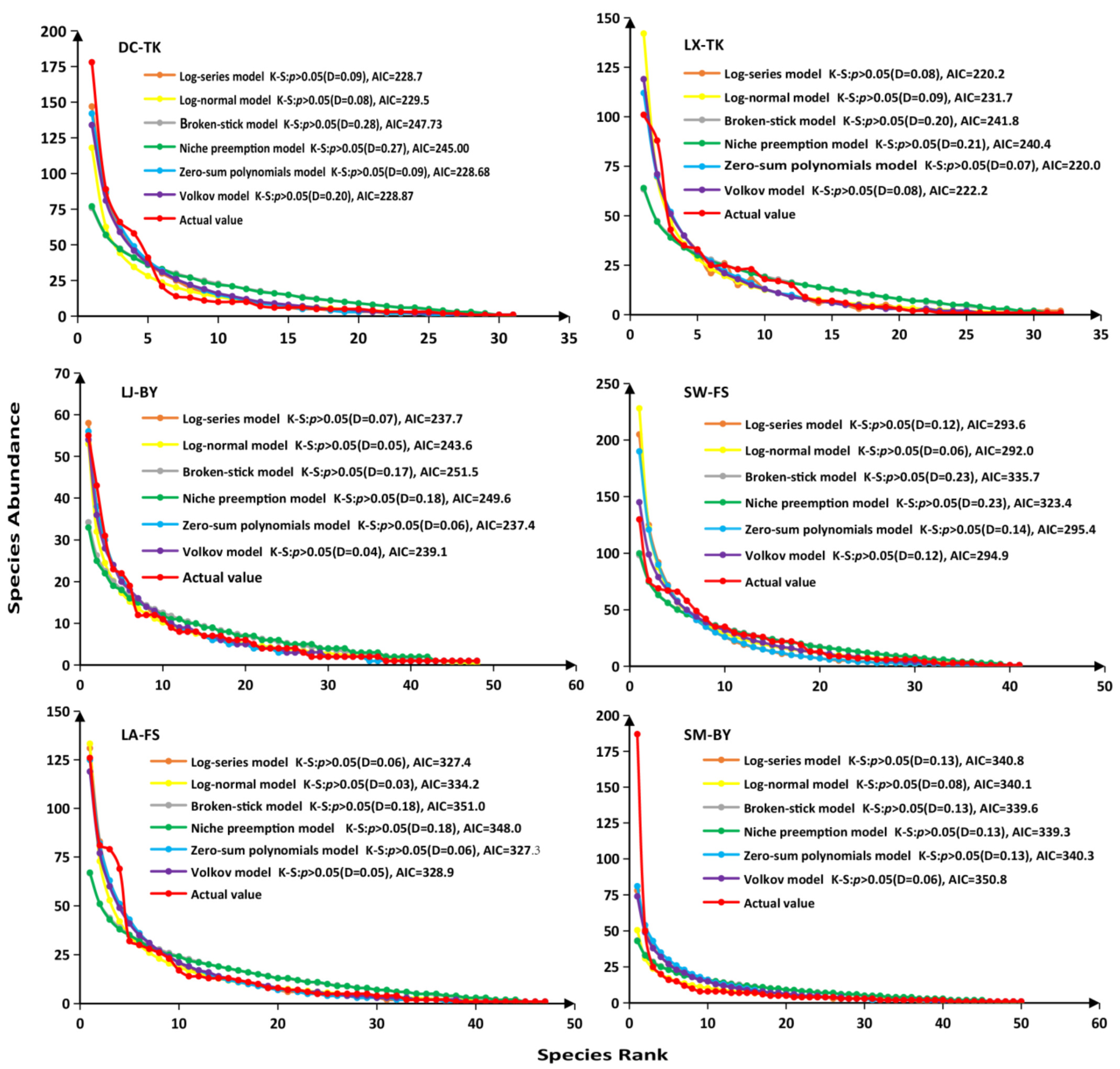
3.2. SADs Pattern in Tiankeng and Non-Tiankeng Forests

There was a significant difference in SADs patterns (Kruskal-Wallis chisq = 16.798, p < 0.05) between the Tiankeng and non-Tiankeng forests (Figure 2a). The species accumulation rate was highest in the fringe of Tiankeng forests and lowest in the inside of Tiankeng forests (Figure 2b). The Jaccard index showed that the species similarity between the fringe and inside of Tiankeng forests was the highest (0.36), followed by the non-Tiankeng forests, and the fringe of Tiankeng forests (0.29), and between the inside of Tiankeng forests and the non-Tiankeng forests was the lowest (0.27) (Figure 2c).

3.3. Goodness-of Fit of SADs Models in Tiankeng and Non-Tiankeng Forests

We observed differences in the test values at the 40m×40m scale between forests with different plots. K-S tests indicated that there were no significant differences between the simulated and actual SAD values and all models have passed the K-S test (p > 0.05) between Tiankeng and non-Tiankeng forests (Figure 3). The AIC test of goodness-of-fit results showed that the neutral models (△mean AIC = 1.3, AIC weights mean = 26.0%) performed better than the niche (△mean AIC = 22.7, AIC weights mean = 0.1%) and statistical models (△mean AIC = 2.7, AIC weights mean = 24.1%) in the Tiankeng forest, while the statistical models (△mean AIC = 2.4, AIC weights mean = 20.0%) performed better than the niche (△mean AIC = 11.2, AIC weights mean = 15.0%) and neutral (△mean AIC = 3.5, AIC weights mean = 15.1%) models in the non-Tiankeng forests. According to the results of neutral theory parameters and the species diversity (Table 2), the fundamental biodiversity number (θ), species immigration rate (m), species richness, and Shannon–Wiener index was the highest in the fringe of the Tiankeng forest and the lowest was in the inside the Tiankeng forests.

4. Discussion

4.1. Species Composition of Tiankeng Forest and Nearby Non-Tiankeng Forests

The species dispersal plays an important role in the structure, composition, and succession of vegetation [1]. The species dispersal from the inside of Tiankeng forests to the nearby non-Tiankeng forests is limited, while species have unlimited dispersal from nearby non-Tiankeng forests to the inside of Tiankeng forests via the fringe of Tiankeng forests. The unique negative topography of Tiankeng caused a huge surface drop that further influenced the species dispersal [26]. The natural geographical barrier caused by towering cliffs and the huge depth limited the species dispersal from the inside of Tiankeng forests to the nearby non-Tiankeng forests, hindering the evolution of species-specific communication. As a result, the species composition of Tiankeng forests was changed with vegetation landscape fragmentation. However, the internal enclosed environment of Tiankeng could be conducive to the independent evolution of species in the Tiankeng forests, which provided habitats for more precious and primitive species [24]. Instead, species have unlimited dispersal from nearby non-Tiankeng forests to the inside of Tiankeng forests. Some of the common species (Choerospondias axillaris B. L. Burtt & A. W. Hill and Rhaphiolepis indica Lindley) in the nearby non-Tiankeng forests were found in the Tiankeng forests to become dominant or rare species.
It is obvious that the phenomenon of single family, genera, and species were detected in study sites of Dashiwei Tiankeng Group. The results indicate that the population in the study area was a mosaic system formed by multiple local populations. Meanwhile, there are functional exchanges between the various populations in three habitats. Disturbance promoted the increase of species diversity, and community ecotones controlled the exchange of species between different ecosystems [43]. The fringe of the Tiankeng forest was an ecocritical place of species dispersal, while the nearby non-Tiankeng forest was a regional species pool for the inside of Tiankeng forests. Fragmented habitats in Dashiwei Tiankeng Group increase the probability of random extinction of vulnerable species in Tiankeng forests. However, the species dispersal between habitat patches can also rebuild a new population in those unoccupied spaces [44]. Therefore, we should protect the nearby non-Tiankeng forests for maintenance of the ecosystem in Tiankeng forests.

4.2. SADs Pattern in Tiankeng and Non-Tiankeng Forests

There were significant differences in the SAD pattern between the inner and outer fringe area of Tiankeng forest and nearby non-Tiankeng forest. Species accumulation in the fringe of Tiankeng forest was the largest, and most species in inner Tiankeng forests originated from nearby non-Tiankeng forests via the fringe area. On the one hand, the fringe of Tiankeng forest is surrounded by non-Tiankeng forest and encircles the inside of the Tiankeng forest [30]. The non-Tiankeng forest is usually distributed in the foothills, ridges, and slopes near villages and farmlands, and is greatly affected by human activities which enhance alien species to the Tiankeng forests [22,45]. On the other hand, the inside of the Tiankeng forest is located at the bottom of the negative topographic structure, and this benefits species accumulation.
The Tiankeng formation can be tracked back to the Paleocene [46]. At that time, species in this area would freely migrate. Later, the Tiankeng and the Tiankeng forests gradually evolved and formed along with the geological movement. By now, with global warming, nearby non-Tiankeng forests were suffering soil loss, water stress, and degradation, some species could not adapt to their stress environment and took refuge in the Tiankeng negative terrain [27,47]. Sufficient water and heat condition, stable growing environment, and tundra organic-rich soil in Tiankeng provide a favorable place for the heterogeneity and diversity of species [24,27]. Therefore, by comparing the SADs difference between Tiankeng and non-Tiankeng forests, we can determine that the Tiankeng forest is a plant refuge formed by surrounding species that have adapted to the environmental changes. One of the reasons is that the negative topographic structure promotes the accumulation of species, and the other is that the external environment deteriorates and species are attracted by the hot and humid environment of Tiankeng.

4.3. Goodness-of Fit of SADs Models in Tiankeng and Non-Tiankeng Forests

SAD is usually described by various fitting curves to reflect the influence of different ecological processes [1,6]. Our SAD results show that the neutral model has the smallest AIC value in Tiankeng forests, while the statistical model has the smallest AIC value in the non-Tiankeng forests. Therefore, in Tiankeng forests, the main driving force is the neutral process, and in non-Tiankeng forests, it is the niche and neutral processes. Why is there a difference? One reason may be related to community structure. In the early stages of growth, young trees are mainly affected by the neutral process and less affected by the niche process because they have weak biological characteristics and inter-specific competitiveness, and are vulnerable to the dangers of surface environment filtering and randomness [48]. As the species gradually grow, they not only enhance their biological characteristics, but also become increasingly affected by environmental filtering and the interaction between organisms. Finally, when species mature, the main community driving force is the niche process [31]. Tiankeng forest is an isolated natural secondary forest, the majority of plant individuals are in the growth period, and species relationship is mainly driven by heterogeneity of the habitat [27,30]. The negative topographic structure can protect the species from external interference, and strongly limits their dispersal from inside to outside in Tiankeng. Therefore, the neutral process plays an important role in the structure of the Tiankeng forest community, and this is one of the important points to incite Tiankeng forests being a plant refuge. However, the niche process is still evident with lesser influence [30]. Non-Tiankeng forests are near mountain secondary forests, of higher density, and with more younger trees than Tiankeng forests [22]. Additionally, their inter specific community relationships are more competitive and there is a fierce niche overlap and differentiation [22,30]. Thus, Tiankeng forests are more vulnerable to the neutral processes, while the non-Tiankeng forests are more readily affected by niche and neutral processes.
Another reason is lower human interference, and stronger erosion is a feature of negative terrain, compared to more unstable, vulnerable non-Tiankeng forest terrain [29]. The Dashiwei Tiankeng group is formed under the combined action of flowing water and gravity erosion [22]. The Tiankeng forest is situated in negative terrain and connected with the underground river, while the nearby non-Tiankeng forest is located in a downslope of karst rock mountain. This is the reason for which the Tiankeng forest suffered more hydraulic erosion and gravity erosion than non-Tiankeng. Therefore, as long as the topographical differences exist, the advantages in Tiankeng forests will continue. Additionally, this also raises conjecture, as the nearby non-Tiankeng forests were likely Tiankeng forests many years ago.
There are differences in aspects of species rarity, richness, migration rate, and accumulation rate between Tiankeng and nearby non-Tiankeng forests, but the ecological, niche, and neutral processes still work together in SADs. Some argued that niche and neutral processes are not mutually exclusive community forces, and that they are more like two endpoints in a continuous pattern, with a gradual transition phase between them [49]. In other words, any community may be able to find a corresponding position on the “niche-neutral continuum”. Therefore, there is a trade-off between the niche and the neutral processes in community; when influence of the niche process declines, it is accompanied by an increase in the role of the neutral process [50]. Additionally, the trade-off relationship between the niche and neutral processes is decided by the community structure, species characteristics, environmental changes, and the outside interference.
Both Tiankeng forests and non-Tiankeng forests are karst forests, but the former, as a small patch of karst forest in the southwest of China, is under the control of nearby non-Tiankeng forests through the Tiankeng forest fringe area. As an ecotone, the outer fringe area of Tiankeng forests is affected by the nearby non-Tiankeng forests [24] and then have an influence on the inner area of Tiankeng forest. For example, Manglietia aromatica Dandy, a representative refuge plant of Tiankeng forest, has only ever existed in Tiankeng forest and has never been found in nearby non-Tiankeng forests of the Dashiwei Tiankeng Group. Therefore, it appears that species have successfully migrated and established in the Tiankeng forest interior.
Fierce competition among species has always existed in the non-Tiankeng forest, and the degree of niche differentiation was high, but the Tiankeng forest on negative terrain has stable environmental conditions and is good at collecting soil, reserving water, and heat [30]. Therefore, some species that prefer wet and warm environments in non-Tiankeng forest will be attracted by the environmental conditions and continue to move to the negative terrain. Subsequently, with species migration and evolution, Tiankeng forest species will not only maintain their own characteristics, but also have similarities with nearby non-Tiankeng forest communities, illustrating that the local species composition is controlled by the regional community.
Different patterns of SAD may indicate specific environmental conditions. It is doubtful whether there would be other ecological processes that respond to the species co-occurrence. This is because each forests species has its own specific role as a result of evolutionary processes [41]. Moreover, multiple-mechanism models may have better results when fitting the same data. The model fitting results based solely on the patterns of species abundance cannot fully verify the ecological mechanism behind it. Therefore, we suggested that the neutral process was important for the SAD pattern in Tiankeng forests, a further analysis needs to be carried out in combination with environmental factors and spatial patterns.

5. Conclusions

The comparing of SADs between Tiankeng and non-Tiankeng forests is essential for its management, conservation, and sustainable utilization in Dashiwei Tiankeng Group. Assessing the role of biodiversity in Tiankeng forests could help in understanding climate change, approaches to the wise use of sustainable resources, preserving biological diversity, and exploring the community maintenance mechanism. For example, we found that the species dispersal from the inside of Tiankeng forests to the nearby non-Tiankeng forests is limited, while species has unlimited dispersal from nearby non-Tiankeng forests to the inside of Tiankeng forests via the fringe of Tiankeng forests. Moreover, some species in Tiankeng forest tend to become rarer and more precious. Therefore, this study’s results show that the neutral process incites Tiankeng forests to be a plant refuge throughout the fitting of niche and neutral models with nearby non-Tiankeng forests. Finally, the SAD pattern was related to the environment, climate, topography, and human activities. Tiankeng forests will remain its own unique ecosystem functions and ecological position if we enhance the protection of the nearby non-Tiankeng forest.

Author Contributions

L.H., H.Y., X.A., Y.Y., L.Y., G.H., X.L., M.C. and Y.X. conceived research idea, designed the research and collected field data. L.H., X.A. and L.Y. analyzed the data, L.H. and H.Y. wrote the first draft. L.H., H.Y., X.A., Y.Y., L.Y., G.H., X.L., M.C. and Y.X. All authors have read and agreed to the published version of the manuscript.

Funding

This work was supported by the National Natural Science Foundation of China (No. 31960047), the Guangxi Key Research and Development Program(No. AB21220057), the Research Funds of The Guangxi Key Laboratory of Landscape Resources Conservation and Sustainable Utilization in Lijiang River Basin, Guangxi Normal University (No. LRCSU21Z0101), and the Key Laboratory Research Foundation of Ecology of Rare and Endangered Species and Environmental Protection (Ministry of Education), Guangxi Normal University (No. ERESEP2019Z04).

Institutional Review Board Statement

Not applicable.

Informed Consent Statement

Not applicable.

Data Availability Statement

Data recorded in the current study are available in all Tables and Figures of the manuscript.

Acknowledgments

We are grateful to the workers at the Leye-Fengshan Global Geopark (China), who gave permission for, and contributed to, this research in Dashiwei Tiankeng Group. We also thank the locals of Shuaba village, Leye, China.

Conflicts of Interest

The authors declare that they have no known competing financial interest or personal relationships that could have influenced the work reported in this paper.

References

  1. Dong, K.; Hao, G.; Yang, N.; Zhang, J.; Ding, X.; Ren, H.; Shen, J.; Wang, J.; Jiang, L.; Zhao, N.; et al. Community assembly mechanisms and succession processes significantly differ among treatments during the restoration of Stipa grandis–Leymus chinensis communities. Sci. Rep. 2019, 9, 16289. [Google Scholar] [CrossRef] [PubMed]
  2. Schmitt, S.; Tysklind, N.; Derroire, G.; Heuertz, H.; Herault, B. Topography shapes the local coexistence of tree species within species complexes of Neotropical forests. Oecologia 2021, 196, 389–398. [Google Scholar] [CrossRef] [PubMed]
  3. Germain, R.M.; Mayfield, M.; Gilbert, B. The ‘filtering’ metaphor revisited: Competition and environment jointly structure invasibility and coexistence. Biol. Lett. 2018, 14, 20180460. [Google Scholar] [CrossRef] [PubMed] [Green Version]
  4. Magura, T.; Lövei, G.L.; Tóthmérész, B. Conversion from environmental filtering to randomness as assembly rule of ground beetle assemblages along an urbanization gradient. Sci. Rep. 2018, 8, 16992. [Google Scholar] [CrossRef] [PubMed] [Green Version]
  5. Yin, D.; Ye, D.; Cadotte, M.W. Habitat loss-biodiversity relationships are influenced by assembly processes and the spatial configuration of area loss. For. Ecol. Manag. 2021, 496, 119452. [Google Scholar] [CrossRef]
  6. Matthews, T.J.; Whittaker, R.J. Neutral theory and the species abundance distribution: Recent developments and prospects for unifying niche and neutral perspectives. Ecol. Evol. 2014, 4, 2263–2277. [Google Scholar] [CrossRef] [PubMed]
  7. Kusumoto, B.; Kubota, Y.; Baselga, A.; Gómez, C.; Odríguez, O.C.; Shiono, T. Community dissimilarity of angiosperm trees reveals deep-time diversification across tropical and temperate forests. J. Veg. Sci. 2021, 32, e13017. [Google Scholar] [CrossRef]
  8. Ma, K.M. Advances of the Study on Species Abundance Pattern. Chin. J. Plant Ecol. 2003, 3, 412–426. Available online: https://www.plant-ecology.com/CN/10.17521/cjpe.2003.0060 (accessed on 15 September 2021).
  9. Hidasi, N.J.; Bini, L.M.; Siqueira, T.; Cianciaruso, M.V. Ecological similarity explains species abundance distribution of small mammal communities. Acta Oecol. 2020, 102, 103502. [Google Scholar] [CrossRef]
  10. Waldock, C.; Stuart-Smith, R.D.; Albouy, C.; Cheung, W.; Edgar, G.J.; Mouillot, D.; Tjiputra, J.; Pellissier, L. A quantitative review of abundance-based species distribution models. Ecography 2022, 1, e05694. [Google Scholar] [CrossRef]
  11. Thierry, E.H. Stochastic species abundance models involving special copulas. Phys. A. 2018, 490, 77–91. [Google Scholar] [CrossRef]
  12. Latimer, A.; Wu, S.; Silander, G. Building statistical models to analyze species distributions. Ecol. Appl. 2006, 16, 33–50. [Google Scholar] [CrossRef] [PubMed] [Green Version]
  13. Takolander, A.; Hickler, T.; Meller, L.; Caneza, M. Comparing future shifts in tree species distributions across Europe projected by statistical and dynamic process-based models. Reg. Environ. Chang. 2019, 19, 251–266. [Google Scholar] [CrossRef] [Green Version]
  14. He, F.; Tang, D. Estimating the niche preemption parameter of the geometric series. Acta Oecologica 2008, 33, 105–107. [Google Scholar] [CrossRef]
  15. Dallas, T.; Hastings, A. Habitat suitability estimated by niche models is largely unrelated to species abundance. Glob. Ecol. Biogeogr. 2018, 27, 1448–1456. [Google Scholar] [CrossRef]
  16. Barabás, G.; Andrea, R.; Rael, R.; Meszéna, G.; Ostling, A. Emergent neutrality or hidden niches. Oikos 2013, 122, 1565–1572. [Google Scholar] [CrossRef] [Green Version]
  17. Petr, D.; Karolina, T.; Tereza, K. Linking species abundance and overyielding from experimental communities with niche and fitness characteristics. J. Ecol. 2019, 107, 178–189. [Google Scholar] [CrossRef]
  18. Volkov, I.; Banavar, J.R.; Hubbell, S.P.; Maritan, A. Neutral theory and relative species abundance in ecology. Nature 2003, 424, 1035–1037. [Google Scholar] [CrossRef] [PubMed] [Green Version]
  19. Wang, X.Z.; Ellwood, M.; Ai, D.; Zhang, R.Y.; Wang, G. Species abundance distributions as a proxy for the niche-neutrality continuum. J. Plant Ecol. 2018, 11, 445–452. [Google Scholar] [CrossRef]
  20. Villa, P.M.; Martins, S.V.; Rodrigues, A.C.; Alice, C.R.; Nathália, V.H.; Michael, A.C.; Ali, A. Testing species abundance distribution models in tropical forest successions: Implications for fine-scale passive restoration. J. Ecol. Eng. 2019, 135, 28–35. [Google Scholar] [CrossRef]
  21. Feng, G.; Huang, J.; Xu, Y.; Li, J.; Zhang, R. Disentangling environmental effects on the tree species abundance distribution and richness in a subtropical forest. Front. Plant Sci. 2021, 12, 367. [Google Scholar] [CrossRef] [PubMed]
  22. Zhu, X.W. Leye Tiankeng; Guangxi Science and Technology Publishing House: Nanning, China, 2018. (In Chinese) [Google Scholar]
  23. Lin, Y. Species Diversity of Karst Tiankeng Forest in Dashiwei Tiankengs, Guangxi. Master Thesis, College of life Sciences, Guangxi Normal University, Guilin, China, 2005. (In Chinese). [Google Scholar]
  24. Pu, G.; Lv, Y.; Dong, L.; Zhou, L.; Huang, K.; Zeng, D.; Mo, L.; Xu, G. Profiling the bacterial diversity in a typical Karst Tiankeng of China. Biomolecules 2019, 9, 187. [Google Scholar] [CrossRef] [Green Version]
  25. Zhu, S.F.; Jiang, C.; Shui, W.; Guo, P.P.; Zhang, Y.Y.; Feng, J. Vertical distribution characteristics of plant community in shady slope of degraded Tiankeng talus: A case study of Zhanyi Shenxiantang in Yunnan, China. J. Appl. Ecol. 2020, 31, 1496–1504. [Google Scholar] [CrossRef]
  26. Hong, S.K.; Song, I.J.; Wu, J. Fengshui theory in urban landscape planning. Urban Ecosyst. 2007, 10, 221–237. [Google Scholar] [CrossRef]
  27. Su, Y.Q.; Tang, Q.M.; Mo, F.Y.; Xue, Y.G. Karst Tiankengs as refugia for indigenous tree flora amidst a degraded landscape in southwestern China. Sci. Rep. 2017, 7, 4249. [Google Scholar] [CrossRef] [PubMed] [Green Version]
  28. Chen, J.; Lin, W.; Zhang, Y.; Dai, Y.; Chen, B. Village Fengshui Forests as Forms of Cultural and Ecological Heritage: Interpretations and Conservation Policy Implications from Southern China. Forests 2020, 11, 1286. [Google Scholar] [CrossRef]
  29. Wan, F.; Zhang, X.; Li, T. Stability analysis of Jiguanshan Tunnel construction under karst tiankeng. IOP Conf. Ser. EES 2021, 769, 32–54. Available online: https://schlr.cnki.net/Detail/doi/GARJ2021_1/SIPD0DEE5CEC6C628C2AF275723D00351265 (accessed on 8 December 2021). [CrossRef]
  30. Huang, L.J.; Yu, Y.M.; An, X.F.; Yu, L.L.; Xue, Y.G. Interspecific association of main woody plants in Tiankeng forests of Dashiwei Tiankeng Group, Guangxi. Guihaia 2021, 41, 695–706. (In Chinese) [Google Scholar] [CrossRef]
  31. Zhang, S.Z. Study on the Maintenance Mechanisms of Species Diversity in the Matural Old Growth Tropical Forests on the Hainan Island, China. Ph.D. Dissertation, Chinese Academy of Forestry, Beijing, China, 2017. (In Chinese). [Google Scholar]
  32. Wei, Y.; Wen, F.; Fu, L.; Xin, Z.; Jiang, R.; Pan, B.; Hua, F.; Mao, S.; Li, S.; Ma, H.; et al. The Distribution and Conservation Status of Native Plants in Guangxi, China; China Forestry Publishing: Beijing, China, 2018. [Google Scholar]
  33. Avolio, M.; Forrestel, E.J.; Chang, C.C.; La Pierre, K.J.; Burghardt, K.T.; Smith, M.D. Demystifying dominant species. New Phytol. 2019, 223, 1106–1126. [Google Scholar] [CrossRef] [PubMed]
  34. Skeen, J.N. An extension of the concept of importance value in analyzing forest communities. Ecology 1973, 54, 655–656. [Google Scholar] [CrossRef]
  35. Hadley, W.; Romain, F.; Lionel, H.; Kirill, M. Dplyr: A Grammar of Data Manipulation. R Package Version 1.0.0. 2020. Available online: https://CRAN.R-project.org/package=dplyr (accessed on 9 December 2021).
  36. R Core Team. R: A Language and Environment for Statistical Computing; R Foundation for Statistical Computing: Vienna, Austria, 2020; Available online: https://www.R-project.org/ (accessed on 8 December 2021).
  37. Keylock, C.J. Simpson diversity and the Shannon-wiener index as special cases of a generalized entropy. Oikos 2005, 109, 203–207. [Google Scholar] [CrossRef]
  38. Fletcher, S.; Islam, M. Comparing sets of patterns with the Jaccard index. Asian-Australas. J. Anim. Sci. 2018, 22, 1–17. [Google Scholar] [CrossRef] [Green Version]
  39. Fisher, C.K.; Mehta, P. The transition between the niche and neutral regimes in ecology. Proc. Natl. Acad. Sci. USA 2014, 111, 13111–13116. [Google Scholar] [CrossRef] [PubMed] [Green Version]
  40. Alonso, D.; Mckane, A.J. Sampling Hubbell’s neutral theory of biodiversity. Ecol. Lett. 2004, 7, 901–910. [Google Scholar] [CrossRef]
  41. Ramesh, T. Trends and Changes in Hydroclimatic Variable; Elsevier: Cambridge, MA, USA, 2018. [Google Scholar]
  42. Paulo, I.P.; Murilo, D.M.; Andre, C. Maximum Likelihood Models for Species Abundance Distributions. R Packages Version 0.4.2. 2018. Available online: http://piLaboratory.github.io/sads (accessed on 8 December 2021).
  43. Muluneh, M.; Feyissa, M.; Wolde, T. Effect of forest fragmentation and disturbance on diversity and structure of woody species in dry Afromontane forests of northern Ethiopia. Biodivers. Conserv. 2021, 30, 1753–1779. [Google Scholar] [CrossRef]
  44. Bertassello, L.; Bertuzzo, E.; Botter, G.; Jawitz, J.W.; Aubeneau, A.F.; Hoverman, J.T.; Rinaldo, A.; Rao, P.S.C. Dynamic spatio-temporal patterns of metapopulation occupancy in patchy habitats. R. Soc. Open. Sci. 2021, 8, 201309. [Google Scholar] [CrossRef] [PubMed]
  45. Chen, B.X.; Coggins, C.; Minor, J.; Zhang, Y.Q. Fengshui forests and village landscapes in China: Geographic extent, socioecological significance, and conservation prospects. Urban For. Urban Green. 2018, 31, 79–92. [Google Scholar] [CrossRef]
  46. Shen, H.T.; Kimikazu, S.; Qi, M.; Masumi, M.; Tetsuya, M.; Seiji, H.; Takahashi, T.; Honda, M.; Sueki, K.; He, M.; et al. Exposure age dating of Chinese Tiankengs by 36Cl-AMS. Nucl. Instrum. Methods B 2019, 459, 29–35. [Google Scholar] [CrossRef]
  47. Yang, G.; Peng, C.; Liu, Y.; Dong, F.Q. Tiankeng: An ideal place for climate warming research on forest ecosystems. Environ. Earth Sci. 2019, 78, 46. [Google Scholar] [CrossRef]
  48. Wang, Y.; Lamontagne, J.M.; Lin, F.; Yuan, Z.Q.; Ye, J.; Wang, X.G.; Hao, Z. Similarity between seed rain and neighbouring mature tree communities in an old-growth temperate forest. J. For. Res. 2019, 31, 2435–2444. [Google Scholar] [CrossRef] [Green Version]
  49. Niccolo, A.; Jorge, H.; Carlos, A.P.; Tommaso, B.; Amos, M.; Samir, S. Neutral and niche forces as drivers of species selection. J. Theor. Biol. 2019, 483, 109969. [Google Scholar] [CrossRef]
  50. Pinsky, M.L. Species coexistence through competition and rapid evolution. Proc. Natl. Acad. Sci. USA 2019, 116, 2407–2409. [Google Scholar] [CrossRef] [PubMed] [Green Version]
Figure 1. Map of the study area including the plot location. Sample sites in Dashiwei Tiankeng Group, Leye, China (a,b). Location of three habitats (ce), the nearby non-Tiankeng forest (c), the fringe of Tiankeng forest (d), and the inside of Tiankeng forest (e). Maps are created with ArcMap 10.5. Data map source from the Ministry of natural resources, PRC (http://www.mnr.gov.cn/, figure number: GS(2016)1595, accessed on 23 November 2021), Geospatial data cloud, Chinese Academy of Sciences (http://www.gscloud.cn/, accessed on 23 November 2021).
Diversity 14 00064 g001
Figure 2. ECDF curve (a), species-abundance curve (b), and Jaccard similarity index (c) at different sites of Dashiwei Tiankeng Group.
Diversity 14 00064 g002
Figure 3. The SADs and models fitting for woody plants at the 40 m × 40 m scale in Tiankeng and non-Tiankeng forests. The actual values are the observed abundance.
Diversity 14 00064 g003
Table 1. The importance value of dominant species at different sites of Dashiwei Tiankeng Group.
SpeciesThe Inside of Tiankeng ForestsThe Fringe of Tiankeng ForestsNearby Non-Tiankeng Forests
DC-TKLX-TKLJ-BYSM-BYLA-FSSW-FS
Lindera glauca (Sieb. et Zucc.) Bl.29.82%9.27%----
Schefflera guizhouensis C. B. Shang21.44%4.85%----
Miliusa sinensis Finet et Gagnep.11.29%-----
Machilus chinensis (Champ. ex Benth.) Hemsl.10.69%-3.88%---
Handeliodendron bodinieri (Lévl.) Rehd.4.90%12.32%6.05%2.18%2.91%3.38%
Choerospondias axillaris (Roxb.) B. L. Burtt & A. W. Hill5.72%10.97%19.61%-3.81%4.84%
Lindera pulcherrima var. Hemsleyana (Diels) H.P.Tsui1.29%9.90%5.78%-2.97%1.10%
Ilex macrocarpa Oliv.--10.83%-4.79%9.99%
Itea macrophylla Wall. ex Roxb.--10.05%---
Machilus glaucifolia S. K. Lee & F. N. Wei--8.97%15.39%--
Celtis sinensis Pers.1.10%8.61%2.67%-11.70%7.84%
Rhaphiolepis indica (Linnaeus) Lindley-1.73%1.64%-3.15%12.54%
Illicium simonsii Maxim.----10.82%-
Cinnamomum bodinieri Lévl.--2.47%-1.05%10.45%
Litsea rotundifolia var. Oblongifolia (Nees) Allen-1.62%9.78%-1.26%-
Itea yunnanensis Franch.-8.20%8.82%-5.83%9.61%
Table 2. Neutral theory parameter and species diversity.
Neutral Theory ParameterSpecies Diversity Index
Volkov ModelZero-Sum Polynomials Model
SitesθmθSpecies richnessShannon-Wiener index
DC-TK8.310.356.71313.81
LX-TK7.30.47.24323.64
LJ-BY16.650.5914.28484.63
SM-BY15.340.6212.44504.40
LA-FS13.340.4111.12474.33
SW-FS14.750.4211.86414.25
Publisher’s Note: MDPI stays neutral with regard to jurisdictional claims in published maps and institutional affiliations.

