Plant Diversity Patterns and Conservation Implications under Climate-Change Scenarios in the Mediterranean: The Case of Crete (Aegean, Greece)

 , , , ,
Abstract
:
1. Introduction
2. Materials and Methods
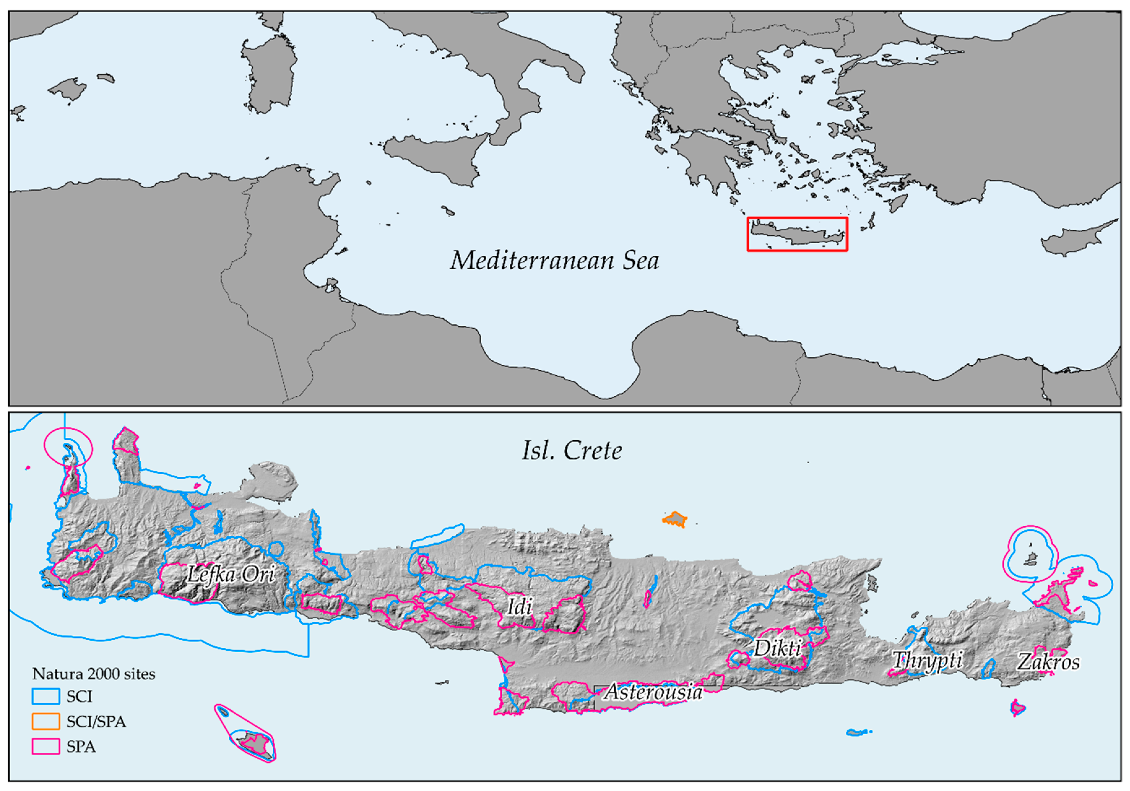
2.1. Study Area
2.2. Environmental Data
2.3. Climatic Refugia
2.4. Species Occurrence Data
2.5. Phylogenetic Tree
2.6. Species Distribution Models
2.6.1. Model Parameterisation and Evaluation
2.6.2. Model Projections
2.6.3. Area Range Change
2.6.4. Hotspots
2.7. IUCN Measures
2.8. Niche Breadth
2.9. GDM Analysis
2.10. Current and Future Spatial EDGE Patterns
2.11. Protected Area Network and Climatic Refugia Overlap
3. Results
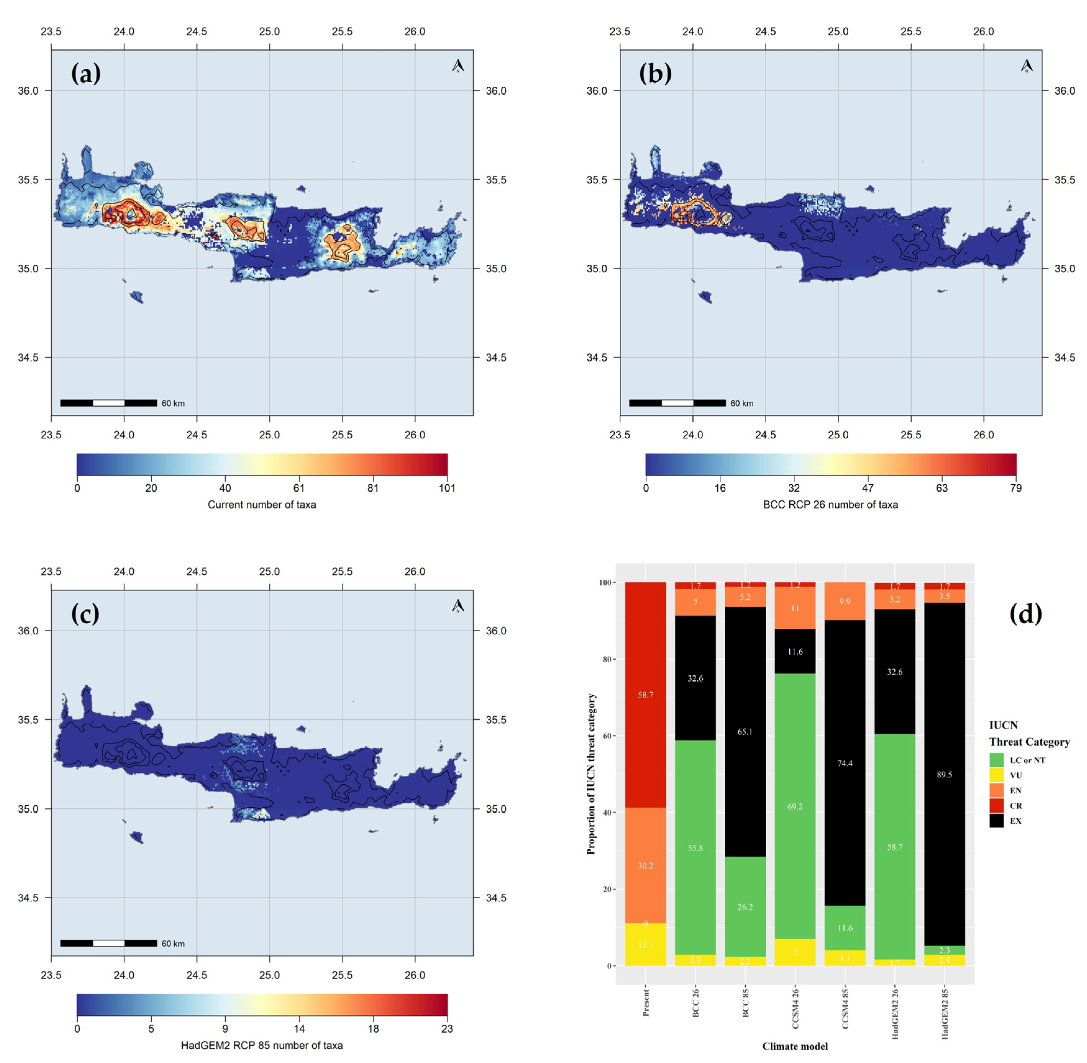
3.1. Species Distribution Models
3.1.1. Model Performance
3.1.2. Area Range Change
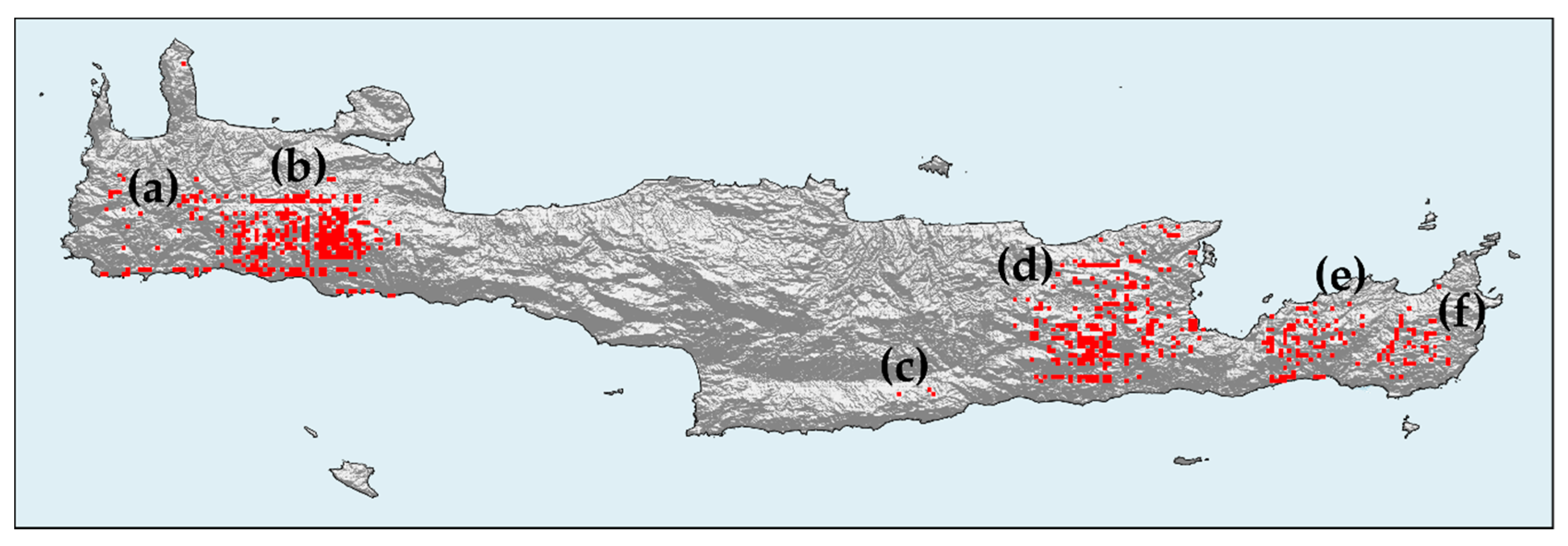
3.1.3. Hotspot Analysis
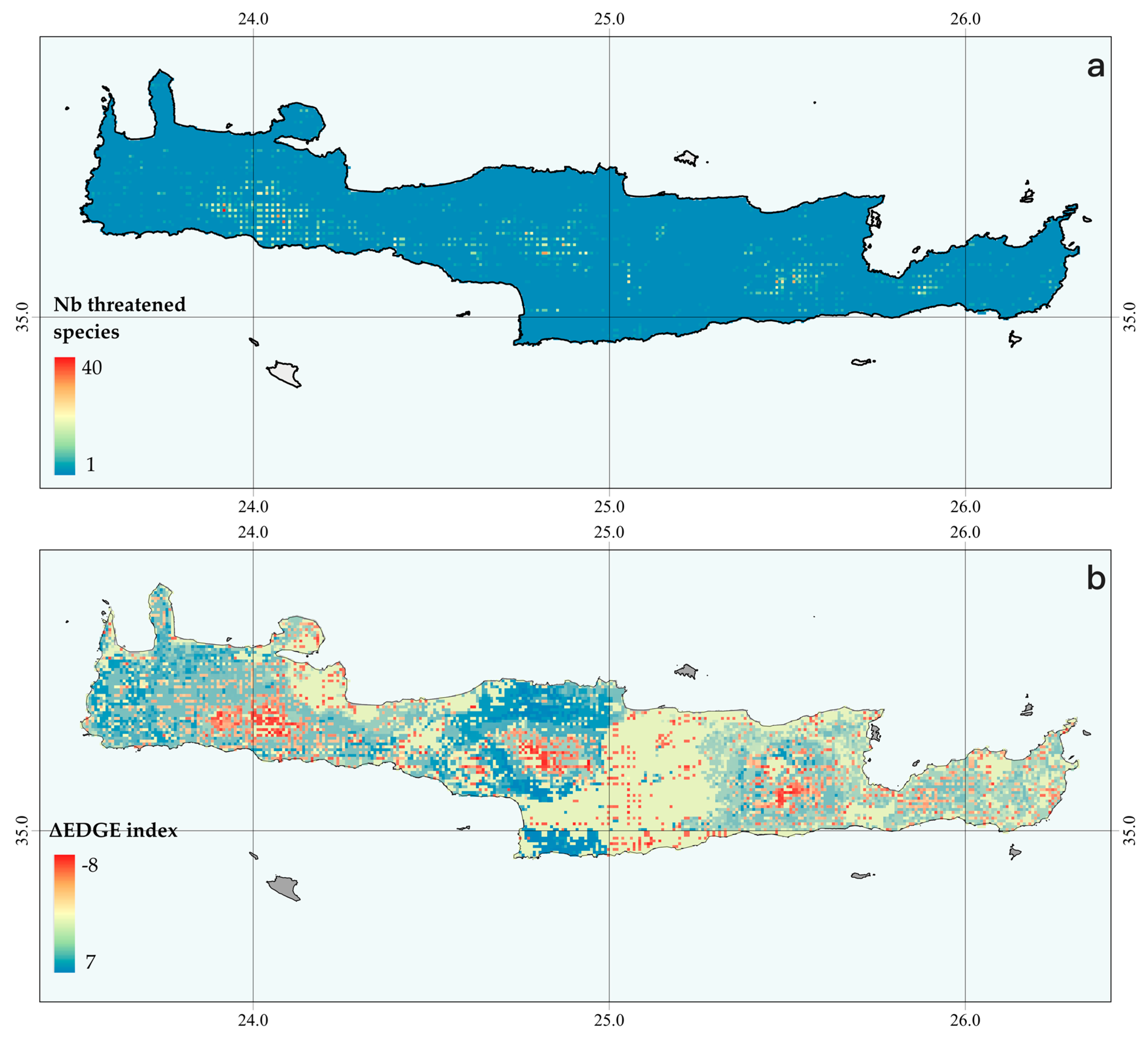
3.2. IUCN Measures
3.3. Niche Breadth
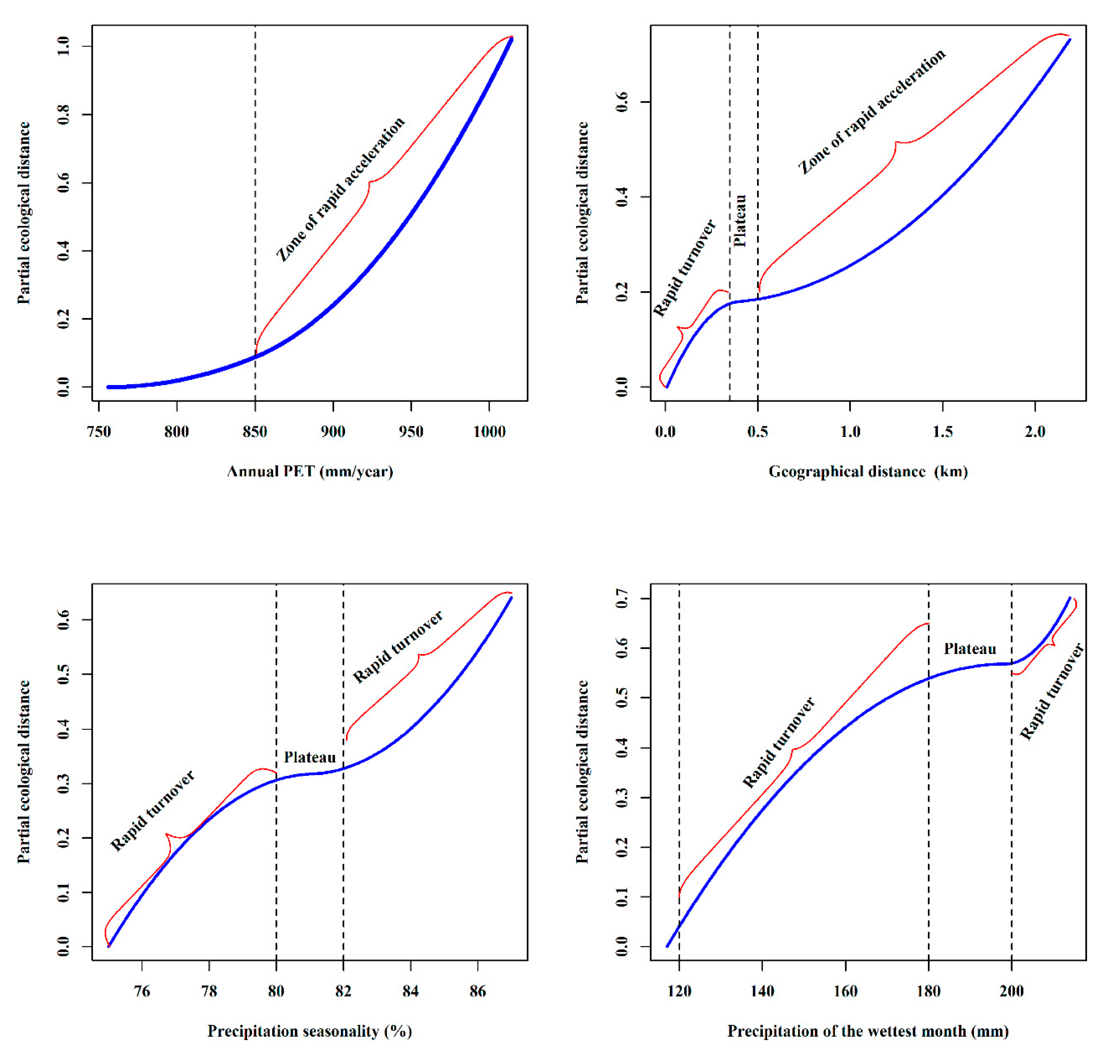
3.4. GDM Analysis
3.5. EDGE-Phylogenetic Diversity
3.6. Current and Future Spatial EDGE Patterns
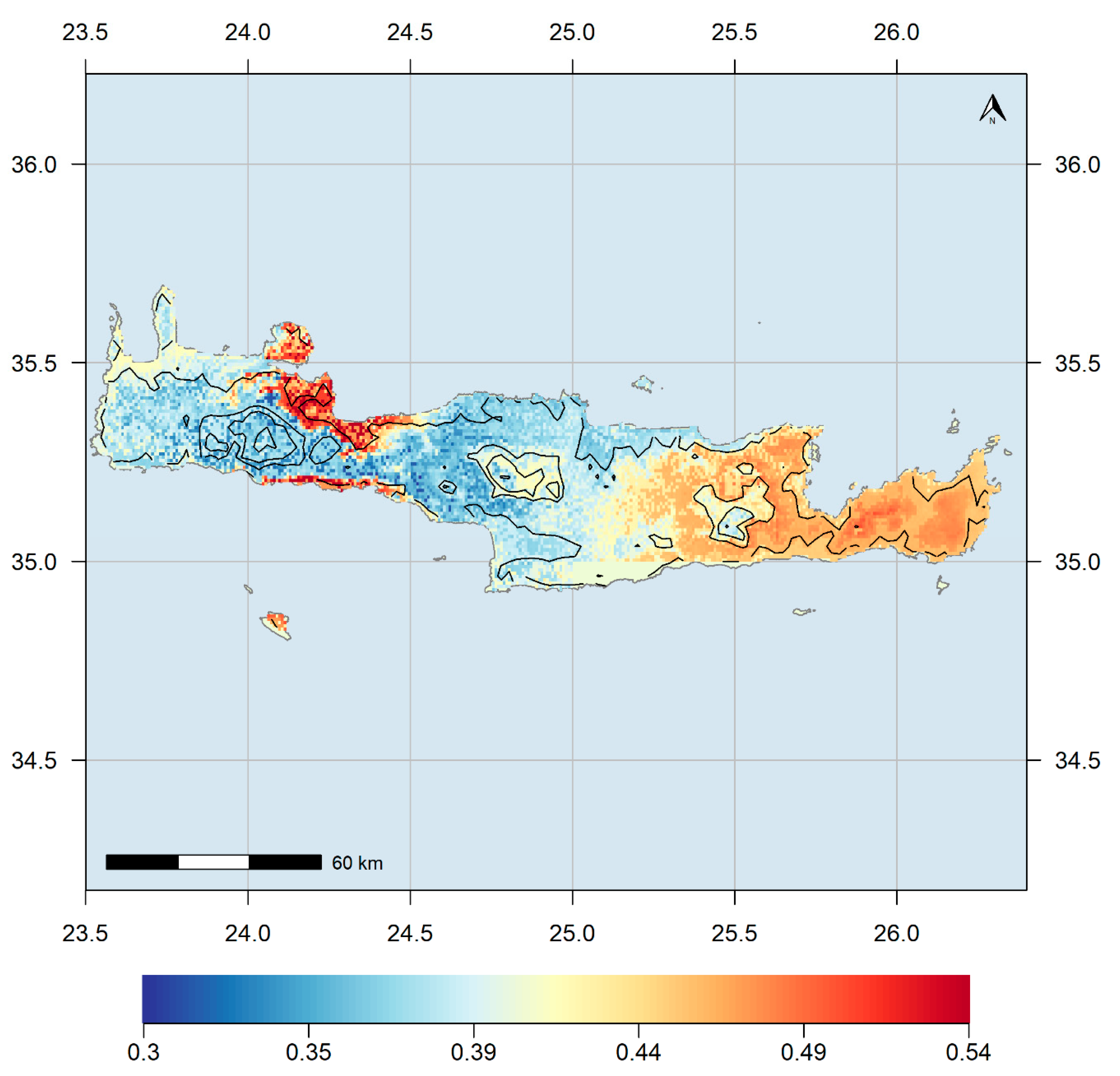
3.7. Climatic Refugia and Protected Area Network Overlap
4. Discussion
4.1. Diversity Hotspots
4.2. Conservation Assessment
4.3. Conservation and Management Implications
5. Conclusions
Supplementary Materials
Author Contributions
Funding
Conflicts of Interest
References
- Zalasiewicz, J.; Waters, C.N.; Williams, M.; Barnosky, A.D.; Cearreta, A.; Crutzen, P.; Ellis, E.; Ellis, M.A.; Fairchild, I.J.; Grinevald, J.; et al. When did the Anthropocene begin? A mid-twentieth century boundary level is stratigraphically optimal. Quat. Int. 2015, 383, 196–203. [Google Scholar] [CrossRef] [Green Version]
- Urban, M.C.; Bocedi, G.; Hendry, A.P.; Mihoub, J.B.; Peer, G.; Singer, A.; Bridle, J.R.; Crozier, L.G.; De Meester, L.; Godsoe, W.; et al. Improving the forecast for biodiversity under climate change. Science 2016, 353, aad8466. [Google Scholar] [CrossRef] [PubMed] [Green Version]
- Warren, R.; Vanderwal, J.; Price, J.; Welbergen, J.A.; Atkinson, I.; Ramirez-Villegas, J.; Osborn, T.J.; Jarvis, A.; Shoo, L.P.; Williams, S.E.; et al. Quantifying the benefit of early climate change mitigation in avoiding biodiversity loss. Nat. Clim. Chang. 2013, 3, 678–682. [Google Scholar] [CrossRef] [Green Version]
- Newbold, T. Future effects of climate and land-use change on terrestrial vertebrate community diversity under different scenarios. Proc. R. Soc. B Biol. Sci. 2018, 285, 20180792. [Google Scholar] [CrossRef] [PubMed]
- Halley, J.M.; Monokrousos, N.; Mazaris, A.D.; Vokou, D. Extinction debt in plant communities: Where are we now? J. Veg. Sci. 2017, 28, 459–461. [Google Scholar] [CrossRef] [Green Version]
- Wing, S.L. Mass Extinctions in Plant Evolution; Cambridge University Press: Cambridge, UK, 2004. [Google Scholar]
- Urban, M.C. Accelerating extinction risk from climate change. Science 2015, 348, 571–573. [Google Scholar] [CrossRef] [Green Version]
- Fischlin, A.; Midgley, G.; Price, J.; Leemans, R.; Gopal, B.; Turley, C.; Rounsevell, M.; Dube, P.; Tarazona, J.; Velichko, A. Ecosystems Their Properties Goods and Services. Climate Change 2007: Impacts Adaptation and Vulnerability. Contribution of Working Group II to the Fourth Assessment Report of the Intergovernmental Panel on Climate Change; Parry, M.L., Canziani, O.F., Palu, J.P., Eds.; Cambridge University Press: Cambridge, UK, 2007. [Google Scholar]
- IPCC Summary for Policymakers. Global Warming of 1.5 °C. An IPCC Special Report on the Impacts of Global Warming of 1.5 °C above Pre-Industrial Levels and Related Global Greenhouse gas Emission Pathways, in the Context of Strengthening the Global Response to the Threat of Climate Change; World Meteorological Organization: Geneva, Switzerland, 2018; ISBN 9789291691517. [Google Scholar]
- Groves, C.R.; Game, E.T.; Anderson, M.G.; Cross, M.; Enquist, C.; Ferdaña, Z.; Girvetz, E.; Gondor, A.; Hall, K.R.; Higgins, J.; et al. Incorporating climate change into systematic conservation planning. Biodivers. Conserv. 2012, 21, 1651–1671. [Google Scholar] [CrossRef]
- Sandel, B.; Arge, L.; Dalsgaard, B.; Davies, R.G.; Gaston, K.J.; Sutherland, W.J.; Svenning, J.C. The influence of late quaternary climate-change velocity on species endemism. Science 2011, 334, 660–664. [Google Scholar] [CrossRef] [Green Version]
- Médail, F. The specific vulnerability of plant biodiversity and vegetation on Mediterranean islands in the face of global change. Reg. Environ. Chang. 2017, 17, 1775–1790. [Google Scholar] [CrossRef] [Green Version]
- Médail, F.; Myers, N. Mediterranean Basin; Mittermeier, C.G., Lamoreux, J., Fonseca, G.A.B., Eds.; Sierra: Cheyenne, WY, USA, 2004. [Google Scholar]
- Médail, F.; Diadema, K. Glacial refugia influence plant diversity patterns in the Mediterranean Basin. J. Biogeogr. 2009, 36, 1333–1345. [Google Scholar] [CrossRef]
- Thackeray, S.J.; Henrys, P.A.; Hemming, D.; Bell, J.R.; Botham, M.S.; Burthe, S.; Helaouet, P.; Johns, D.G.; Jones, I.D.; Leech, D.I.; et al. Phenological sensitivity to climate across taxa and trophic levels. Nature 2016, 535, 241–245. [Google Scholar] [CrossRef] [PubMed] [Green Version]
- Urban, M.C. Escalator to extinction. Proc. Natl. Acad. Sci. USA 2018, 115, 11871–11873. [Google Scholar] [CrossRef] [PubMed] [Green Version]
- Pacifici, M.; Foden, W.B.; Visconti, P.; Watson, J.E.M.; Butchart, S.H.M.; Kovacs, K.M.; Scheffers, B.R.; Hole, D.G.; Martin, T.G.; Akçakaya, H.R.; et al. Assessing species vulnerability to climate change. Nat. Clim. Chang. 2015, 5, 215–224. [Google Scholar] [CrossRef]
- Giorgi, F.; Lionello, P. Climate change projections for the Mediterranean region. Glob. Planet. Chang. 2008, 63, 90–104. [Google Scholar] [CrossRef]
- Domina, G.; Bazan, G.; Campisi, P.; Greuter, W. Taxonomy and conservation in Higher Plants and Bryophytes in the Mediterranean Area. Biodivers. J. 2015, 6, 197–204. [Google Scholar]
- Phitos, D.; Constantinidis, T.H.; Kamari, G. The Red Data Book of Rare and Threatened Plants of Greece; Vololum II (EZ); Hellenic Botanical Society: Patra, Greece, 2009. [Google Scholar]
- Morelli, F.; Møller, A.P. Pattern of evolutionarily distinct species among four classes of animals and their conservation status: A comparison using evolutionary distinctiveness scores. Biodivers. Conserv. 2018, 27, 381–394. [Google Scholar] [CrossRef]
- Cadotte, M.W.; Cardinale, B.J.; Oakley, T.H. Evolutionary history and the effect of biodiversity on plant productivity. Proc. Natl. Acad. Sci. USA 2008, 105, 17012–17017. [Google Scholar] [CrossRef] [Green Version]
- Veron, S.; Faith, D.P.; Pellens, R.; Pavoine, S. Priority areas for phylogenetic diversity: Maximising gains in the mediterranean basin. In Phylogenetic Diversity: Applications and Challenges in Biodiversity Science; Springer International Publishing: Cham, Switzerland, 2018; pp. 145–166. ISBN 9783319931449. [Google Scholar]
- Foden, W.B.; Young, B.E.; Akçakaya, H.R.; Garcia, R.A.; Hoffmann, A.A.; Stein, B.A.; Thomas, C.D.; Wheatley, C.J.; Bickford, D.; Carr, J.A.; et al. Climate change vulnerability assessment of species. Wiley Interdiscip. Rev. Clim. Chang. 2019, 10, e551. [Google Scholar] [CrossRef] [Green Version]
- Berry, P.M.; Betts, R.A.; Harrison, P.A.; Sanchez-Arcilla, A. High-End Climate Change in Europe; Pensoft Publishers: Sofia, Bulgaria, 2017. [Google Scholar]
- Higgins, M.D. Greek islands, geology. In Encyclopedia of Islands; University of California Press: California, CA, USA, 2009; pp. 392–396. [Google Scholar]
- Sakellariou, D.; Galanidou, N. Pleistocene submerged landscapes and Palaeolithic archaeology in the tectonically active Aegean region. Geol. Soc. Lond. Spec. Publ. 2016, 411, 145–178. [Google Scholar] [CrossRef]
- Manzi, V.; Gennari, R.; Hilgen, F.; Krijgsman, W.; Lugli, S.; Roveri, M.; Sierro, F.J. Age refinement of the Messinian salinity crisis onset in the Mediterranean. Terra Nova 2013, 25, 315–322. [Google Scholar] [CrossRef]
- Hijmans, R.J.; Cameron, S.E.; Parra, J.L.; Jones, P.G.; Jarvis, A. Very high resolution interpolated climate surfaces for global land areas. Int. J. Climatol. 2005, 25, 1965–1978. [Google Scholar] [CrossRef]
- Title, P.O.; Bemmels, J.B. ENVIREM: An expanded set of bioclimatic and topographic variables increases flexibility and improves performance of ecological niche modeling. Ecography (Cop.) 2018, 41, 291–307. [Google Scholar] [CrossRef] [Green Version]
- McSweeney, C.F.; Jones, R.G.; Lee, R.W.; Rowell, D.P. Selecting CMIP5 GCMs for downscaling over multiple regions. Clim. Dyn. 2015, 44, 3237–3260. [Google Scholar] [CrossRef] [Green Version]
- Hengl, T.; de Jesus, J.M.; Heuvelink, G.B.M.; Gonzalez, M.R.; Kilibarda, M.; Blagotić, A.; Shangguan, W.; Wright, M.N.; Geng, X.; Bauer-Marschallinger, B.; et al. SoilGrids250m: Global gridded soil information based on machine learning. PLoS ONE 2017, 12, e0169748. [Google Scholar] [CrossRef] [PubMed] [Green Version]
- Jarvis, A.; Reuter, H.I.; Nelson, A.; Guevara, E. Hole-filled SRTM for the Globe Version 4. CGIAR-CSI SRTM 90 m Database. 2008. Available online: http//srtm.csi.cgiar.Org (accessed on 14 October 2019).
- Hijmans, R.J. raster: Geographic Data Analysis and Modeling 2018. Available online: https://CRAN.R-project.org/package=raster (accessed on 14 October 2019).
- Dormann, C.F.; Elith, J.; Bacher, S.; Buchmann, C.; Carl, G.; Carré, G.; Marquéz, J.R.G.; Gruber, B.; Lafourcade, B.; Leitão, P.J.; et al. Collinearity: A review of methods to deal with it and a simulation study evaluating their performance. Ecography (Cop.) 2013, 36, 27–46. [Google Scholar] [CrossRef]
- Naimi, B.; Hamm, N.A.S.; Groen, T.A.; Skidmore, A.K.; Toxopeus, A.G. Where is positional uncertainty a problem for species distribution modelling? Ecography (Cop.) 2014, 37, 191–203. [Google Scholar] [CrossRef]
- Owens, H.L.; Guralnick, R. climateStability: An R package to estimate climate stability from time-slice climatologies. Biodivers. Inform. 2019, 14, 8–13. [Google Scholar] [CrossRef] [Green Version]
- Brown, J.L.; Hill, D.J.; Dolan, A.M.; Carnaval, A.C.; Haywood, A.M. Paleoclim, high spatial resolution paleoclimate surfaces for global land areas. Sci. Data 2018, 5, 1–9. [Google Scholar] [CrossRef] [Green Version]
- Gamisch, A. Oscillayers: A dataset for the study of climatic oscillations over Plio-Pleistocene time-scales at high spatial-temporal resolution. Glob. Ecol. Biogeogr. 2019, 28, 1552–1560. [Google Scholar] [CrossRef] [Green Version]
- Owens, H. climateStability: Estimating Climate Stability from Climate Model Data. R Package, Version 0.1.1. Available online: https://CRAN.R-project.org/package=climateStability (accessed on 14 October 2019).
- Ashcroft, M.B. Identifying refugia from climate change. J. Biogeogr. 2010, 37, 1407–1413. [Google Scholar] [CrossRef]
- Dimopoulos, P.; Raus, T.; Bergmeier, E.; Constantinidis, T.; Iatrou, G.; Kokkini, S.; Strid, A.; Tzanoudakis, D. Vascular Plants of Greece: An Annotated Checklist; Botanic Garden and Botanical Museum Berlin-Dahlem: Berlin, Germany, 2013. [Google Scholar]
- Dimopoulos, P.; Raus, T.; Bergmeier, E.; Constantinidis, T.; Iatrou, G.; Kokkini, S.; Strid, A.; Tzanoudakis, D. Willdenowia—Ann Botanical Garden and Botanical Museum Berlin-Dahlem; Botanic Garden and Botanical Museum Berlin-Freie Universität Berlin: Berlin, Germany, 2016; Volume 46, pp. 301–347. [Google Scholar]
- Strid, A. Atlas of the Aegean Flora; Botanic Garden and Botanical Museum Berlin-Freie Universität Berlin: Berlin, Germany, 2016. [Google Scholar]
- van Proosdij, A.S.J.; Sosef, M.S.M.; Wieringa, J.J.; Raes, N. Minimum required number of specimen records to develop accurate species distribution models. Ecography 2016, 39, 542–552. [Google Scholar] [CrossRef]
- Elith, J.; Kearney, M.; Phillips, S. The art of modelling range-shifting species. Methods Ecol. Evol. 2010, 1, 330–342. [Google Scholar] [CrossRef]
- Aiello-Lammens, M.E.; Boria, R.A.; Radosavljevic, A.; Vilela, B.; Anderson, R.P. spThin: An R package for spatial thinning of species occurrence records for use in ecological niche models. Ecography (Cop.) 2015, 38, 541–545. [Google Scholar] [CrossRef]
- Robertson, M.P.; Visser, V.; Hui, C. Biogeo: An R package for assessing and improving data quality of occurrence record datasets. Ecography (Cop.) 2016, 39, 394–401. [Google Scholar] [CrossRef] [Green Version]
- Zizka, A.; Antonelli, A.; Silvestro, D. Sampbias, a Method for Quantifying Geographic Sampling Biases in Species Distribution Data. BioRxiv 2020. [Google Scholar] [CrossRef] [Green Version]
- Smith, S.A.; Brown, J.W. Constructing a broadly inclusive seed plant phylogeny. Am. J. Bot. 2018, 105, 302–314. [Google Scholar] [CrossRef] [Green Version]
- Jin, Y.; Qian, H.V. PhyloMaker: An R package that can generate very large phylogenies for vascular plants. Ecography (Cop.) 2019, 42, 1353–1359. [Google Scholar] [CrossRef] [Green Version]
- Bruelheide, H.; Dengler, J.; Jiménez-Alfaro, B.; Purschke, O.; Hennekens, S.M.; Chytrý, M.; Pillar, V.D.; Jansen, F.; Kattge, J.; Sandel, B.; et al. sPlot–A new tool for global vegetation analyses. J. Veg. Sci. 2019, 30, 161–186. [Google Scholar] [CrossRef]
- Maitner, B.S.; Boyle, B.; Casler, N.; Condit, R.; Donoghue, J.; Durán, S.M.; Guaderrama, D.; Hinchliff, C.E.; Jørgensen, P.M.; Kraft, N.J.B.; et al. The bien r package: A tool to access the Botanical Information and Ecology Network (BIEN) database. Methods Ecol. Evol. 2018, 9, 373–379. [Google Scholar] [CrossRef] [Green Version]
- Davies, T.J.; Kraft, N.J.B.; Salamin, N.; Wolkovich, E.M. Incompletely resolved phylogenetic trees inflate estimates of phylogenetic conservatism. Ecology 2012, 93, 242–247. [Google Scholar] [CrossRef] [Green Version]
- Kembel, S.W.; Cowan, P.D.; Helmus, M.R.; Cornwell, W.K.; Morlon, H.; Ackerly, D.D.; Blomberg, S.P.; Webb, C.O. Picante: R tools for integrating phylogenies and ecology. Bioinformatics 2010, 26, 1463–1464. [Google Scholar] [CrossRef] [Green Version]
- Isaac, N.J.B.; Turvey, S.T.; Collen, B.; Waterman, C.; Baillie, J.E.M. Mammals on the EDGE: Conservation Priorities Based on Threat and Phylogeny. PLoS ONE 2007, 2, e296. [Google Scholar] [CrossRef] [Green Version]
- Faith, D.P. Conservation evaluation and phylogenetic diversity. Biol. Conserv. 1992, 61, 1–10. [Google Scholar] [CrossRef]
- Tsirogiannis, C.; Sandel, B. PhyloMeasures: A package for computing phylogenetic biodiversity measures and their statistical moments. Ecography (Cop.) 2016, 39, 709–714. [Google Scholar] [CrossRef]
- Mazel, F.; Renaud, J.; Guilhaumon, F.; Mouillot, D.; Gravel, D.; Thuiller, W. Mammalian phylogenetic diversity-area relationships at a continental scale. Ecology 2015, 96, 2814–2822. [Google Scholar] [CrossRef] [Green Version]
- Thuiller, W.; Lafourcade, B.; Engler, R.; Araújo, M.B. BIOMOD-A platform for ensemble forecasting of species distributions. Ecography (Cop.) 2009, 32, 369–373. [Google Scholar] [CrossRef]
- Araújo, M.B.; New, M. Ensemble forecasting of species distributions. Trends Ecol. Evol. 2007, 22, 42–47. [Google Scholar] [CrossRef] [PubMed]
- Araújo, M.B.; Anderson, R.P.; Barbosa, A.M.; Beale, C.M.; Dormann, C.F.; Early, R.; Garcia, R.A.; Guisan, A.; Maiorano, L.; Naimi, B.; et al. Standards for distribution models in biodiversity assessments. Sci. Adv. 2019, 5, eaat4858. [Google Scholar] [CrossRef] [PubMed] [Green Version]
- Barbet-Massin, M.; Jiguet, F.; Albert, C.H.; Thuiller, W. Selecting pseudo-absences for species distribution models: How, where and how many? Methods Ecol. Evol. 2012, 3, 327–338. [Google Scholar] [CrossRef]
- Valavi, R.; Elith, J.; Lahoz-Monfort, J.J.; Guillera-Arroita, G. blockCV: An r package for generating spatially or environmentally separated folds for k-fold cross-validation of species distribution models. Methods Ecol. Evol. 2019. [Google Scholar] [CrossRef] [Green Version]
- Breiner, F.T.; Guisan, A.; Bergamini, A.; Nobis, M.P. Overcoming limitations of modelling rare species by using ensembles of small models. Methods Ecol. Evol. 2015, 6, 1210–1218. [Google Scholar] [CrossRef]
- Breiner, F.T.; Guisan, A.; Nobis, M.P.; Bergamini, A. Including environmental niche information to improve IUCN Red List assessments. Divers. Distrib. 2017, 23, 484–495. [Google Scholar] [CrossRef] [Green Version]
- Breiner, F.T.; Nobis, M.P.; Bergamini, A.; Guisan, A. Optimizing ensembles of small models for predicting the distribution of species with few occurrences. Methods Ecol. Evol. 2018, 9, 802–808. [Google Scholar] [CrossRef] [Green Version]
- Lawler, J.J.; White, D.; Neilson, R.P.; Blaustein, A.R. Predicting climate-induced range shifts: Model differences and model reliability. Glob. Chang. Biol. 2006, 12, 1568–1584. [Google Scholar] [CrossRef] [Green Version]
- Allouche, O.; Tsoar, A.; Kadmon, R. Assessing the accuracy of species distribution models: Prevalence, kappa and the true skill statistic (TSS). J. Appl. Ecol. 2006, 43, 1223–1232. [Google Scholar] [CrossRef]
- Raes, N.; ter Steege, H. A null-model for significance testing of presence-only species distribution models. Ecography (Cop.) 2007, 30, 727–736. [Google Scholar] [CrossRef]
- Januchowski, S.R.; Pressey, R.L.; VanDerWal, J.; Edwards, A. Characterizing errors in digital elevation models and estimating the financial costs of accuracy. Int. J. Geogr. Inf. Sci. 2010, 24, 1327–1347. [Google Scholar] [CrossRef]
- Ádány, S.; Schafer, B.W. Generalized constrained finite strip method for thin-walled members with arbitrary cross-section: Primary modes. Thin-Walled Struct. 2014, 84, 150–169. [Google Scholar] [CrossRef]
- Stévart, T.; Dauby, G.; Lowry, P.P.; Blach-Overgaard, A.; Droissart, V.; Harris, D.J.; Mackinder, B.A.; Schatz, G.E.; Sonké, B.; Sosef, M.S.M.; et al. A third of the tropical African flora is potentially threatened with extinction. Sci. Adv. 2019, 5, eaax9444. [Google Scholar] [CrossRef] [Green Version]
- Dauby, G. ConR: Computation of Parameters Used in Preliminary Assessment of Conservation Status. R Package Version 1.2.4. 2017. Available online: https://cran.r-project.org/package=ConR (accessed on 15 December 2019).
- European Environment Agency CORINE Land Cover. Available online: https://land.copernicus.eu/pan-european/corine-land-cover/clc2018?tab=download (accessed on 15 December 2019).
- Levins, R. Evolution in Changing Environments: Some Theoretical Explorations (No. 2); Princeton University Press: Princeton, NJ, USA, 1968. [Google Scholar]
- Warren, D.L.; Glor, R.E.; Turelli, M. ENMTools: A toolbox for comparative studies of environmental niche models. Ecography (Cop.) 2010, 33, 607–611. [Google Scholar] [CrossRef]
- Ferrier, S.; Manion, G.; Elith, J.; Richardson, K. Using generalized dissimilarity modelling to analyse and predict patterns of beta diversity in regional biodiversity assessment. Divers. Distrib. 2007, 13, 252–264. [Google Scholar] [CrossRef]
- Fitzpatrick, M.C.; Sanders, N.J.; Normand, S.; Svenning, J.C.; Ferrier, S.; Gove, A.D.; Dunn, R.R. Environmental and historical imprints on beta diversity: Insights from variation in rates of species turnover along gradients. Proc. R. Soc. B Biol. Sci. 2013, 280, 20131201. [Google Scholar] [CrossRef] [Green Version]
- Borcard, D.; Legendre, P.; Drapeau, P. Partialling out the spatial component of ecological variation. Ecology 1992, 73, 1045–1055. [Google Scholar] [CrossRef] [Green Version]
- König, C.; Weigelt, P.; Kreft, H. Dissecting global turnover in vascular plants. Glob. Ecol. Biogeogr. 2017, 26, 228–242. [Google Scholar] [CrossRef]
- Manion, G.; Lisk, M.; Ferrier, S.; Nieto-Lugilde, D.; Mokany, K.; Fitzpatrick, M.C. gdm: Generalized Dissimilarity Modeling. R Package Version 1.3.7. 2018. Available online: https://CRAN.R-project.org/package=gdm (accessed on 20 December 2019).
- Guerin, G.R.; O’Connor, P.J.; Sparrow, B.; Lowe, A.J. An ecological climate change classification for South Australia. Trans. R. Soc. South Aust. 2018, 142, 70–85. [Google Scholar] [CrossRef]
- McKnight, M.W.; White, P.S.; McDonald, R.I.; Lamoreux, J.F.; Sechrest, W.; Ridgely, R.S.; Stuart, S.N. Putting beta-diversity on the map: Broad-scale congruence and coincidence in the extremes. PLoS Biol. 2007, 5, e272. [Google Scholar] [CrossRef]
- Hanson, J.O. wdpar: Interface to the World Database on Protected Areas. R Package Version 1.0.0. 2019. Available online: https://CRAN.R-project.org/package=wdpar (accessed on 21 December 2019).
- Pebesma, E. Simple features for R: Standardized support for spatial vector data. R J. 2018, 10, 439. [Google Scholar] [CrossRef] [Green Version]
- Le Saout, S.; Hoffmann, M.; Shi, Y.; Hughes, A.; Bernard, C.; Brooks, T.M.; Bertzky, B.; Butchart, S.H.M.; Stuart, S.N.; Badman, T.; et al. Protected areas and effective biodiversity conservation. Science 2013, 342, 803–805. [Google Scholar] [CrossRef]
- Enquist, B.J.; Feng, X.; Boyle, B.; Maitner, B.; Newman, E.A.; Jørgensen, P.M.; Roehrdanz, P.R.; Thiers, B.M.; Burger, J.R.; Corlett, R.T.; et al. The commonness of rarity: Global and future distribution of rarity across land plants. Sci. Adv. 2019, 5, eaaz0414. [Google Scholar] [CrossRef] [Green Version]
- Lazarina, M.; Kallimanis, A.S.; Dimopoulos, P.; Psaralexi, M.; Michailidou, D.E.; Sgardelis, S.P. Patterns and drivers of species richness and turnover of neo-endemic and palaeo-endemic vascular plants in a Mediterranean hotspot: The case of Crete, Greece. J. Biol. Res. 2019, 26. [Google Scholar] [CrossRef] [Green Version]
- Trigas, P.; Panitsa, M.; Tsiftsis, S. Elevational Gradient of Vascular Plant Species Richness and Endemism in Crete–The Effect of Post-Isolation Mountain Uplift on a Continental Island System. PLoS ONE 2013, 8, e59425. [Google Scholar] [CrossRef]
- Tucker, C.M.; Cadotte, M.W. Unifying measures of biodiversity: Understanding when richness and phylogenetic diversity should be congruent. Divers. Distrib. 2013, 19, 845–854. [Google Scholar] [CrossRef]
- Humphreys, A.M.; Govaerts, R.; Ficinski, S.Z.; Nic Lughadha, E.; Vorontsova, M.S. Global dataset shows geography and life form predict modern plant extinction and rediscovery. Nat. Ecol. Evol. 2019, 3, 1043–1047. [Google Scholar] [CrossRef]
- Swenson, N.G.; Enquist, B.J.; Thompson, J.; Zimmerman, J.K. The influence of spatial and size scale on phylogenetic relatedness in tropical forest communities. Ecology 2007, 88, 1770–1780. [Google Scholar] [CrossRef] [Green Version]
- Edh, K.; Widén, B.; Ceplitis, A. Nuclear and chloroplast microsatellites reveal extreme population differentiation and limited gene flow in the Aegean endemic Brassica cretica (Brassicaceae). Mol. Ecol. 2007, 16, 4972–4983. [Google Scholar] [CrossRef]
- Davies, T.J.; Yessoufou, K. Revisiting the impacts of non-random extinction on the tree-of-life. Biol. Lett. 2013, 9, 20130343. [Google Scholar] [CrossRef]
- Fassou, G.; Kougioumoutzis, K.; Iatrou, G.; Trigas, P.; Papasotiropoulos, V. Genetic Diversity and Range Dynamics of Helleborus odorus subsp. cyclophyllus under Different Climate Change Scenarios. Forests 2020, 11, 620. [Google Scholar] [CrossRef]
- Stathi, E.; Kougioumoutzis, K.; Abraham, E.M.; Trigas, P.; Ganopoulos, I.; Avramidou, E.V.; Tani, E. Population genetic variability and distribution of the endangered Greek endemic Cicer graecum under climate change scenarios. AoB Plants 2020, 12, plaa007. [Google Scholar] [CrossRef]
- de Montmollin, B.; Strahm, W. The Top 50 Mediterranean Island Plants: Wild Plants at the Brink of Extinction, and What is Needed to Save Them; IUCN: Gland, Switzerland, 2005; ISBN 283170832X. [Google Scholar]
- Turco, M.; Rosa-Cánovas, J.J.; Bedia, J.; Jerez, S.; Montávez, J.P.; Llasat, M.C.; Provenzale, A. Exacerbated fires in Mediterranean Europe due to anthropogenic warming projected with non-stationary climate-fire models. Nat. Commun. 2018, 9, 1–9. [Google Scholar] [CrossRef]
- Kokkoris, I.P.; Mallinis, G.; Bekri, E.S.; Vlami, V.; Zogaris, S.; Chrysafis, I.; Mitsopoulos, I.; Dimopoulos, P. National Set of MAES Indicators in Greece: Ecosystem Services and Management Implications. Forests 2020, 11, 595. [Google Scholar] [CrossRef]
- Hagerman, S.M.; Satterfield, T. Entangled judgments: Expert preferences for adapting biodiversity conservation to climate change. J. Environ. Manag. 2013, 129, 555–563. [Google Scholar] [CrossRef] [PubMed]
- Hawkes, J.G.; Maxted, N.; Ford-Lloyd, B.V. The Ex Situ Conservation of Plant Genetic Resources; Springer Science and Business Media: Berlin, Germany, 2012. [Google Scholar] [CrossRef]
- Kadis, C.; Thanos, C.A.; Laguna Lumbreras, E. Plant Micro-Reserves: From Theory to Practice; Experiences Gained from EU LIFE and Other Related Projects; Utopia Publishing: Agia Paraskevi, Greece, 2013; ISBN 9786188064720. [Google Scholar]
- Hoffmann, S.; Irl, S.D.H.; Beierkuhnlein, C. Predicted climate shifts within terrestrial protected areas worldwide. Nat. Commun. 2019, 10, 1–10. [Google Scholar] [CrossRef] [PubMed] [Green Version]
- Corlett, R.T. Safeguarding our future by protecting biodiversity. Plant Divers. 2020. [Google Scholar] [CrossRef]
- Müller, A.; Schneider, U.A.; Jantke, K. Evaluating and expanding the European Union’s protected-area network toward potential post-2020 coverage targets. Conserv. Biol. 2020, 34, 654–665. [Google Scholar] [CrossRef]
- Allan, J.R.; Possingham, H.P.; Atkinson, S.C.; Waldron, A.; Di Marco, M.; Adams, V.M.; Butchart, S.H.M.; Venter, O.; Maron, M.; Williams, B.A.; et al. Conservation attention necessary across at least 44% of Earth’s terrestrial area to safeguard biodiversity. BioRxiv 2019, 839977. [Google Scholar] [CrossRef] [Green Version]
- Guerra, C.A.; Rosa, I.M.D.; Pereira, H.M. Change versus stability: Are protected areas particularly pressured by global land cover change? Landsc. Ecol. 2019, 34, 2779–2790. [Google Scholar] [CrossRef] [Green Version]
- Heikkinen, R.K.; Leikola, N.; Aalto, J.; Aapala, K.; Kuusela, S.; Luoto, M.; Virkkala, R. Fine-grained climate velocities reveal vulnerability of protected areas to climate change. Sci. Rep. 2020, 10, 1–11. [Google Scholar] [CrossRef]
- Monsarrat, S.; Jarvie, S.; Svenning, J.C. Anthropocene refugia: Integrating history and predictive modelling to assess the space available for biodiversity in a human-dominated world. Philos. Trans. R. Soc. Lond. B Biol. Sci. 2019, 374, 20190219. [Google Scholar] [CrossRef] [Green Version]
- Stein, B.A.; Staudt, A.; Cross, M.S.; Dubois, N.S.; Enquist, C.; Griffis, R.; Hansen, L.J.; Hellmann, J.J.; Lawler, J.J.; Nelson, E.J.; et al. Preparing for and managing change: Climate adaptation for biodiversity and ecosystems. Front. Ecol. Environ. 2013, 11, 502–510. [Google Scholar] [CrossRef]
- Haight, J.; Hammill, E. Protected areas as potential refugia for biodiversity under climatic change. Biol. Conserv. 2020, 241, 108258. [Google Scholar] [CrossRef]
- Hoffmann, A.A.; Sgró, C.M. Climate change and evolutionary adaptation. Nature 2011, 470, 479–485. [Google Scholar] [CrossRef] [PubMed]
- Kokkoris, I.P.; Bekri, E.S.; Skuras, D.; Vlami, V.; Zogaris, S.; Maroulis, G.; Dimopoulos, D.; Dimopoulos, P. Integrating MAES implementation into protected area management under climate change: A fine-scale application in Greece. Sci. Total Environ. 2019, 695, 133530. [Google Scholar] [CrossRef] [PubMed]
- Geijzendorffer, I.R.; Cohen-Shacham, E.; Cord, A.F.; Cramer, W.; Guerra, C.; Martín-López, B. Ecosystem services in global sustainability policies. Environ. Sci. Policy 2017, 74, 40–48. [Google Scholar] [CrossRef] [Green Version]
- Maes, J.; Teller, A.; Erhard, M.; Liquete, C.; Braat, L.; Berry, P.; Egoh, B.; Puydarrieus, P.; Fiorina, C.; Santos, F.; et al. Mapping and Assessment of Ecosystem and Their Services. An Analytical Framework for Ecosystem Assessments under Action 5 of the EU Biodiversity Strategy to 2020; Publication office of the European Union: Luxemburg, 2013. [Google Scholar]
- Dimopoulos, P.; Drakou, E.; Kokkoris, I.; Katsanevakis, S.; Kallimanis, A.; Tsiafouli, M.; Bormpoudakis, D.; Kormas, K.; Arends, J. The need for the implementation of an Ecosystem Services assessment in Greece: Drafting the national agenda. One Ecosyst. 2017, 2, e13714. [Google Scholar] [CrossRef]


© 2020 by the authors. Licensee MDPI, Basel, Switzerland. This article is an open access article distributed under the terms and conditions of the Creative Commons Attribution (CC BY) license (http://creativecommons.org/licenses/by/4.0/).
Share and Cite
Kougioumoutzis, K.; Kokkoris, I.P.; Panitsa, M.; Trigas, P.; Strid, A.; Dimopoulos, P. Plant Diversity Patterns and Conservation Implications under Climate-Change Scenarios in the Mediterranean: The Case of Crete (Aegean, Greece). Diversity 2020, 12, 270. https://doi.org/10.3390/d12070270
Kougioumoutzis K, Kokkoris IP, Panitsa M, Trigas P, Strid A, Dimopoulos P. Plant Diversity Patterns and Conservation Implications under Climate-Change Scenarios in the Mediterranean: The Case of Crete (Aegean, Greece). Diversity. 2020; 12(7):270. https://doi.org/10.3390/d12070270
Chicago/Turabian StyleKougioumoutzis, Konstantinos, Ioannis P. Kokkoris, Maria Panitsa, Panayiotis Trigas, Arne Strid, and Panayotis Dimopoulos. 2020. "Plant Diversity Patterns and Conservation Implications under Climate-Change Scenarios in the Mediterranean: The Case of Crete (Aegean, Greece)" Diversity 12, no. 7: 270. https://doi.org/10.3390/d12070270