1. Introduction
The acute ex vivo brain slice technique [
1] is widely used by electrophysiologists as an experimental tool for probing neurophysiological health and disease. Because brain slices lack a blood flow, a continuous supply of glucose and oxygen must enter the tissue by diffusion from the perfusing liquid that serves as an artificial cerebral spinal fluid (aCSF) to maintain cell vitality. This slow diffusion of essential elements, combined with inevitable mechanical damage by the sectioning procedure, compromises the viability of the bulk tissue. As a result, for slice experimentalists in general (and particularly those wishing to follow the time course of tissue repair and regeneration), it is essential to have an objective and validated method for quantifying the health of test slices. Electrophysiological methods are commonly used to assess slice viability [
2,
3]. However, functional electrophysiological output, while helpful, does not provide a direct or complete readout of tissue status [
4]. A cleaner approach would be to measure tissue oxygen consumption—healthier tissue consumes more oxygen [
5,
6,
7]—providing a direct signal of cell viability.
Oxygen consumption can be quantified from thin sections of living tissue by profiling oxygen tension (partial pressure) as a function of tissue depth, probing from the upper surface to the lower surface. The curvature of the pressure vs. depth profile allows extraction of
Q, the rate of oxygen consumption per unit volume of tissue, provided one knows the Krogh coefficient,
, for the tissue. The Krogh coefficient is a lumped constant that describes oxygen permeability, being the product of oxygen diffusion coefficient (
D) and oxygen solubility (
S). Because oxygen solubility is difficult to measure in metabolising tissue [
8], the
lumped constant is usually reported for active tissue experiments. A wide range of values of Krogh coefficient for biological tissue appear in the literature [
8,
9,
10,
11,
12,
13,
14,
15], so it is not immediately clear which value to choose. In addition, most reported values assume a bath temperature of 37
, while many experiments (including those reported here) are run at room temperature (20–25
). The fluid Krogh coefficients
for pure water and saline are known to increase with temperature, so it is very probable that a temperature correction for
would also be required. For these reasons, we sought to derive a tissue
value specific to our experimental conditions and, in so doing, provide a unified theoretical and experimental framework for deriving
for other experimental models.
A complicating factor when attempting to compare metabolic studies is the fact that at least six different compound units for Krogh coefficient are in common use (see
Table 1 for a survey), and while these are all metric combinations, none adhere to the SI standard. This unfortunate state of affairs makes study comparisons challenging since multiple unit interconversions are required, leading to potential ambiguity and error. In this paper, our measurements for oxygen partial pressure [mmHg] and probe depth [
m] are dictated by the instrumentation at hand (Clark-style oxygen electrode and micromanipulator, respectively), but we ensure that our final Krogh results are either quoted in ratio form
[tissue:fluid Krogh ratio, dimensionless] or using standard SI [mol/(m·s·Pa)].
The goals in this paper are twofold. Building on earlier work by Ivanova & Simeonov (2012) [
10], our first goal is to provide a unified mathematical foundation for the experimental determination of the Krogh coefficient in a thin slice of metabolically active tissue sustained by a continuous flow of oxygenated fluid. Our second is to demonstrate application of the theory to slices of mouse cortex in order to quantify error bounds on the Krogh coefficient, and to identify limitations in the theory. Our overarching motivation is to provide a strong theoretical and experimental basis for quantifying oxygen consumption in mouse cortical slices, thereby allowing clear and unambiguous classification of tissue viability status.
The paper is structured as follows. In
Section 2.1, we present the classical 1D Fick’s law partial differential equation (PDE) model to describe the concentration-driven diffusion of oxygen through a thin slab of metabolically active tissue. At steady-state, the oxygen concentration and gas pressure (tension) at a given depth
x will be unchanging; so, the PDE reduces to a second-order differential equation in oxygen tension
P whose curvature is proportional to
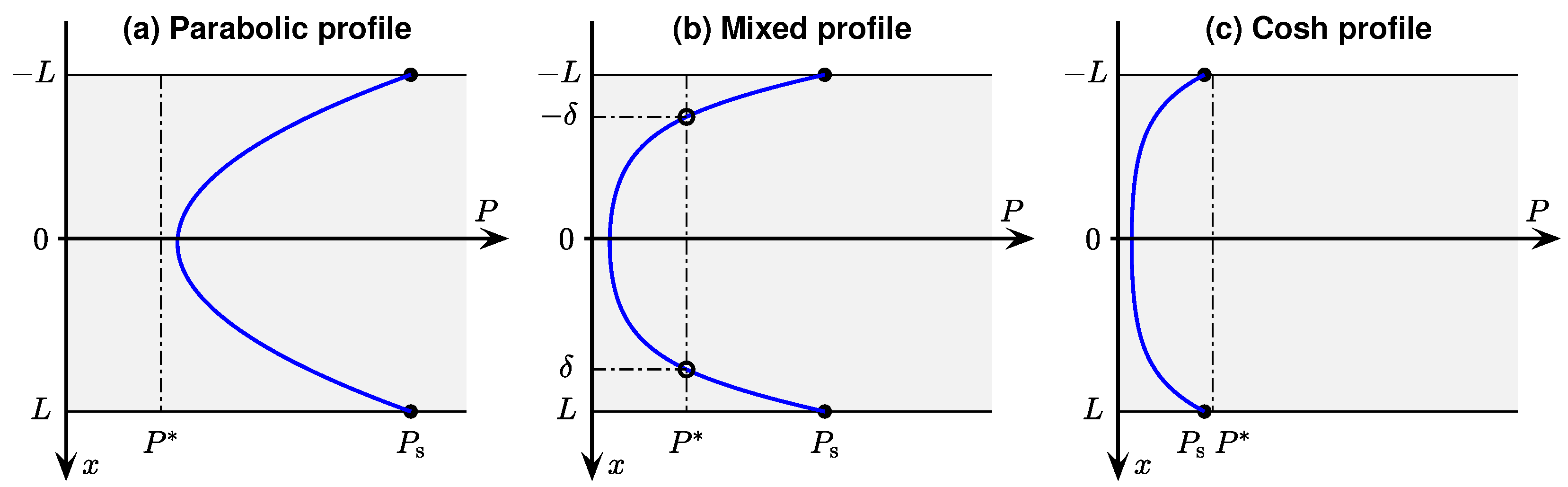
Q, the rate of oxygen consumption per unit volume of tissue. By selecting an idealised piecewise-linear model for consumption rate (
Section 2.2), the differential equation can be solved exactly. In
Section 2.3, we list the Ivanova & Simeonov [
10] solutions for three distinct boundary conditions, but choose here to work with dimensioned quantities, and to show explicitly the mirror symmetry of the
P vs.
x solutions about the slice central axis at
. In
Section 2.4, we demonstrate the validity of these solutions via optimised curve fits to four representative oxygen profiles obtained from cortical slices sustained in our perfusion bath (described later in
Section 3.1).
Section 2.5 surveys the surprisingly wide range of non-SI but ‘biologically convenient’ units used for Krogh coefficient in the literature, and comments on the potential ambiguity that can arise for unit conversions involving
, the molar volume of oxygen. In
Section 2.6, we use literature sources to investigate the temperature dependence of the Krogh coefficient of pure water, then consider the effect on
of adding salts and glucose to create aCSF, the artificial cerebrospinal fluid. We conclude the theoretical discussion in
Section 2.7 by describing how the tissue Krogh coefficient
can be determined via flux conservation across the tissue–fluid boundary.
Materials and Methods (
Section 3) details how the slices of brain tissue are prepared and sustained with a steady flow of oxygenated aCSF in the perfusion bath (
Section 3.1).
Section 3.2 describes the experimental setup that allows dual-hemisphere recording of both LFP (local-field potential) electrical activity and oxygen-tension variation with depth using a pair of oxygen probes co-located with the LFP wire electrodes. Our standard protocol (
Section 3.3) is to measure oxygen tension as a vertical profile, with soundings taken every 50
m through the fluid and tissue. The resulting pO
pressure profiles are processed using custom-written
Matlab software (
Section 3.4) to locate the slice centre, then extract the (
) curvature via iterative curve fitting. If a stationary fluid layer is detected, then the Krogh ratio
can be determined, and hence an estimate for
for a given pO
profile.
We present our results in
Section 4 for a range of fluid flow rates. The statistics for our
determinations show a large scatter about the mean value. By using pairs of repeated profiles at the same tissue location, we are able to distinguish natural biological variability from true experimental uncertainty. Our results suggest that, when comparing profiles from different locations within the same slice, natural variability in tissue Krogh coefficient is about three times larger than experimental errors arising from measurement uncertainty, curve fitting, and boundary gradient calculations. In
Section 5, we discuss our findings, and compare our results with Krogh coefficient values reported by other workers. We acknowledge limitations in our experimental approach, and make suggestions for future work.
3. Materials and Methods
In this section, we describe the experimental setup to measure pO profiles in thin slabs of mouse cortical tissue, and outline the software techniques used to analyse the profiles to extract curvatures and Krogh ratios.
3.1. Tissue Preparation
The brain was rapidly dissected from adult male and female C57 mice anaesthetised with CO
, then submerged in ice-cold ‘Normal’ artificial cerebrospinal fluid (aCSF); see
Table 3 for chemical composition. Coronal 400
m-thick sections were sliced between +1 to −5 Bregma using a vibrotome (Campden Instruments Ltd., Sileby, Leics, UK). The slices were then immersed at room temperature in no-magnesium (no-Mg) aCSF (see
Table 3, columns 4–6). All solutions were made in double-distilled water and pre-oxygenated (95% oxygen, 5% nitrogen) using an oxygen concentrator (Perfecto2, Invacare, Auckland, New Zealand) prior to use.
3.2. Data Recording
At least 60 min after preparing the tissue, the slices were transferred one at a time to a submersion-style perfusion bath based on a design by Thomas [
24] (see
Figure 5), and continuously perfused with aCSF. This design of the perfusion bath allows each hemisphere of the slice to be treated independently, but in this study both halves of the slice were exposed to identical experimental conditions. The aCSF flow rate was set at 0.5 mL/min for the repeated-profile experiments; flow values used in other experiments were [1, 2, 10] mL/min. Our expectation was that lower aCSF flow rates might favour the formation of a stationary boundary layer, but recognised that lower flows would restrict
supply and could compromise tissue function.
Slices were perfused throughout with no-Mg aCSF. Removing magnesium from the aCSF unblocks NMDA receptors [
25], resulting in the generation of ongoing spontaneous bursts of paroxysmal neuronal activity known as seizure-like events (SLEs) [
26]; these fast voltage transients provide a convenient and sensitive indicator of tissue viability, and allow correlation of neurophysiological activity with tissue-oxygen profile characteristics.
SLEs were detected using a 75 m diameter Ag/AgCl wire electrode inserted into the 400 m-thick tissue slice, and measured as an extracellular local-field potential difference developed between active tissue and a common-ground electrode (Ag/AgCl disc) placed some distance from the slice in the perfusion bath. The analog signal was amplified (1000×) and filtered (bandpass 1–100 Hz, notch filter at 50 Hz) (Model 3000 differential amplifier, A-M Systems, Sequim, WA, USA), then digitised at 1000 s (PowerLab, ADInstruments, Bella Vista, NSW, Australia) and recorded using LabChart 7 (ADInstruments, Australia).
Figure 5.
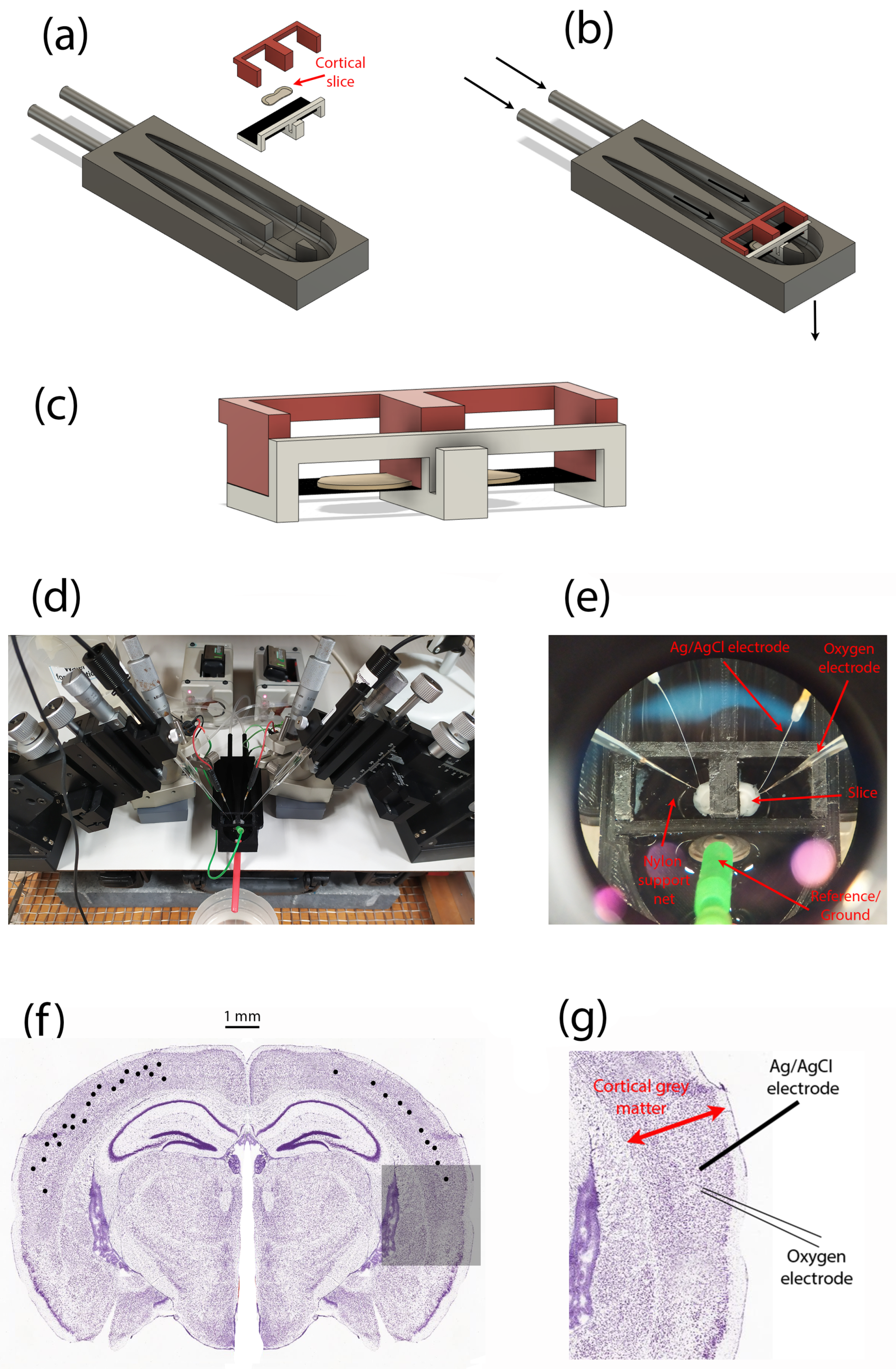
Perfusion bath and experimental setup for measuring oxygen-pressure profiles within a thin slice of mouse cortical tissue. (a) Exploded CAD model showing the separate components of the dual-compartment slice perfusion apparatus. (b) Assembled perfusion bath; arrows indicate direction of solution flow. (c) Enlarged view of the brain slice (grey ‘pancake’ shape) and its support structures; the slice sits on a nylon net (shown as a black-shaded horizontal surface). (d) Overview of experimental setup showing left and right pairs of micromanipulators, local-field potential (LFP) electrodes, oxygen probes. (e) Zoomed view of in situ cortical slice sitting on nylon net, and probed by LFP (Ag/AgCl wires) and oxygen (glass) electrodes. (f) Distribution of recording locations (black dots) within the slice cerebral cortex. For illustrative purposes, locations are shown on a single slice (but slices anterior to the one shown were used in some cases). Repeat profiles captured from some locations are not differentiated. (g) Representative arrangement of LFP electrode and oxygen probe for a single recording location, expanded from the shadowed region in (f).
Figure 5.
Perfusion bath and experimental setup for measuring oxygen-pressure profiles within a thin slice of mouse cortical tissue. (a) Exploded CAD model showing the separate components of the dual-compartment slice perfusion apparatus. (b) Assembled perfusion bath; arrows indicate direction of solution flow. (c) Enlarged view of the brain slice (grey ‘pancake’ shape) and its support structures; the slice sits on a nylon net (shown as a black-shaded horizontal surface). (d) Overview of experimental setup showing left and right pairs of micromanipulators, local-field potential (LFP) electrodes, oxygen probes. (e) Zoomed view of in situ cortical slice sitting on nylon net, and probed by LFP (Ag/AgCl wires) and oxygen (glass) electrodes. (f) Distribution of recording locations (black dots) within the slice cerebral cortex. For illustrative purposes, locations are shown on a single slice (but slices anterior to the one shown were used in some cases). Repeat profiles captured from some locations are not differentiated. (g) Representative arrangement of LFP electrode and oxygen probe for a single recording location, expanded from the shadowed region in (f).
![Ijms 24 06450 g005]()
Oxygen partial pressures (pO) were measured using a Clark-style oxygen electrode (50 m tip diameter, Unisense Ltd., Aarhus, Denmark) inserted into the tissue slice. Prior to experiments, the oxygen electrode was polarised to ensure a stable output signal, then two-point calibrated using (a) aCSF equilibrated with room air (pO = 160 mmHg), and (b) a solution of 0.1-M sodium ascorbate (zero-point). The pO data were sampled at ∼4.8 Hz using SensorTrace (v1.8, Unisense Ltd., Denmark).
3.3. Experimental Protocol
Once the slice was established in the perfusion bath, the Ag/AgCl wire electrode was inserted into layer III/IV of the cerebral cortex, with no specific cortical region targeted. If robust SLE activity was detected at that location (indicating viable tissue), the oxygen sensor was positioned using a precision micromanipulator (FX-117, Minitool Inc., Los Gatos, CA, USA) as close as practicable to the Ag/AgCl electrode, placing the tip of the oxygen probe in the bath fluid about 200 m above the slice surface.
The pO
vertical profile was recorded every 50
m by lowering the oxygen probe in 50-
m steps downwards through the upper fluid layer, then through the full depth of the 400-
m tissue slab, continuing until the tip had penetrated ∼100
m beyond the lower slice surface into the lower fluid layer. It was essential to include
soundings in the upper and lower fluid layers for two reasons. First, because of lack of visual contrast, it was not possible to accurately discern when the probe entered or exited the tissue, so the locations of the slice centre (
) and slice boundaries (
) could only be determined later, during the curve-fitting stage, by assuming that the curve minimum marked the (zero-flux) centre of symmetry. Second, we were seeking evidence of a nonflowing boundary layer in order to apply the flux-conservation argument of Equation (
19); this would manifest as an abrupt change in profile gradient on crossing the tissue–fluid boundary as the
P vs.
x profile curve transitions from parabolic to linear.
Some profiles exhibited a smooth tissue–fluid boundary crossing similar to those shown in
Figure 3, so were not suitable for estimation of tissue Krogh coefficient. In contrast,
Figure 6a,b,d display a clear gradient discontinuity at the lower tissue–fluid interface, but no gradient break at the upper interface. We attribute this profile asymmetry to a design characteristic of the slice perfusion system: the finely-woven nylon netting on which the slice sits (see
Figure 5c,e) seems to support the formation a locally static fluid layer immediately adjacent to the lower surface of the slice, without impeding the bulk flow of solution below the net. If the fluid is static (i.e., no advection), then oxygen transport through the fluid layer adjacent to the slice is via diffusion only; therefore, diffusive flux through the layer should match that entering the tissue, so the Equation (
19) assumption of flux conservation should be applicable here.
The fact that the probe detects a lower-surface stagnant layer in many—but not all—profiles suggests that the emergent location of the probe tip relative to the weave structure of the netting may be significant, but this aspect remains unresolved at present.
3.4. Numerical Methods and Curve Fitting
Each pressure profile consists of a vector of ∼20 oxygen tension readings [mmHg] recorded at 50-m intervals during a micromanipulator-controlled vertical descent starting in the fluid above the slice, then stepping down through the fluid into the tissue slice, through the slice, then continuing for several steps beyond the tissue into the fluid beneath. Tissue thickness is m, so either 8 or 9 samples will lie within the tissue. The precise position of the oxygen probe tip relative to the tissue boundary is not easily visualised, so the metabolic centre of the slice is determined mathematically by fitting a parabola to the profile: the pressure minimum locates the zero-flux reference depth .
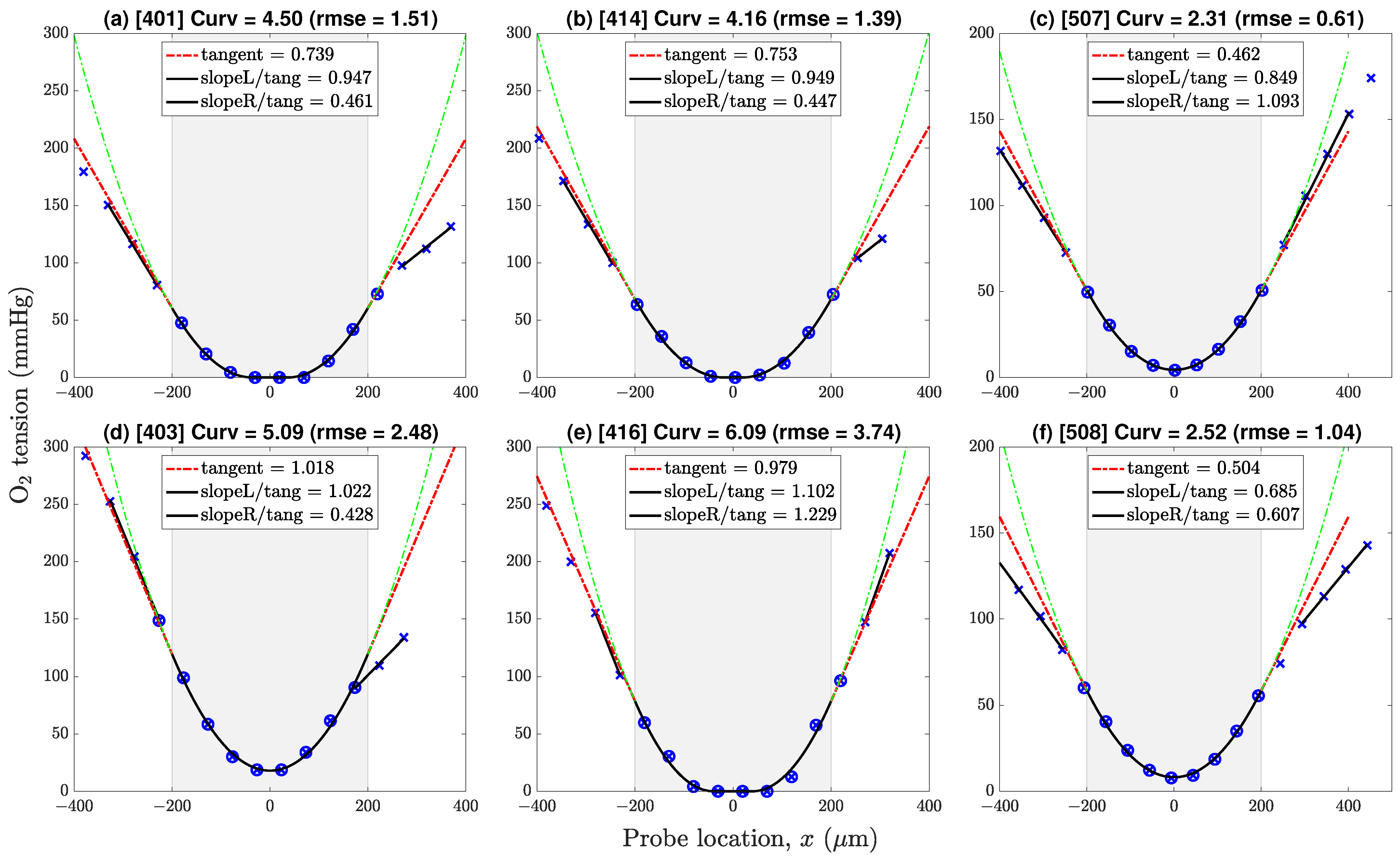
Figure 6.
Representative pressure profiles drawn from datasets v4 (first two columns) and v5 (third column). Profiles (a,b,d,f) show a gradient discontinuity at the lower boundary; profiles (c,e) do not. Negative/positive locations correspond to points lying above/below the line of symmetry. Key: × = sample values; ⊗ = samples selected for 9-point in-tissue curve-fit (parabola or paracosh); dashed-green = extrapolation of parabola/paracosh curve into fluid layers above (left) and below (right) the tissue–fluid interface; dashed-red = tangent to curve at boundary with slope [mmHg/m]; solid-black linear segments identify linear pressure trends in proximal fluid layer; ‘Curv’ = × curvature = × [mmHg/m]. Gradient ratios ‘slopeL/tang’, ‘slopeR/tang’ give estimates for above-slice, below-slice Krogh ratios; ratios exceeding cutoff value 0.725 are rejected.
Case (a): If the profile shape is accurately modelled as parabolic, then Equation (
20) applies, and the oxygen pressure gradient in tissue is given by
Case (b): If the pressure curve is ‘flat-bottomed’, then Equations (9) and (10) apply, indicating that the profile is a ‘paracosh’ mixed case with a hyperbolic-cosine (cosh) core for (
), and parabolic wings for (
). Paracosh fitting proceeds by iterating curvature
and critical pressure
to maximise agreement between the paracosh curve and the subset of
data points lying within the tissue boundaries. Paracosh optimisation makes use of
Matlab function fminsearchbnd [D’Errico (2022),
www.mathworks.com/matlabcentral/fileexchange/8277-fminsearchbnd-fminsearchcon, (accessed 29 June 2022)] which adds bounded constraints to the standard fminsearch optimiser; in our case, we require that both
and
be non-negative. The critical depth
is obtained via a separate iteration on Equation (
11) with surface pressure
fixed by linear interpolation of the
data pairs bracketing the
boundaries. Once the paracosh curve parameters
have been established, the pressure gradient at the
boundary is given by Equation (
25).
Case (c): The cosh-only profile () was never encountered in any of our oxygen tension soundings; nevertheless, the case-(b) curve-fitting algorithm should work equally well here.
If a clear gradient break could be identified at the tissue–fluid boundary, a straight line was fitted to the linear pressure trend in the fluid adjacent to the slice edge. The tissue–fluid Krogh ratio
was then obtained using the flux conservation expression of Equation (
24).
4. Results
We analysed five distinct pO profile datasets [labelled v1 to v5] but discarded the first two because of oxygen-probe calibration issues. The remaining datasets are:
Dataset v3 (10 mL/min): Recorded from 19 cortical locations from 4 slices (1 animal); profiles
Dataset v4 (1 and 2 mL/min): Recorded from 8 locations from 4 slices (1 animal), repeated at 1 and 2 mL/min for each location; profiles
Dataset v5 (0.5 mL/min): Recorded from 6 cortical locations from 2 slices (1 animal), each profile repeated once, giving 6 profile pairs; profiles
This gave a total of 47 oxygen tension profiles as summarised in
Table A1. Most of the curves (31 of 47) were well-fitted with a simple parabola; the remainder (16 of 47) were fitted with a mixed paracosh function (identified with ‘Flat = 1’ table entry); none of the profiles exhibited a purely cosh shape. The proportion of flattened curves decreased as aCSF flow rate was reduced: [42%, 31%, 25%] for [v3, v4, v5], respectively. Provided that each curve was correctly classified as parabolic or paracosh, we found no discernible difference between
estimates derived from the parabolic set compared with the paracosh set.
4.1. Oxygen Tension Profiles in Fluid and Tissue
Figure 6 shows six representative profiles with pressure gradient discontinuities evident at neither, one, or both tissue–fluid boundaries at
, slice half-thickness being
m. If the adjacent fluid exhibited a linear
trend, we took this as evidence of a local nonflowing fluid layer which should permit estimation of the (
) Krogh ratio via conservation of
flux across the interface (see Equation (
24)).
For each
pressure profile, Krogh ratio retrievals proceed via two independent curve-fitting steps. First, the optimal value of profile curvature
is determined by minimising the rms difference between measured
data points and iterated
parabola/paracosh predictions for the eight or nine locations
lying within the
tissue boundaries. The resulting pressure gradient at the boundary
is then calculated using Equation (
21) (parabola) or Equation (
25) (paracosh): see red ‘tangent’ extrapolations in
Figure 6.
Second, the pressure values in the proximal fluid above and below the slice are inspected for linear trends
, whose slope is markedly
lower from the tissue tangent extrapolations; a clear gradient break suggests a locally stationary fluid layer. For our experimental setup, these gradient breaks were common at the lower interface (at
), but rarely occurred at the top interface (
), except at the lowest perfusion rates. We attribute this top/bottom—left/right on the graphs—asymmetry to the presence of the fine nylon mesh that supports the underside of the slice (see
Figure 5); evidently, the weave of the net can create a ‘shadow zone’ that shields the slice from longitudinal advective currents.
If the fluid pressure gradient was similar to, or larger than, the extrapolated tissue gradient (i.e., if
), then the candidate ratio was immediately rejected (no stationary layer, therefore flux conservation assumption is invalid). However, a more stringent acceptance criterion is needed since some apparently stationary cases may be ‘contaminated’ by weak residual advective flows. After inspecting scatter plots of Krogh ratio vs. curvature (see
Figure 7 and
Figure 8a), and Krogh ratio histograms for
(
Figure 9), we set the ratio cutoff at
This selection was made on the basis that candidate Krogh ratios evidently fall into two clusters:
4.2. Scatter Plots of Krogh Ratio vs. Curvature
Individual scatter distributions for
candidate Krogh ratios vs. profile curvature are displayed as separate panels in
Figure 7, then aggregated into a unified cluster-graph in
Figure 8a;
Figure 8b shows the apparently sigmoidal dependence of profile curvature on perfusion flow rate. The scatterplots of
Figure 7 are segregated by interface (upper/lower) and by dataset (v3/v4/v5). Perfusion rates decrease from left to right: 10 mL/min (v3), 1 or 2 mL/min (v4), 0.5 mL/min (v5). We see that, on average, lower flow rates are associated with lower curvatures (‘flatter’ parabolic/paracosh curves). Since curvature =
, then
consumption rate also scales down as
supply becomes more restricted (assuming
can be taken as a nominal constant). In contrast, flow rate appears to have no influence on
plausible Krogh ratios (i.e., those that fall below the proposed 0.725 cutoff). These contrary sensitivities to fluid
transport rates are summarised in
Table 4.
The distribution of candidate Krogh ratios within a given dataset (v3/v4/v5) appears qualitatively rather noisy and erratic, unlike the curvature distributions. This is particularly evident in the paired observations in v4 and v5. For v4, each slice location was profiled twice, first at perfusion rate 1 mL/min, then at the doubled rate 2 mL/min. For every pair, doubling the flow rate raised the curvature by a roughly similar proportion; however, the impact on Krogh ratio was unpredictable and scattered (e.g., see outlier pair 414/416 in
Figure 7e), particularly for those candidate Krogh ratios lying in the nominated rejection zone. We attribute this increased scatter to three possible sources:
Krogh ratio requires separate tissue and fluid curve fits, so variance in the ratio will be the sum of the individual curve-fitting variances for tissue and fluid gradients;
the flux conservation argument used to derive Equation (
24) is invalid if the proximal fluid layer is not stationary (hence the need to impose a Krogh ratio cutoff);
formation of a local stagnant layer is not guaranteed, even within the closely woven structure of the nylon net that supports the slice.
We note that reducing the flow rate increases the proportion of candidate Krogh ratios that lie within our nominal acceptance range (i.e.,
), particularly for the lower interface (see bottom row of
Figure 7). Evidently, stagnant layer formation is more probable at low flow rates.
Table 4.
Sensitivity of profile curvature and Krogh ratio to variations in aCSF flow rate. Column headings identify the datasets used for computing statistics; the v4-dataset is partitioned into its high- and low-flow subsets. Perfusion rates decrease from left to right across the columns. Krogh statistics summarise the
(lower interface) retrievals, but note that candidate Krogh ratios that exceed the
cutoff have been excluded (see
Table A1).
| | v3 | v4 (hi) | v4 (lo) | v5 | All |
|---|
| Flow (mL/min) | 10.0 | 2.0 | 1.0 | 0.5 | |
|---|
| Curvature, | | | | | |
| 6.55 | 5.02 | 4.23 | 3.14 | |
| 1.38 | 0.85 | 0.80 | 0.90 | |
| N | 19 | 8 | 8 | 12 | |
| Krogh ratio, | | | | | |
| mean | 0.553 | 0.595 | 0.538 | 0.568 | 0.562 |
| stdev | 0.083 | 0.140 | 0.082 | 0.072 | 0.088 |
| N | 11 | 5 | 5 | 9 | 30 |
Figure 7.
Distribution of Krogh ratios as a function of curvature of fitted parabolic/paracosh function. Results are clustered by dataset (three columns: v3/v4/v5) and interface (two rows: upper/lower). Dashed-red horizontal marks the selected cut-off between accepted (below red line) and rejected (above line) Krogh ratios. Scanning from left to right, lower aCSF flow rates are generally associated with reduced curvature values, implying increasingly constrained
consumption. Linked pairs show repeated sampling at the same location. For v4, flow rate was set at 1 (open circles) or 2 mL/min (filled circles); for v5, flow rate was fixed at 0.5 mL/min. Outlier pairs 414/416 (v4) and 507/508 (v5) have very discrepant Krogh ratio estimates at the lower interface, possibly due to mechanical disturbance of the slice during withdrawal of
probe prior to repeat sounding. See
Figure 6 and
Table A1.
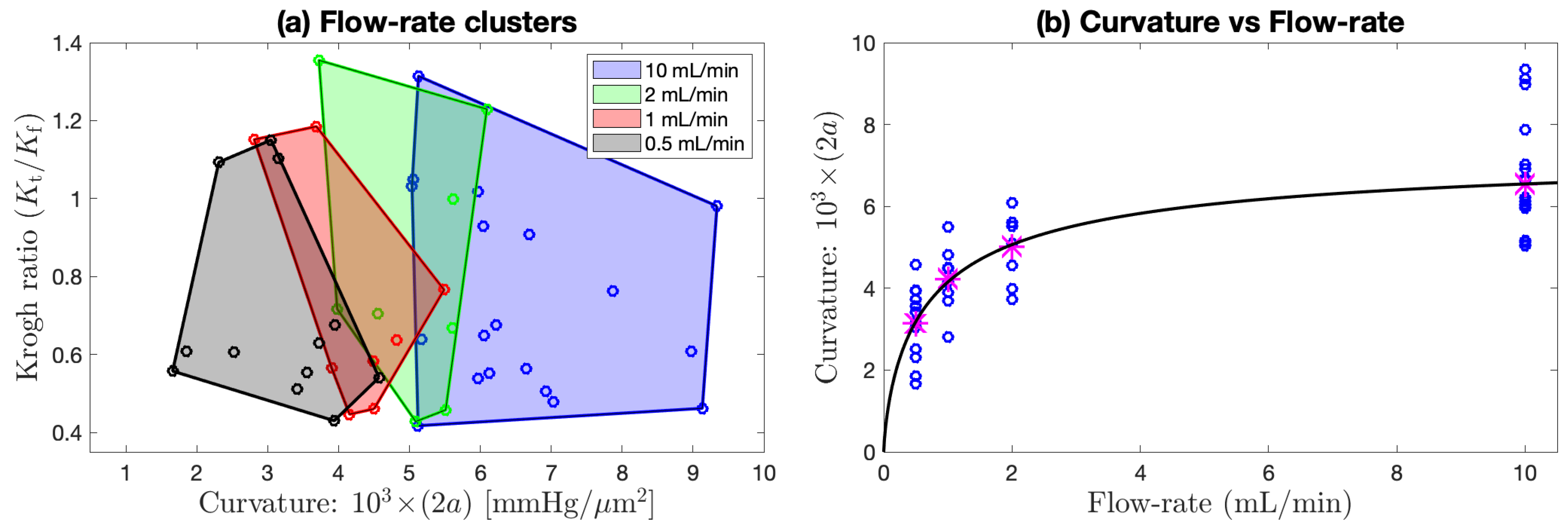
Figure 8.
Flow rate clustering and curvature dependence aggregated across (lower interface) of
Figure 7d–f. (
a) Aggregated scatterplot of candidate Krogh ratio
vs. curvature of fitted parabolic/paracosh function, clustered by flow rate [10, 2, 1, or 0.5] mL/min, as indicated by shaded convex-hull polygons (computed via
Matlab function convhull). Qualitatively, the polygon centroids move to the left as flow rate decreases, implying that curvature decreases (profiles become flatter) as perfusion flow rate is reduced. This trend is made quantitative in (
b) with a sigmoid fit to the
Table 4 curvature means (magenta asterisks) at each flow rate. The fitted curve is
with [
mmHg/
m
;
mL/min;
].
Unlike the v4 pairs, the perfusion rate for the v5 paired observations (
Figure 7c,f) was maintained at a constant value (0.5 mL/min); consequently, the profile repeats typically have smaller Cartesian separation (the links are smaller) than is the case for v4, and the average link length can be taken as an overall measure of the experimental uncertainty associated with our method. Nevertheless, we still see an outlier pair 507/508 at the lower interface with an abrupt reduction in the candidate Krogh ratio. While the 507/508 profile graphs in
Figure 6c,f show consistent in-tissue curvature values, the proximal fluid environment immediately above and below the tissue changes dramatically in the ∼1 min between the 507 and 508 soundings: the later profile shows clear evidence of stationary fluid layers at the upper and lower boundaries, while no evidence was apparent in the earlier profile. Perhaps the withdrawal and reinsertion of the
probe caused a subtle change in the seating of the tissue slab that favoured the formation of stagnant zones?
4.3. Histograms for Krogh Ratio and Profile Curvature
In
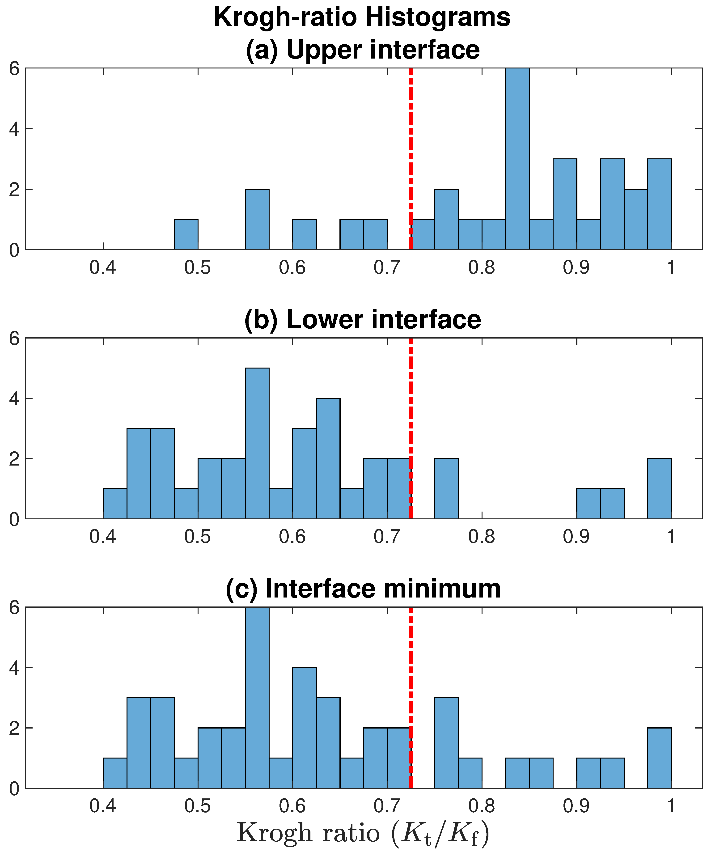
Figure 9, we present histograms for Krogh ratios aggregated over the [v3, v4, v5] datasets shown in
Figure 7, but restrict the analysis to
[allowing
would imply that
permeability in tissue
exceeds that in fluid; this is physiologically implausible]. Krogh ratios are biased towards larger values at the upper tissue–fluid interface (
Figure 9a), and smaller values at the lower interface (panel (b)); this is consistent with our observation that well-defined stagnant layers are a common occurrence at the lower boundary, but rare at the upper boundary. Setting an upper bound of
provides a clean separation between accepted and rejected Krogh ratio candidates.
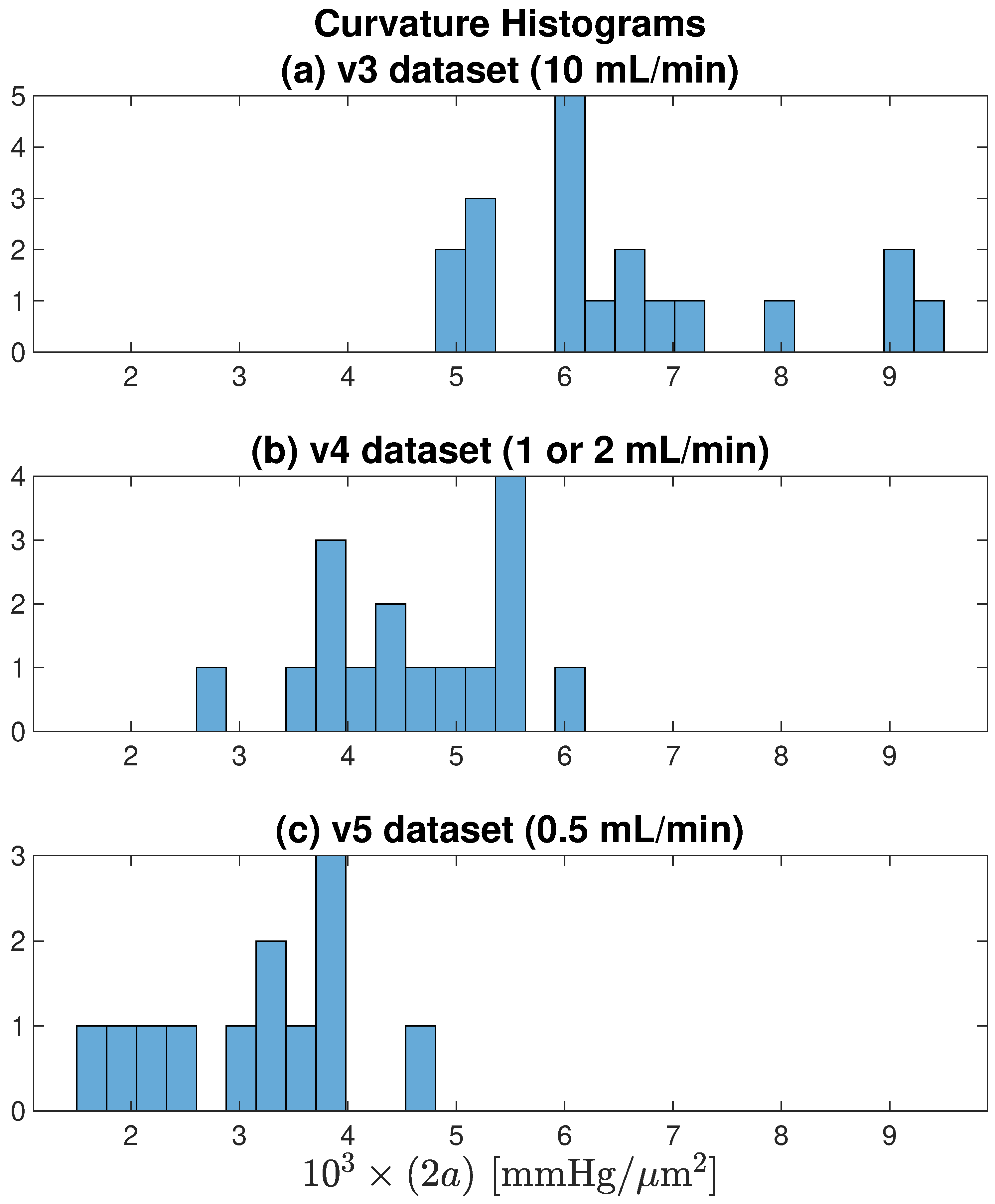
Figure 10 histograms the profile curvatures across each of the [v3, v4, v5] datasets. It confirms the earlier observation that smaller aCSF flow rates are associated with tissue profiles that have weaker (flatter) curvature, indicating that restricting oxygen flow leads to constrained metabolic activity.
Figure 9.
Histograms for Krogh ratios aggregated over [v3, v4, v5] datasets illustrated in
Figure 7, but restricted to domain
. Red-dashed line marks the accept/reject boundary set at 0.725: only Krogh ratios below cutoff are associated with a well-defined stationary layer. Comparing panels (
a,
b), the lower tissue–fluid interface is more likely to form a nonflowing boundary layer. In panel (
c), for each profile, the smaller of the [upper interface, lower interface] Krogh ratio is selected.
4.4. Possible Linkage between SLE Activity and Formation of Stationary Boundary Layer
We postulated that detection of a stagnant fluid layer at the tissue–fluid interface might require the maintenance of at least a minimum level of metabolic activity within the tissue. The ‘stationary fluid’ idealisation requires that—close to the tissue surface—oxygen diffusion (a molecular random walk with net motion directed towards the face of the tissue) through the fluid strongly dominates any residual advective bulk flow ( in fluid moving parallel to the tissue). However, if the tissue is not drawing much oxygen from the fluid, then diffusive flux across the interface will be low, and the advective component may no longer be insignificant, meaning that the flux conservation argument fails because the local fluid layer is insufficiently ‘stationary’.
Figure 10.
Curvature histograms for each of the [v3, v4, v5] datasets illustrated in
Figure 7. As flow rate decreases from (
a) 10 → (
b) [1 or 2] → (
c) 0.5 mL/min, average curvature decreases, meaning that the parabolic/paracosh curves become ‘flatter’ with shallower wings. For fixed
, a flatter curvature implies reduced metabolism.
We chose to test this hypothesis on the v3-database since this used the fastest aCSF flow rate (10 mL/min), thus maximising both delivery and the potential for seizure-like electrical activity. For each of the nineteen pressure soundings, we identified four consecutive seizure-like events (SLEs) that occurred around the time of profile acquisition, and computed average values for three SLE parameters: peak-to-peak amplitude [V]; duration [s]; inter-event frequency [s].
We found that SLE amplitude (but not SLE duration or frequency) correlated negatively with Krogh ratio for the under-slice interface (, ). That is, a tissue location generating smaller SLEs was less likely to display the pressure-gradient discontinuity associated with a nonflowing fluid layer at the boundary. Conversely, a site generating larger SLEs was more likely to show evidence of a stationary fluid layer.
4.5. Estimation of Krogh Coefficient for Cortical Tissue at Room Temperature
We now have sufficient data to derive an estimate for
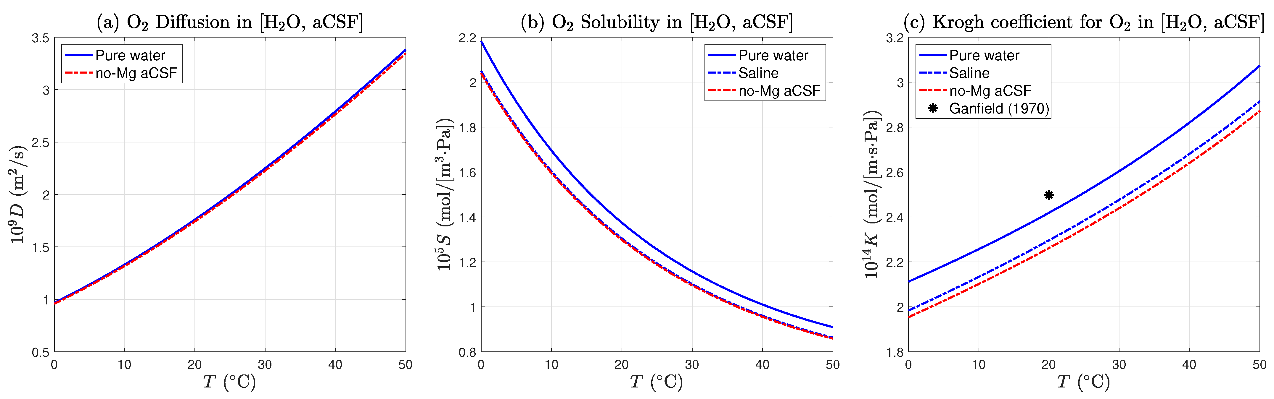
, the oxygen Krogh coefficient for mouse cortical tissue at room temperature. In
Section 2.6, we computed a theoretical value for
, the Krogh coefficient for the no-Mg aCSF (no-magnesium artificial cerebrospinal fluid) used to supply oxygen and glucose to the 400
m-thick slice of brain tissue (
18),
This value is based on that for pure water, but adjusted for the presence of dissolved salts and glucose. As displayed in
Figure 4, the coefficient is weakly temperature dependent. If the aCSF temperature were to rise from 20 to 25
,
would increase by ∼4% from [2.262 to 2.348] ×10
mol/[m·s·Pa]. We have chosen the middle of the range, with an uncertainty of ±2%.
From the
Table 4 statistics for the tissue–fluid ratio of Krogh coefficients
, we learn that the Krogh ratio is completely insensitive to perfusion rate, so we are justified in combining all datasets (last column of
Table 4) to give an aggregate (mean ± standard deviation) statistic,
The standard deviation in the ratio is ∼16% of the mean. This uncertainty estimate is almost an order of magnitude larger than the 2% relative uncertainty in for the perfusion fluid, so the latter can be neglected as source of uncertainty in the Krogh ratio. How much of this uncertainty is due to experimental error (e.g., probe calibration and positioning, pressure measurement, in-tissue and in-fluid curve fitting, tissue movement, unsteady flow rates, degraded stagnant layer, etc.), and how much arises from the natural variability of living cortical tissue?
The [v4, v5] repeated profiles—shown as linked pairs in
Figure 7e,f—allow us to apportion the relative contributions of experimental and biological sources of variation. There are eight linked pairs (four in each of [v4, v5]) that lie entirely within the
acceptance zone. Let
represent the (first, second) elements of the eight pairs of Krogh ratios retrieved at each repeated location. Define the biological and experimental contributions to the variance (i.e., square of the standard deviation) of the Krogh ratios as
and
, respectively. Then, the following variance identities should apply,
Our pairwise variance calculations give
implying that
of the variance in our Krogh ratio determinations is biological in origin, and the remaining 26% is attributable to experimental uncertainty.
Finally, we compute the room temperature Krogh coefficient for mouse cortical tissue by taking the product of (
27) and (
28),
where we have carried forward the 16% uncertainty from (
28).
5. Discussion
In this paper we have sought to provide a theoretical and experimental basis for determining oxygen consumption in thin slices of mouse brain tissue. Oxygen consumption within metabolically active tissue can be deduced from the curvature of pO
oxygen profiles using Fick’s law of diffusion, so long as the oxygen diffusion and solubility coefficients of tissue are known. Because oxygen solubility in tissue is difficult to measure, it is standard practice to work with the Krogh coefficient
, a lumped measure of oxygen permeability given by the product of diffusion and solubility coefficients for oxygen. Early work by Buerk & Saidel [
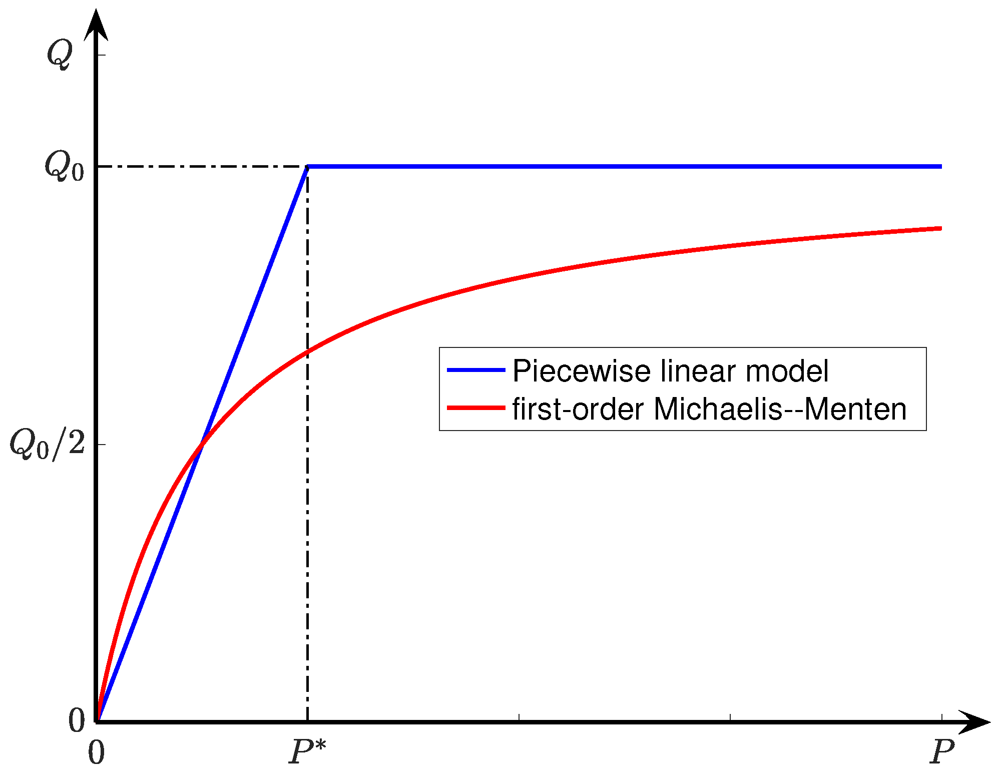
27] identified the Michaelis–Menton kinetics model as the most accurate description of pO
gradients in tissue slices; its piecewise-linear approximation (see Equation (
6)) provides the basis of the analytical solution published by Ivanova & Simeonov [
10] and extended here. We followed Ganfield et al. [
8] in assuming the existence of a narrow but stationary (i.e., non-flowing) boundary layer of fluid in close proximity to the tissue surface, then invoking conservation of oxygen flux across the fluid/tissue interface in order to deduce a value for
, the dimensionless ratio of tissue–fluid Krogh coefficients. By construction, the perfusion fluid is a passive, non-biologically active medium, so the fluid Krogh coefficient
can be calculated from well-established interpolation formulas that are functions of both water temperature and saline concentration; this then allows tissue Krogh coefficient
to be determined.
There are alternative ways to measure the tissue Krogh coefficient experimentally; however, these are generally not appropriate for soft, delicate tissue such as brain. For example, the original gaseous diffusion method described by Krogh (1919) [
16] involved separating two chambers with a stretched membrane, allowing measurement of gas diffusion through the membrane from one chamber to the other. A similar direct measurement method was applied by Sasaki et al. [
14], using microscopy techniques to measure the flux of oxygen across thin (10–20
m) arteriolar walls. Such methods are not easily applied to a slice of brain tissue since it is very easily damaged by physical manipulation.
It is informative to compare our value for tissue Krogh coefficient with those published in the literature. This requires appropriate unit conversions from SI to the various alternative unit systems in use. We select two of the more common metric choices:
| (mL O2)/(cm·min·atm): | | Ganfield et al. [8] |
| (mmol O2)/(cm·min·mmHg): | | Ivanova & Simeonov [10] |
and list the unit-remapped values for our estimate for
,
Using the second set of units (), Ganfield et al. (1970) derive a Krogh coefficient for cat cortex of , about 27% lower than our estimate. Their result is unexpectedly low, given that they were working at 37 , while our value was derived at room temperature.
Ivanova & Simeonov (2012) tabulate a range of Krogh coefficients at 37 for a variety of different tissues drawn from the work of several authors. Using the third set of units (), their quoted values for covered the range
0.59 (kidney), 0.65 (liver), 1.35 (brain), 1.44 (heart),
so our value of 1.03 × 10 for mouse cortex is certainly plausible, given the temperature difference.
We have focused on calculating tissue/fluid Krogh ratio in the first instance. The advantage of working with a dimensionless ratio is that it should aid direct comparison between studies since it eliminates the need for non-SI unit conversions. Although the biological significance of expressing Krogh permeability as a ratio is uncertain, it is plausible that the ratio may be less sensitive to temperature than either component. If so, this would be advantageous when attempting to compare the findings of different research groups working with a range of perfusion temperatures. This idea remains to be tested experimentally.
Our method for computing the Krogh ratio is dependent of the formation of a stationary boundary layer at the tissue–fluid interface. As discussed previously, a nonflowing fluid layer was often detected at the lower interface, but rarely at the upper interface. This asymmetrical behaviour is probably a favourable artifact created by the support netting on which the slice sits: it seems that the tight weave of the netting can provide shielding from the bulk advective flow. This likely explains some of the variability in our estimate, because precise positioning of the oxygen electrode within this stationary layer could not be guaranteed from one recording location to the next.
Importantly, when (repeat) profiles were collected from the same location, the variance in the ratio was substantially lower (contributing only 26% of the total variation), indicating that the majority of the variability was of biological origin. This hints at the possibility that the oxygen permeability characteristics of brain tissue are not uniform across and between slices, with potential influences from variation in cortical layer structure, variation in regional cortical anatomy, and spatial differences in tissue viability. In these experiments, we did not attempt to control for specific cortical anatomical location or for non-uniformity in slice viability.
In summary, we have found that the Ivanova & Simeonov diffusion–consumption model provides an excellent description of oxygen-tension distribution within a thin slice of active tissue. We have extended the model to include the effects of a stationary fluid layer at the boundary, and have shown how to compute the ratio of tissue and fluid Krogh coefficients via a flux conservation argument. Being dimensionless, the Krogh ratio allows unambiguous and direct comparisons between studies by different researchers, since it obviates the need for unit conversions. The mapping to dimensioned Krogh coefficients can be delayed until the choice of units for the fluid Krogh coefficient has been made.


