
Comparison of SPEED, S-Trap, and In-Solution-Based Sample Preparation Methods for Mass Spectrometry in Kidney Tissue and Plasma

 , , , , , and
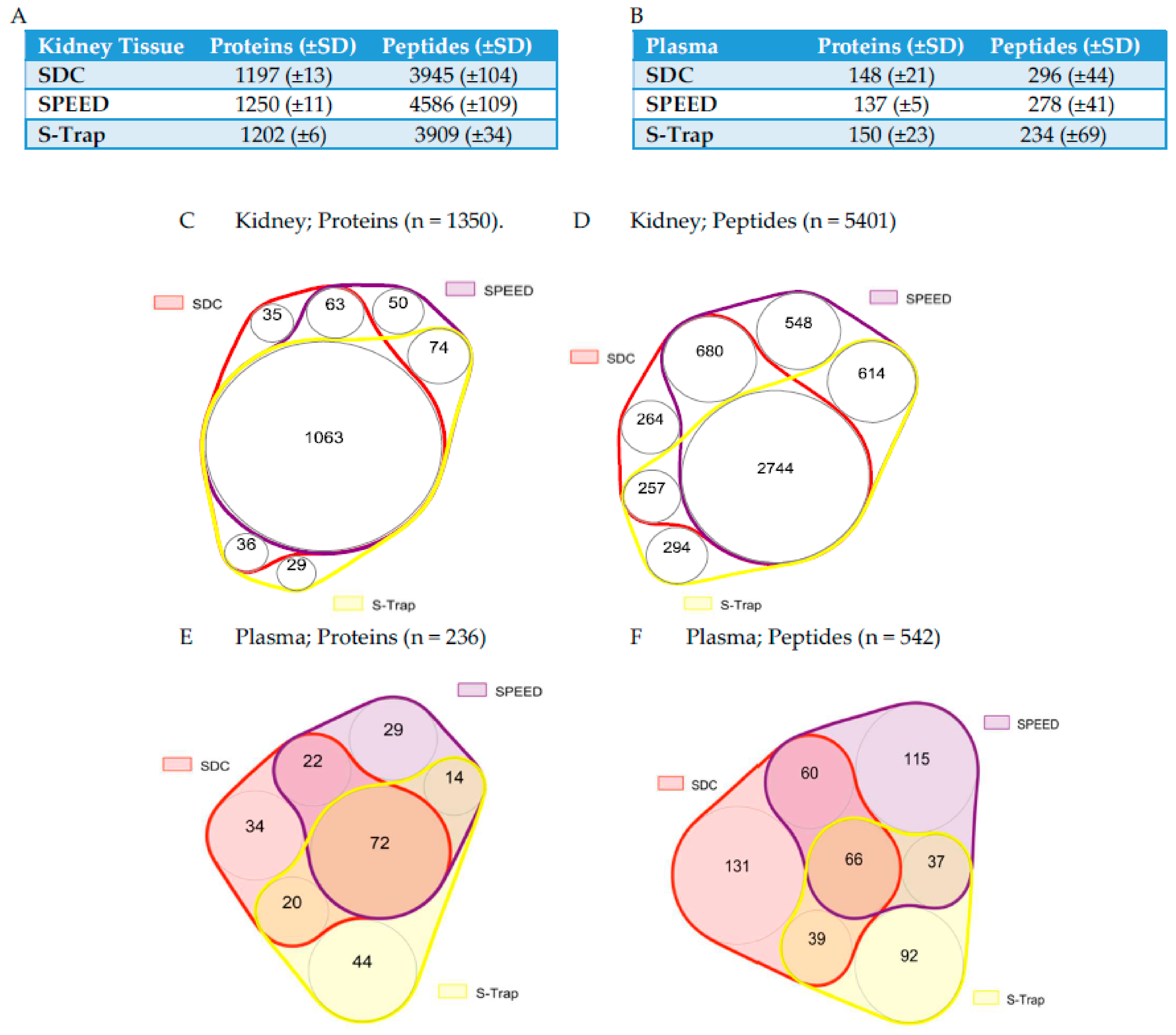
Abstract
:1. Introduction
2. Results and Discussion
2.1. Protein and Peptide Quantification Using SWATH
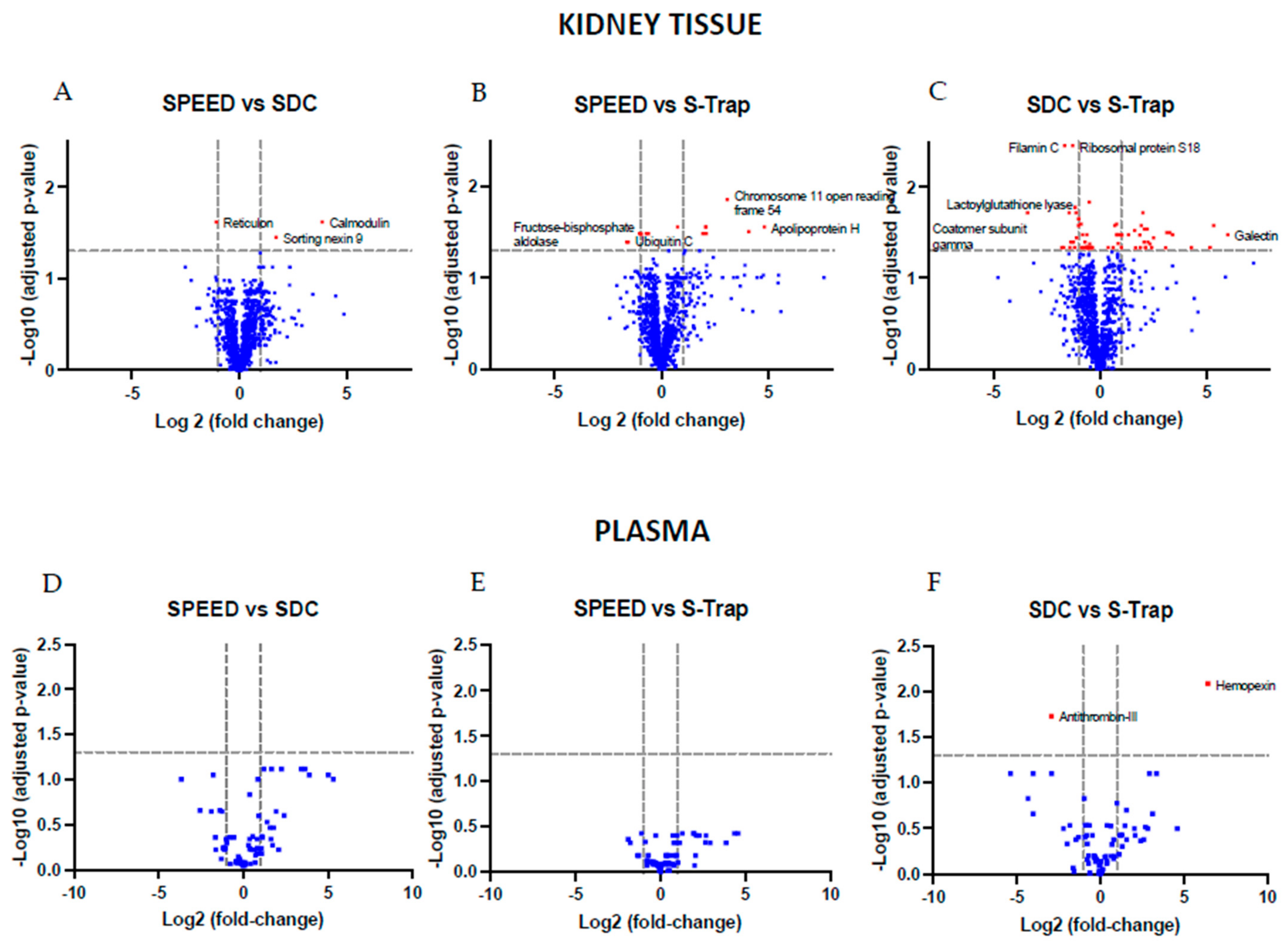
2.2. Comparing Quantifications across Methods
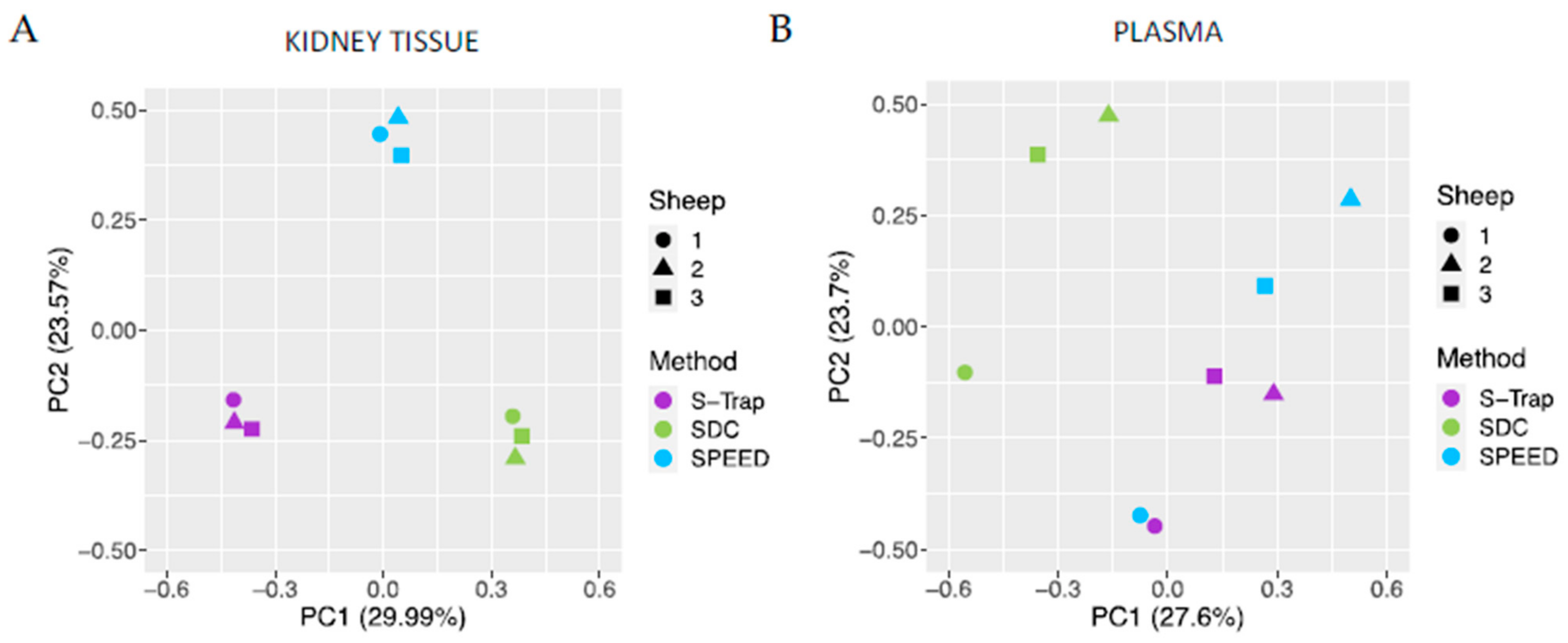
2.3. Reproducibility of SWATH Quantifications
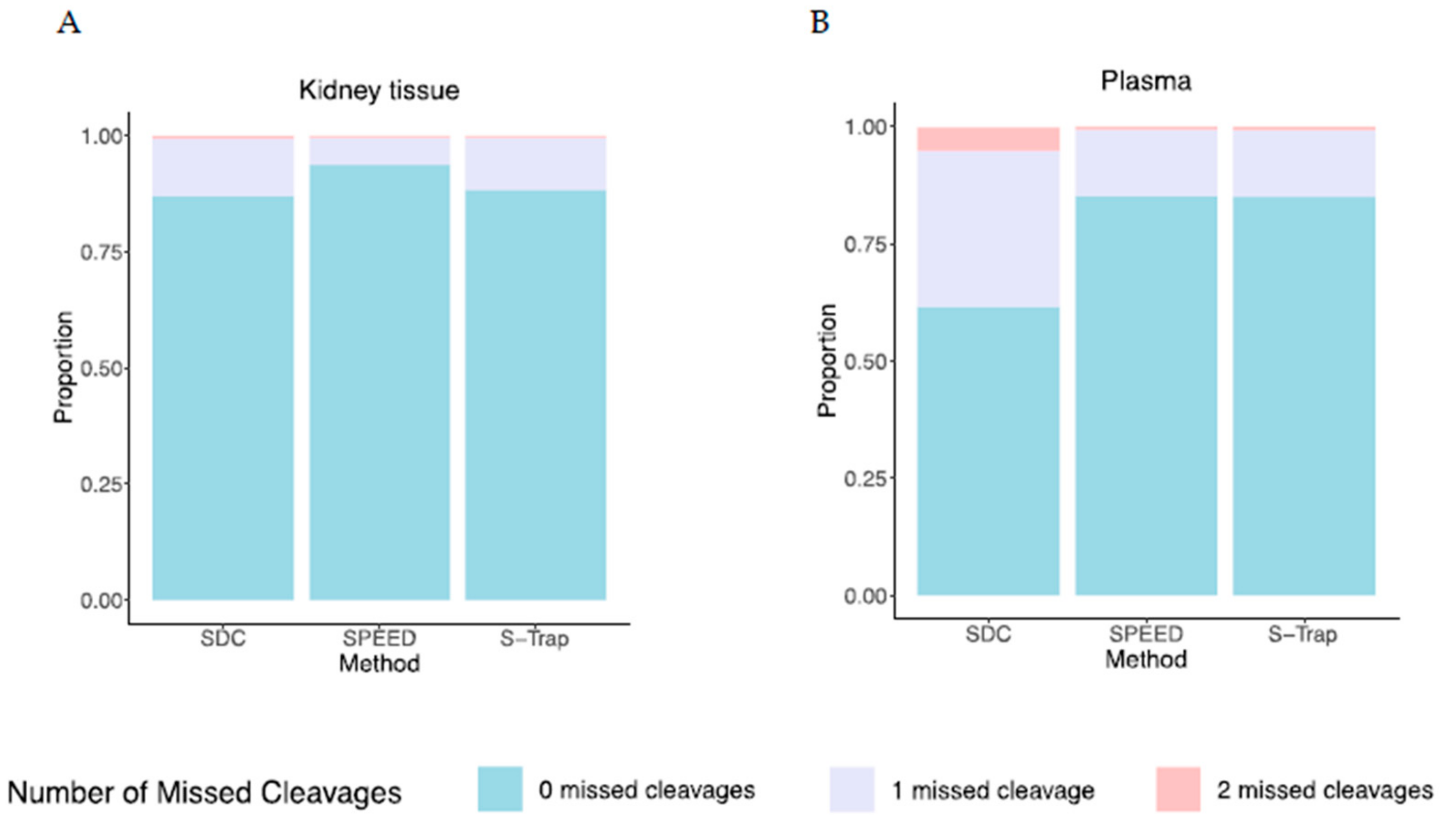
2.4. Efficiency of Proteolysis
2.5. Physical Characteristics
2.6. Practical Considerations
2.7. Limitations
3. Conclusions
4. Materials and Methods
4.1. Animals
4.2. Sample Preparation
4.2.1. SPEED
4.2.2. S-Trap
4.2.3. SDC
4.2.4. Desalting Peptides
4.3. Data-Dependent and SWATH Mass Spectrometry
4.4. Data Analysis
4.4.1. DDA Data Quality Assessment Using SearchGUI
4.4.2. Spectral Library Build Using ProteinPilot
4.4.3. SWATH Data Analysis
4.4.4. Quality Control of SWATH Data
4.5. Statistical Analysis
Supplementary Materials
Author Contributions
Funding
Institutional Review Board Statement
Data Availability Statement
Acknowledgments
Conflicts of Interest
References
- Aslam, B.; Basit, M.; Nisar, M.A.; Khurshid, M.; Rasool, M.H. Proteomics: Technologies and Their Applications. J. Chromatogr. Sci. 2017, 55, 182–196. [Google Scholar] [CrossRef] [PubMed] [Green Version]
- Crutchfield, C.A.; Thomas, S.N.; Sokoll, L.J.; Chan, D.W. Advances in mass spectrometry-based clinical biomarker discovery. Clin. Proteom. 2016, 13, 1. [Google Scholar] [CrossRef] [PubMed] [Green Version]
- Rinschen, M.M.; Saez-Rodriguez, J. The tissue proteome in the multi-omic landscape of kidney disease. Nat. Rev. Nephrol. 2020, 17, 205–219. [Google Scholar] [CrossRef]
- Dubin, R.F.; Rhee, E.P. Proteomics and Metabolomics in Kidney Disease, including Insights into Etiology, Treatment, and Prevention. Clin. J. Am. Soc. Nephrol. 2020, 15, 404–411. [Google Scholar] [CrossRef] [PubMed] [Green Version]
- Gregorich, Z.R.; Chang, Y.H.; Ge, Y. Proteomics in heart failure: Top-down or bottom-up? Pflugers Arch. 2014, 466, 1199–1209. [Google Scholar] [CrossRef] [Green Version]
- Leon, I.R.; Schwammle, V.; Jensen, O.N.; Sprenger, R.R. Quantitative assessment of in-solution digestion efficiency identifies optimal protocols for unbiased protein analysis. Mol. Cell. Proteom. 2013, 12, 2992–3005. [Google Scholar] [CrossRef] [Green Version]
- Ludwig, K.R.; Schroll, M.M.; Hummon, A.B. Comparison of In-Solution, FASP, and S-Trap Based Digestion Methods for Bottom-Up Proteomic Studies. J. Proteome Res. 2018, 17, 2480–2490. [Google Scholar] [CrossRef]
- Batth, T.S.; Tollenaere, M.A.X.; Ruther, P.; Gonzalez-Franquesa, A.; Prabhakar, B.S.; Bekker-Jensen, S.; Deshmukh, A.S.; Olsen, J.V. Protein Aggregation Capture on Microparticles Enables Multipurpose Proteomics Sample Preparation. Mol. Cell. Proteom. 2019, 18, 1027–1035. [Google Scholar] [CrossRef] [Green Version]
- Doellinger, J.; Schneider, A.; Hoeller, M.; Lasch, P. Sample Preparation by Easy Extraction and Digestion (SPEED)—A Universal, Rapid, and Detergent-free Protocol for Proteomics Based on Acid Extraction. Mol. Cell. Proteom. 2020, 19, 209–222. [Google Scholar] [CrossRef]
- Wisniewski, J.R.; Zougman, A.; Nagaraj, N.; Mann, M. Universal sample preparation method for proteome analysis. Nat. Methods 2009, 6, 359–362. [Google Scholar] [CrossRef]
- Hughes, C.S.; Foehr, S.; Garfield, D.A.; Furlong, E.E.; Steinmetz, L.M.; Krijgsveld, J. Ultrasensitive proteome analysis using paramagnetic bead technology. Mol. Syst. Biol. 2014, 10, 757. [Google Scholar] [CrossRef] [PubMed]
- Zougman, A.; Selby, P.J.; Banks, R.E. Suspension trapping (STrap) sample preparation method for bottom-up proteomics analysis. Proteomics 2014, 14, 1006–1000. [Google Scholar] [CrossRef] [PubMed]
- Duan, X.; Young, R.; Straubinger, R.M.; Page, B.; Cao, J.; Wang, H.; Yu, H.; Canty, J.M.; Qu, J. A straightforward and highly efficient precipitation/on-pellet digestion procedure coupled with a long gradient nano-LC separation and Orbitrap mass spectrometry for label-free expression profiling of the swine heart mitochondrial proteome. J. Proteome Res. 2009, 8, 2838–2850. [Google Scholar] [CrossRef] [PubMed] [Green Version]
- Klont, F.; Bras, L.; Wolters, J.C.; Ongay, S.; Bischoff, R.; Halmos, G.B.; Horvatovich, P. Assessment of Sample Preparation Bias in Mass Spectrometry-Based Proteomics. Anal Chem. 2018, 90, 5405–5413. [Google Scholar] [CrossRef] [Green Version]
- Choksawangkarn, W.; Edwards, N.; Wang, Y.; Gutierrez, P.; Fenselau, C. Comparative study of workflows optimized for in-gel, in-solution, and on-filter proteolysis in the analysis of plasma membrane proteins. J. Proteome Res. 2012, 11, 3030–3034. [Google Scholar] [CrossRef] [Green Version]
- HaileMariam, M.; Eguez, R.V.; Singh, H.; Bekele, S.; Ameni, G.; Pieper, R.; Yu, Y. S-Trap, an Ultrafast Sample-Preparation Approach for Shotgun Proteomics. J. Proteome Res. 2018, 17, 2917–2924. [Google Scholar] [CrossRef]
- Zhang, G.; Fenyo, D.; Neubert, T.A. Evaluation of the variation in sample preparation for comparative proteomics using stable isotope labeling by amino acids in cell culture. J. Proteome Res. 2009, 8, 1285–1292. [Google Scholar] [CrossRef] [Green Version]
- Piehowski, P.D.; Petyuk, V.A.; Orton, D.J.; Xie, F.; Moore, R.J.; Ramirez-Restrepo, M.; Engel, A.; Lieberman, A.P.; Albin, R.L.; Camp, D.G.; et al. Sources of technical variability in quantitative LC-MS proteomics: Human brain tissue sample analysis. J. Proteome Res. 2013, 12, 2128–2137. [Google Scholar] [CrossRef] [Green Version]
- Schmidt, I.M.; Sarvode Mothi, S.; Wilson, P.C.; Palsson, R.; Srivastava, A.; Onul, I.F.; Kibbelaar, Z.A.; Zhuo, M.; Amodu, A.; Stillman, I.E.; et al. Circulating Plasma Biomarkers in Biopsy-Confirmed Kidney Disease. Clin. J. Am. Soc. Nephrol. 2022, 17, 27–37. [Google Scholar] [CrossRef]
- Bhawal, R.; Oberg, A.L.; Zhang, S.; Kohli, M. Challenges and Opportunities in Clinical Applications of Blood-Based Proteomics in Cancer. Cancers 2020, 12, 2428. [Google Scholar] [CrossRef]
- Tanca, A.; Biosa, G.; Pagnozzi, D.; Addis, M.F.; Uzzau, S. Comparison of detergent-based sample preparation workflows for LTQ-Orbitrap analysis of the Escherichia coli proteome. Proteomics 2013, 13, 2597–2607. [Google Scholar] [CrossRef]
- Sielaff, M.; Kuharev, J.; Bohn, T.; Hahlbrock, J.; Bopp, T.; Tenzer, S.; Distler, U. Evaluation of FASP, SP3, and iST Protocols for Proteomic Sample Preparation in the Low Microgram Range. J. Proteome Res. 2017, 16, 4060–4072. [Google Scholar] [CrossRef]
- Katz, J.J. Anhydrous trifluoroacetic acid as a solvent for proteins. Nature 1954, 174, 509. [Google Scholar] [CrossRef]
- Rademaker, M.T.; Pilbrow, A.P.; Ellmers, L.J.; Palmer, S.C.; Davidson, T.; Mbikou, P.; Scott, N.J.A.; Permina, E.; Charles, C.J.; Endre, Z.H.; et al. Acute Decompensated Heart Failure and the Kidney: Physiological, Histological and Transcriptomic Responses to Development and Recovery. J. Am. Heart. Assoc. 2021, 10, e021312. [Google Scholar] [CrossRef]
- Bennis, A.; Ten Brink, J.B.; Moerland, P.D.; Heine, V.M.; Bergen, A.A. Comparative gene expression study and pathway analysis of the human iris- and the retinal pigment epithelium. PLoS ONE 2017, 12, e0182983. [Google Scholar] [CrossRef]
- Dayon, L.; Kussmann, K. Proteomics of human plasma: A critical comparison of analytical workflows in terms of effort, throughput and outcome. EuPA Open Proteom. 2013, 1, 8–16. [Google Scholar] [CrossRef] [Green Version]
- Gundry, R.L.; White, M.Y.; Murray, C.I.; Kane, L.A.; Fu, Q.; Stanley, B.A.; Van Eyk, J.E. Preparation of proteins and peptides for mass spectrometry analysis in a bottom-up proteomics workflow. Curr. Protoc. Mol. Biol. 2009, 90, 10.25.1–10.25.23. [Google Scholar]
- Lasse, M.; Pilbrow, A.P.; Kleffmann, T.; Andersson Overstrom, E.; von Zychlinski, A.; Frampton, C.M.A.; Poppe, K.K.; Troughton, R.W.; Lewis, L.K.; Prickett, T.C.R.; et al. Fibrinogen and hemoglobin predict near future cardiovascular events in asymptomatic individuals. Sci. Rep. 2021, 11, 4605. [Google Scholar] [CrossRef]
- Leeman, M.; Choi, J.; Hansson, S.; Storm, M.U.; Nilsson, L. Proteins and antibodies in serum, plasma, and whole blood-size characterization using asymmetrical flow field-flow fractionation (AF4). Anal Bioanal Chem. 2018, 410, 4867–4873. [Google Scholar] [CrossRef] [Green Version]
- Vaudel, M.; Barsnes, H.; Berven, F.S.; Sickmann, A.; Martens, L. SearchGUI: An open-source graphical user interface for simultaneous OMSSA and X!Tandem searches. Proteomics 2011, 11, 996–999. [Google Scholar] [CrossRef]
- Craig, R.; Beavis, R.C. TANDEM: Matching proteins with tandem mass spectra. Bioinformatics 2004, 20, 1466–1467. [Google Scholar] [CrossRef] [PubMed] [Green Version]
- Elias, J.E.; Gygi, S.P. Target-decoy search strategy for mass spectrometry-based proteomics. Methods Mol. Biol. 2010, 604, 55–71. [Google Scholar] [PubMed] [Green Version]
- Apweiler, R.; Bairoch, A.; Wu, C.H.; Barker, W.C.; Boeckmann, B.; Ferro, S.; Gasteiger, E.; Huang, H.; Lopez, R.; Magrane, M.; et al. UniProt: The Universal Protein knowledgebase. Nucleic Acids Res. 2004, 32 (Suppl. 1), D115–D119. [Google Scholar] [CrossRef]
- Vaudel, M.; Burkhart, J.M.; Zahedi, R.P.; Oveland, E.; Berven, F.S.; Sickmann, A.; Martens, L.; Barsnes, H. PeptideShaker enables reanalysis of MS-derived proteomics data sets. Nat. Biotechnol. 2015, 33, 22–24. [Google Scholar] [CrossRef] [PubMed]
- Taus, T.; Kocher, T.; Pichler, P.; Paschke, C.; Schmidt, A.; Henrich, C.; Mechtler, K. Universal and confident phosphorylation site localization using phosphoRS. J. Proteome Res. 2011, 10, 5354–5362. [Google Scholar] [CrossRef]
- Vaudel, M.; Breiter, D.; Beck, F.; Rahnenfuhrer, J.; Martens, L.; Zahedi, R.P. D-score: A search engine independent MD-score. Proteomics 2013, 13, 1036–1041. [Google Scholar] [CrossRef]
- Barsnes, H.; Vaudel, M.; Colaert, N.; Helsens, K.; Sickmann, A.; Berven, F.S.; Martens, L. Compomics-utilities: An open-source Java library for computational proteomics. BMC Bioinform. 2011, 12, 70. [Google Scholar] [CrossRef] [Green Version]
- Wu, J.X.; Song, X.; Pascovici, D.; Zaw, T.; Care, N.; Krisp, C.; Molloy, M.P. SWATH Mass Spectrometry Performance Using Extended Peptide MS/MS Assay Libraries. Mol. Cell. Proteom. 2016, 15, 2501–2514. [Google Scholar] [CrossRef] [Green Version]
- Hunter, C. What Is the Best Strategy for Doing Retention Time Calibration When Doing SWATH Acquisition? Available online: https://sciex.com/community/application-discussions/proteomics/swath/data-processing/what-is-the-best-strategy-for-doing-retention-time-calibration-when-going-swath-acquisition (accessed on 12 November 2022).
- Bjelosevic, S.; Pascovici, D.; Ping, H.; Karlaftis, V.; Zaw, T.; Song, X.; Molloy, M.P.; Monagle, P.; Ignjatovic, V. Quantitative Age-specific Variability of Plasma Proteins in Healthy Neonates, Children and Adults. Mol. Cell. Proteom. 2017, 16, 924–935. [Google Scholar] [CrossRef] [Green Version]
- R Core Team R: A Language and Environment for Statistical Computing. Available online: https://www.R-project.org/ (accessed on 5 October 2022).
- R Studio Team. R Studio: Integrated Development for R. Available online: http://www.rstudio.com/ (accessed on 5 October 2022).
- Ludwig, C.; Claassen, M.; Schmidt, A.; Aebersold, R. Estimation of absolute protein quantities of unlabeled samples by selected reaction monitoring mass spectrometry. Mol. Cell. Proteom. 2012, 11, M111.013987. [Google Scholar] [CrossRef] [Green Version]
- Liu, Y.; Buil, A.; Collins, B.C.; Gillet, L.C.; Blum, L.C.; Cheng, L.Y.; Vitek, O.; Mouritsen, J.; Lachance, G.; Spector, T.D.; et al. Quantitative variability of 342 plasma proteins in a human twin population. Mol. Syst. Biol. 2015, 11, 786. [Google Scholar] [CrossRef]
- Niu, L.; Geyer, P.E.; Wewer Albrechtsen, N.J.; Gluud, L.L.; Santos, A.; Doll, S.; Treit, P.V.; Holst, J.J.; Knop, F.K.; Vilsboll, T.; et al. Plasma proteome profiling discovers novel proteins associated with non-alcoholic fatty liver disease. Mol. Syst. Biol. 2019, 15, e8793. [Google Scholar] [CrossRef]
- Osorio, D.; Rondon-Villarreal, P.; Torres, R. Peptides: A Package for Data Mining of Antimicrobial Peptides. Small 2015, 7, 4–14. [Google Scholar] [CrossRef]
- Tang, Y.; Horikoshi, M.; Li, W.X. Ggfortify: Unified Interface to Visualize Statistical Results of Popular R Packages. R. J. 2016, 8, 474–485. [Google Scholar] [CrossRef] [Green Version]


Disclaimer/Publisher’s Note: The statements, opinions and data contained in all publications are solely those of the individual author(s) and contributor(s) and not of MDPI and/or the editor(s). MDPI and/or the editor(s) disclaim responsibility for any injury to people or property resulting from any ideas, methods, instructions or products referred to in the content. |
© 2023 by the authors. Licensee MDPI, Basel, Switzerland. This article is an open access article distributed under the terms and conditions of the Creative Commons Attribution (CC BY) license (https://creativecommons.org/licenses/by/4.0/).
Share and Cite
Templeton, E.M.; Pilbrow, A.P.; Kleffmann, T.; Pickering, J.W.; Rademaker, M.T.; Scott, N.J.A.; Ellmers, L.J.; Charles, C.J.; Endre, Z.H.; Richards, A.M.; et al. Comparison of SPEED, S-Trap, and In-Solution-Based Sample Preparation Methods for Mass Spectrometry in Kidney Tissue and Plasma. Int. J. Mol. Sci. 2023, 24, 6290. https://doi.org/10.3390/ijms24076290
Templeton EM, Pilbrow AP, Kleffmann T, Pickering JW, Rademaker MT, Scott NJA, Ellmers LJ, Charles CJ, Endre ZH, Richards AM, et al. Comparison of SPEED, S-Trap, and In-Solution-Based Sample Preparation Methods for Mass Spectrometry in Kidney Tissue and Plasma. International Journal of Molecular Sciences. 2023; 24(7):6290. https://doi.org/10.3390/ijms24076290
Chicago/Turabian StyleTempleton, Evelyn M., Anna P. Pilbrow, Torsten Kleffmann, John W. Pickering, Miriam T. Rademaker, Nicola J. A. Scott, Leigh J. Ellmers, Christopher J. Charles, Zoltan H. Endre, A. Mark Richards, and et al. 2023. "Comparison of SPEED, S-Trap, and In-Solution-Based Sample Preparation Methods for Mass Spectrometry in Kidney Tissue and Plasma" International Journal of Molecular Sciences 24, no. 7: 6290. https://doi.org/10.3390/ijms24076290