2.2.1. Basic Network Elements
To describe the job landscape inside an organization, we distinguish between two types of entities, employed individuals (
) and the “location” of the employment (
) (the term location is not ideal, but other choices such as
class, used in the manpower literature [
22] are also problematic and thus we choose location because it better fits our analysis). Our data identify individuals as well as several possible choices of locations such as operating units within an organization, geographic locations (such as US States) where some part of the organization operates, or types of occupations that the organization requires (say, data analysts or accountants, recorded with a standardized code system [
21]). Here, we use the term location as a descriptor to indicate where the individual can be found within the organization. For example, if we are interested in knowing the movements of the workforce by geography,
i would represent a particular US state where some of the organization has facilities. On the other hand, if we want to know the distribution of the workforce by occupation,
i would be an occupational code.
Our characterization of the system is based on the structure of labor markets, which are studied by looking at the interrelated dynamics of individuals employed or looking for employment and the jobs those individuals occupy or the vacancies they may aspire to fill. In previous studies of LFNs, the choice of location was not discussed in itself, perhaps determined by the data available (e.g., in [
8,
10] only firms and employees are recorded, making locations represent firms). However, in our case, not only does the data provide an opportunity to explore several possibilities, but there is a genuine question about which choice of location to use in terms of better accuracy of the models, something we address below and return to in
Section 4.
Given a choice for
i, an Organizational Labor Flow Network (OLFN) is generated in the following way. Consider a set of individuals
and job locations
. We denote the sizes of the sets as
and
. The work histories of individuals, usually called
sequences in career studies, are typically recorded at discrete and uniformly distributed time points
, where
is the initial time of observation,
T the number of time units of observation (equal to the duration of the data) and, in our case, the units are in months. Thus, we define the
employment sequence of agent α by
where
i is a job location,
the first time
is observed to be in the organization, and
is the so-called job tenure (the number of time units an employee spends in the organization). Note that
and
and that information about individual starting and ending times is necessary to know given that many employees join and/or leave over a period of time.
The nodes of an OLFN are constituted by the job locations
. A link
between two nodes in the OLFN is possible only if there are job transitions from
i to
j, but this may not guarantee a link. Instead,
would be included as a link in the OLFN if statistically significant job transitions are observed between the nodes [
10]. The statistical test is explained in
Section 2.2.2.
2.2.2. Statistical Significance of Organizational Labor Flow Networks
An OLFN can be defined in several ways beyond the choice of locations, just as long as it leads to reliable networks in terms of forecasting future job change. This means that, to construct an OLFN, we must check that information gathered at some period of time can be used to forecast a subsequent time period. This requires that we statistically test the reliability of past information in terms of providing information about the future. But, how to design this test?
In this system, job changes past or future appear as job transitions. Thus, we must find a way to take information about transitions and convert this to links in a network. In other words, links may only be introduced between pairs of locations (nodes) that have had job transitions between them, although the final decision can depend on additional criteria (see below). Following on, we must further consider whether linking a node pair should be done independently or related to linking other node pairs. We can quickly realize that to choose links between node pairs independently of each other runs the risk of ignoring correlations. For example, some locations are characterized by many people (large operating units or popular occupation codes), while others by a few. For the case of a large location, it is likely that it sends and receives many workers, an effect that is felt across many of the node pairs that involve that node. This acts as a correlation between the large node and the transitions involving other nodes, effectively coupling its possible links. Therefore, it is generally more appropriate to decide on adding links by taking into account their correlated structure. The simplest way to do this would be to correlate links that connect to the same node, independent of other nodes. This approach, however, is likely to ignore higher order correlations that trickle through from node to node. Therefore, an even better strategy would be to decide on links on the basis of the whole network structure.
We must also choose a time frame with job transitions that help us predict future transitions. In this case, we pick a simple strategy that works well in that it provides proof of principle. Thus, we divide the data into two equal-size time periods, and , that we refer to respectively as and . The first time period acts as the baseline, whereas the second corresponds to the forecasting (or test) period. From the baseline period, we take transitions and consider them as candidates for links. The testing period is then used to determine whether our choices of links have been appropriate in terms of making our OLFN useful for prediction.
Having established time windows, we must decide how to introduce links. While an approach that would explore the entire space of possible combinations of linking in some designated period of time could be imagined, in practice this is very challenging due to the combinatorial explosion of possibilities. Instead, we take an approach related to [
7] but also addresses the fact that their method ignores the link correlations we identified above. In [
7], each pair of firms in the city of Stockholm is considered independently and a single transition between firms is used to gauge subsequent likelihood of transitions. Here, as in [
7], we adopt the notion that observing a transition between a node pair suggests they should be linked, but introduce a numerical threshold
representing the minimum number of transitions (in either direction) between two locations
i and
j in order to make that pair of nodes a
candidate to have a link. This generates a
candidate network where node pairs have tentative links if they satisfy the threshold.
The final step of the statistical test is to check if the candidate network is indeed predictive. To do this, we construct possible random future networks (meant to be in time period
) and compare them with information from the candidate network in the past (from time period
). Two pieces of information have been used in [
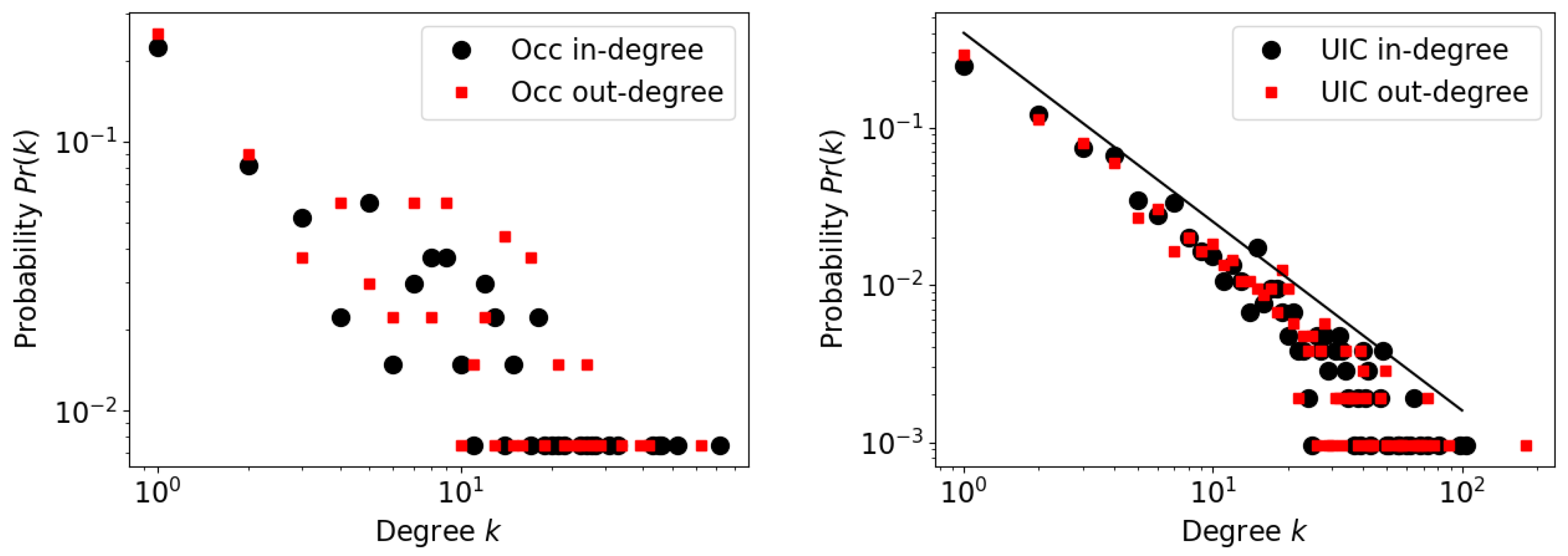
10] for this purpose. First, let us define
and
as, respectively, the number distinct nodes from which workers transition into node
i and the number distinct nodes to which workers transition to from
i, both within time period
. Similarly, we define
as the number of workers that transition from other nodes into
i over the period
, and
the number of workers that transition from
i to other nodes in the same period. These quantities are versions of the concepts of node degree and node strength [
23].
It was found in [
10] that the most demanding version of test was the one that preserved
and
because the statistic that measures the amount of deviation from random transitions produced the smallest (yet highly significant) results. To perform this test, we generate a large number of distinct realizations of random networks using Monte Carlo. Each such network is created by randomly assigning transitions between nodes in the period
while requiring that
and
remain true in each and every realization for all nodes. To generate a statistic, the random model lets us estimate an expectation value for how many transitions can randomly occur between a pair of nodes that is a candidate link, based on a given threshold
, from period
. Introducing the notation
for the set of candidate links during
and
for set of stochastic transitions predicted by each realization of one of the random models during
, all the null models generate an expected density of overlaps
which measures the expected fraction of candidate links from
that would also have a transition during
simply by random chance. In this expression, the customary notation of size of a set
and expectation
have been used. Clearly, the choice of stochastic model alters the resulting set
.
From the standpoint of observation, we want to know among the
, what fraction of them were observed to have transitions during
. Labeling the observed transitions as
, the fraction of transitions matching candidate links is given by
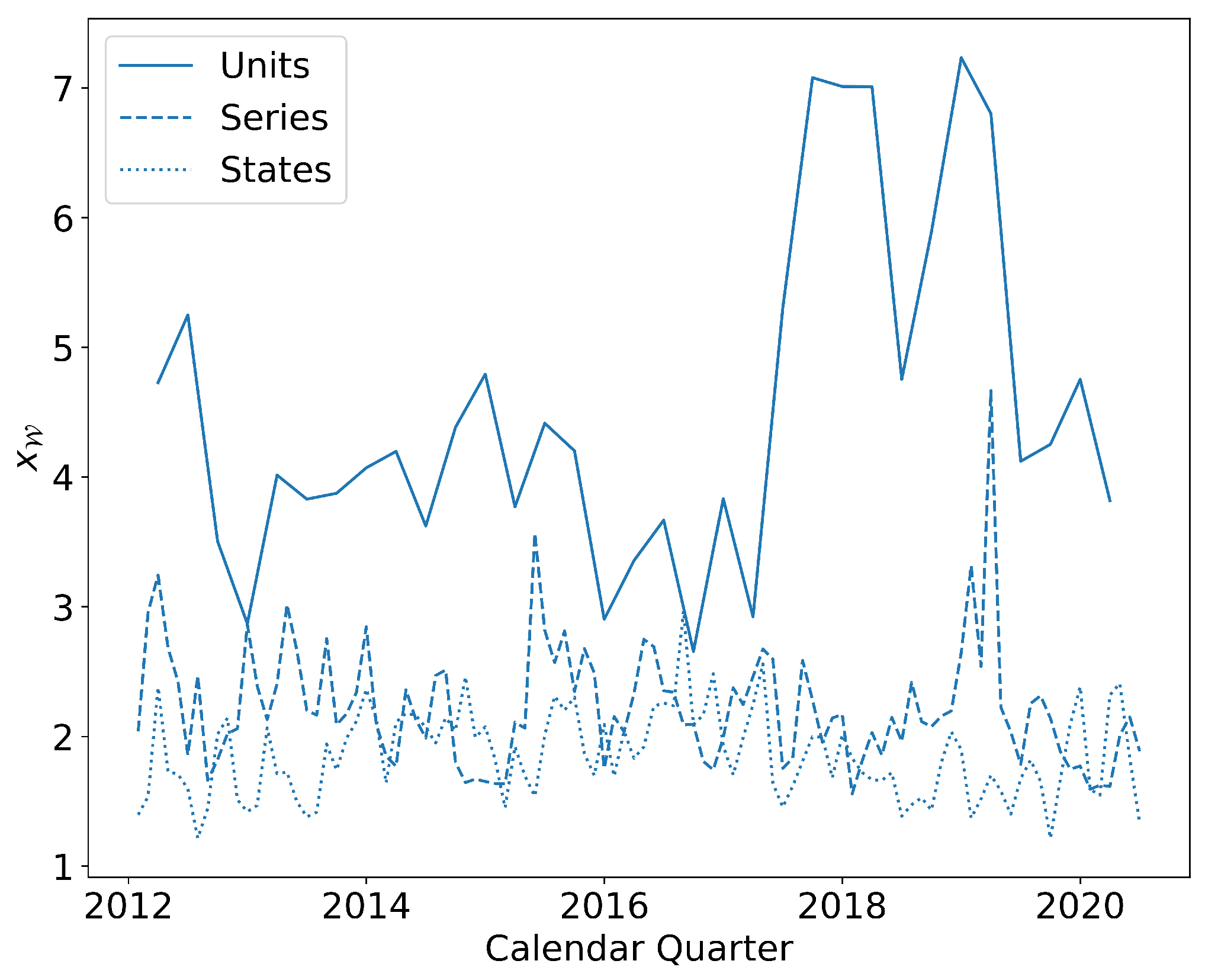
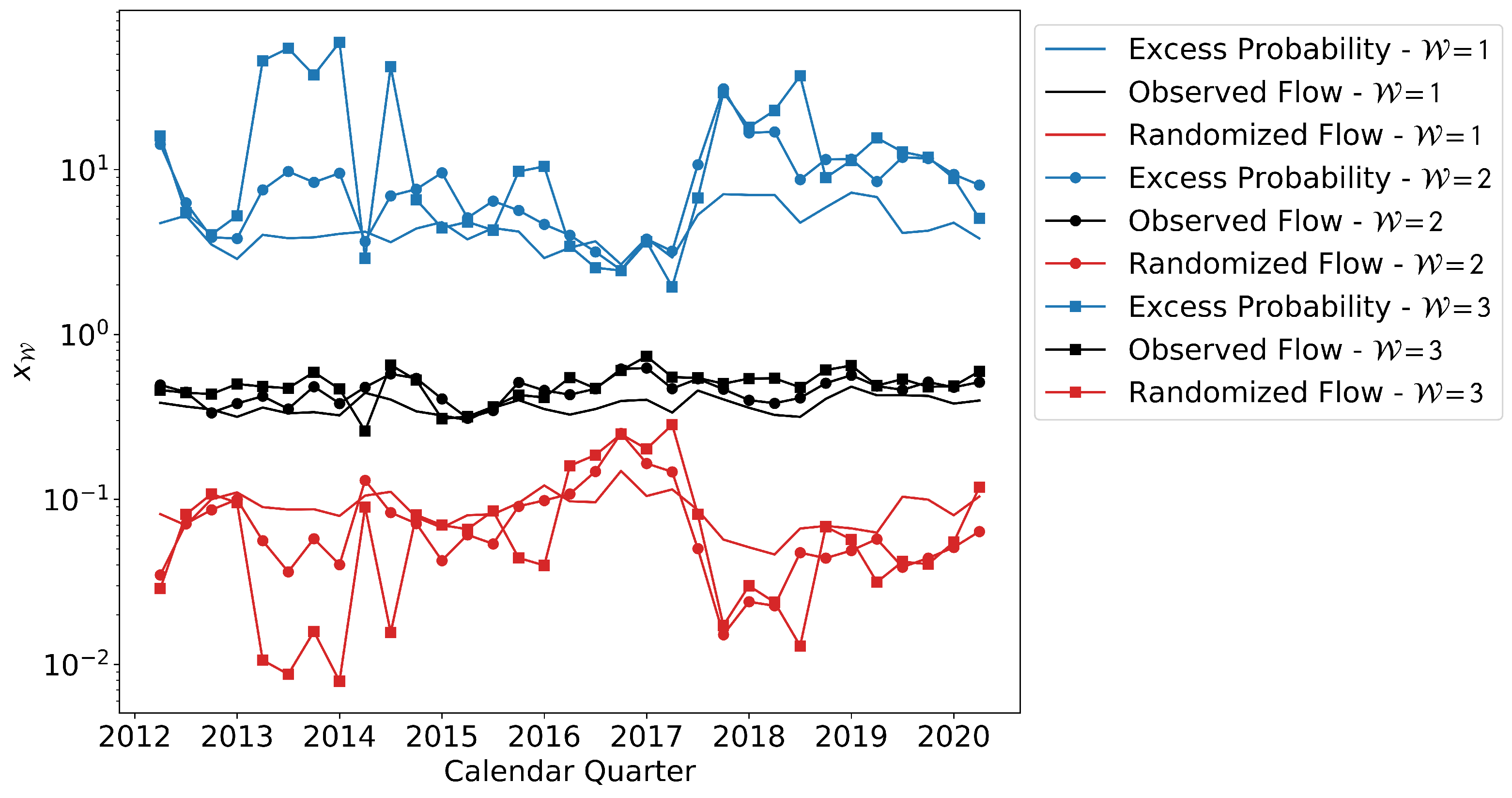
The statistic of interest is finally defined as the ratio between the two quantities, which we call the excess probability
, given by
If
is above 1 with a large degree of certainty (has a very small
p-value), we conclude that the threshold
leads to an OLFN that is useful for prediction. To provide intuition for this statement, note that
measures the network averaged increase in probability with respect to the random model that a transition during
occurs along a pair of nodes with
or more transitions during
. To illustrate, if
is 2, the transitions actually observed during
are twice as likely to occur along pairs of nodes that had
transitions during
than what would be expected from the random model. Therefore, a value of
(and the greater the better) means that transitions during
are predictable on the basis of transitions during
because they prefer to occur along candidate links by a factor of
than along random node pairs. Finally, as a technical point, the
p-values can be determined semi-analytically (or analytically in the case of the uncorrelated random model, where only the total number of system transitions is preserved) by using the methodology in [
10].
2.2.3. Career Sequences and Their Probability Distributions
To study careers, we are interested in the
non-degenerate version of the sequences encoded in Equation (
1). To illustrate what this means, consider an employment sequence
in which
spends from
t to
working at location
i, or
but
and
. We will refer to such a time period of uninterrupted work at a given location as a
spell.
Since our primary interest is in the locations (or career steps) individuals take, we create a non-degenerate version of called such that only the location of a spell is recorded but not the number of time steps spent in a location. Thus, for example, if ’s career is spent only in two locations, i and j and , the corresponding career sequence is . We should note that preserves temporal ordering so that if first worked in location i and then in j, these appear in that same order in . Our sequences also possess the feature that if an individual were to return to a previous location, this would be captured in the sequence. Thus, an individual with an employment sequence of the form would have career sequence .
The frequencies with which career sequences occur is very useful information because they offer insights on the sorts of choices individuals make under the constraints of the opportunities that become available within the organization (an individual cannot change into a job that is not offered, an important observation from the perspective of modeling made by the seminal work of White [
24]). In order to understand how common or rare specific career sequences are, we define the distribution of observed sequences
, where
is the random variable of career sequences. For a given time period of observation,
where
corresponds to the career sequence of
,
is the Kronecker delta equal to 1 when
’s career matches the desired sequence
u and 0 otherwise, and the denominator is the total number of distinct careers observed. Described intuitively, Equation (
5) precisely defines how we count careers to determine their probability of occurring.
Because careers can be sensitive to the initial location, we further specialize our analysis to distinguish careers on the basis of their initial location. Let us label the first location of career
u as
(or
when the career refers to that of individual
). Then, we are interested in the set of conditional distributions
2.2.5. Markov Models of Career Sequences
To test the usefulness of OLFNs in modeling the movement of personnel across an organization, we construct two Markov chains, one which relies solely on the network structure (based on [
9,
10]) and another that uses the network structure plus memory (when applicable) about the prior transition [
18]. At the most basic level, Markov chains require that one defines states of the system and probabilities to go between states. Our method based solely on network structure uses as states the current job (node) held by an employee, and the probability to transition between jobs is estimated on the basis of the transitions made by all workers over some selected period of time of the data (for example, the first half of the years in the data). On the other hand, our method to include memory generally defines as a state the tuple made of the current and previous job a worker has held (with exceptions needed to handle the first job of the worker), and the transition probabilities are estimated from other workers and the last two jobs they held. We now describe these details.
Let us start by clarifying that both models simply lead to the creation of simulated employment sequences and their associated career sequences. Since we mostly focus on career sequences, we introduce and to represent random career sequences respectively created from the Markov network model or the Markov model with one-step memory. These random variables are characterized by the distributions and . These distributions are created from a large number of model realizations. There are two kinds of such realizations. On the one hand, a single random walker can only generate a single career, not enough to generate useful distributions or . Therefore, to generate these distributions, we use walkers which correspondingly generate careers from which to create the distributions. A second way to introduce multiple realizations is to generate distributions and so that no one single realization of walkers dominates the results. Our ultimate goal is to determine the quality of the models, which we do by defining below a set of metrics that compare each of these distributions to .
A common feature to both models is the fact that individuals can begin to work at the organization at any time in any one of its locations. For the purposes of modelling their career sequences, one could ignore the specific point in time unless there were reasons to assume that temporal interactions play an important role. The initial location, on the other hand, is always relevant in terms of the number of either employment of career sequences generated. Thus, we should keep in mind that all the distributions we study are in reference to careers that start at each specific location (node) in the network.
One last feature shared by both models is that the number of time steps an individual travels is drawn from the length of service distribution . The effect is that each individual has a randomly drawn, fixed lifetime in the organization so that after time , the individual’s career sequence (either or ) is completed and counted toward the appropriate distribution.
The model based on [
10] makes use of the network structure but, deviating from that article, also includes weights to construct the transition rates between nodes. In the model, a simulated individual located at
i at time step
t has a probability
to choose
j as their next location, and this probability is constant in time. To determine
, we make use of all the employment sequences in Equation (
1). Such sequences can be used from the entire data (all the time points) or limited to parts of the time (e.g.,
which would require some small adjustments like redefining work spells). Assuming we are using the entire data, we first count the number of moves
from node
i to
j on the basis of the number of sequences (and the number of times in that sequence) where a transition occurs from
i to
j. Concretely,
This equation states that
is given by the number of times any individual makes a transition from
i to
j. For the Markov process, the probability of the transition
i to
j is then given by the proportion of all transition out of
i that go to
j with respect to all transitions out of
i, or
Note that the definitions of
and
include diagonal terms. Thus, the diagonal of the transition matrix of the Markov chain accounts for the very frequent occurrence of individuals remaining in their locations.
In contrast to the pure network model, the model that keeps track of the previous step (if the career has visited at least one other node) makes use of a slightly more complicated transition matrix. Note that when an individual enters the network at a node and has not yet made transitions to other nodes, the model is applied as if it was the pure network model described above; only after one transition can memory begin to play a role. To make use of memory, let us focus on a node
j. The probability that an individual transitions from
j to
h given that it had previously transitioned from
i to
j is based on the number of careers that have previously made the same sequence of moves. Therefore, if
is given by
the probability for an individual to go from
j to
h given that they came from
i is given by
In both types of models, it is possible that the probabilities are 0 for an individual to move beyond their current location. If that is the case, the individual merely remains in the node until either the simulation finishes or the number of time units assigned to the individual are complete. We should note that a single realization for a walker can last up to the length of time we choose to model.
2.2.6. Evaluating Predicted Career Sequences
Next, we describe the metrics we use to assess the quality of the models. Essentially, we are interested in knowing whether the models tend to produce with high probability the careers actually observed, along with their observed frequencies. Symbolically, this is equivalent to testing for the similarity of the numerical values between and when over the space of possibilities of u (the sample space), where for the memoryless Markov model or the one-step memory model, respectively. As a practical matter, we note that because all careers are distinguished by their initial location i, all the quantities we define are computed according to their initial location. Stated in plain English, the data show certain career paths and the models try to imitate these. Therefore, evaluating the models is done by checking how “similar” the imitation created by the models is to the observed careers.
In an ideal scenario, two distributions are similar if their sample spaces are similar and the probabilities of events (the elements of the sample space) are also similar. To be precise about what similar means, we now proceed to introduce several different quantitative measures of that similarity and highlight how each focuses on a particular aspect of that similarity.
Let us first concentrate on the similarity between probabilities
and
. In this case, similarity means that the observed and modeled probabilities of the same career
u starting at node
i have similar values, i.e.,
. But this comparison has to be done carefully because for any given initial node
i,
u is not independent of other careers starting from
i. Let us denote all the observed careers starting from
i as
. Then, they are related by the fact that
which is the normalization condition for
. Modeled careers also satisfy a similar relation; calling the set of these careers
for model
m, they satisfy
. Note that
and
are, respectively, the sample spaces of the observed and modeled careers starting at
i. The relation between the probabilities of all careers starting at a single node means that it is not enough to know that one particular career
u is such that
. Instead, we need to know that the entire collection of careers starting from
i have approximately equal values of probability between observation and model. An effective way to study this is through information theoretic methods. Here we apply the Jensen-Shannon divergence (JSD) for this purpose [
19]. This quantity measures information divergence between distributions in such a way that, unlike the Kullback-Liebler divergence, is efficient in handling possible mismatches in the sample spaces of the distributions. Defining the entropy of a random variable
X with distribution
as
, the JSD applied to
and
takes the form
Intuitively, the Jensen-Shannon divergence measures how much information two distributions share, with a value of 0 if they share all information (the distributions are identical), and a maximum possible value of
when one distribution has no information about the other.
Since the distributions are generally different between different Monte Carlo realizations, we generate one for each of the realizations. To perform a complete test in terms of JSD, we create two versions of it, one that computes the JSD between pairs of distributions emerging from the Monte Carlo realizations (providing distinct values of JSD) and another comparing the real distribution of careers against the simulated distributions (providing values of JSD).
To explain this strategy further (using
realizations), note that the random distribution
and
are both sample distributions. First, the modeled distribution
emerges from generating
walks that begin at
i and generate a set of walks
. Second, the distribution
is formed by all the observed careers beginning at
i. Because both distributions emerge from a finite number of samples, even if either of the models
or 1 was perfectly correct, one cannot expect the two distributions to overlap perfectly. Thus, a more realistic evaluation of their similarity comes from observing how much
typically differs from
. This leads us to the need for creating
versions of
to compare against
. When needed, we label each such realization by the index
. Finally, note that the comparison between simulated career distributions allows us to develop a baseline for how well the observed career distribution is expected to match simulations. As a practical matter regarding numerical estimation of entropy, our situation is dominated by careers out of virtually all starting nodes where the most common career is to stay at that node; this means that we are able to estimate entropy via simple naive methods as in our case these are not particularly affected by problems such as those highlighted in the literature on entropy estimation [
26,
27,
28].
Shifting to sample space testing, we introduce the Jaccard index which determines how similar two sets are by checking for the proportion of elements that are common between the sets; when both sets have the same elements the Jaccard index is 1, and when they share no elements it is 0. Thus, for a given location
i, we define the Jaccard index
of node
i due to model
m as
which quantifies how much the sets
and
resemble each other. Since
is a product of simulations, one does not expect
to be the same for every realization. One simple approach (that we adopt here) to deal with this is to create a union of the simulated careers,
and compare this set with
. Note that the choice to check against the union over
is well justified on the basis that we are not after a test of probability, only sample space.
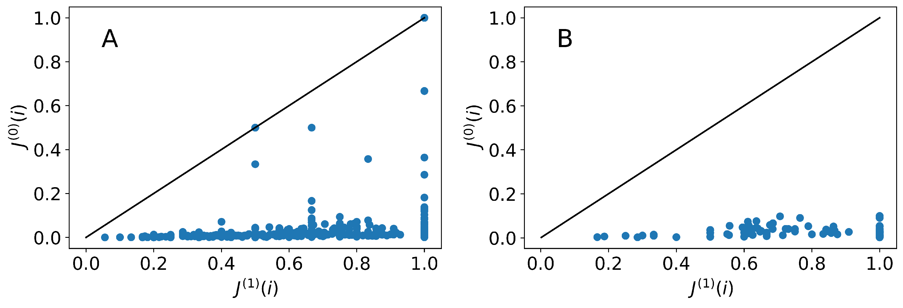
As a final check, we introduce a ratio test for careers. This check is useful for several purposes. For one, it can identify particular career sequences that are especially rare compared to random expectation. Another advantage is that it can be put to use in generating career profiles for each starting node that provide a sense for how well the collection of modeled careers match the collection of observed careers. A final use comes as an alternative to the measurements from JSD and can be readily applied to obtaining full descriptions of a model over the entire network. All these depend on the definition
which compares the observed probability of career
u with initial location
i against its simulated probability. The quantity approaches 0 as the simulated and observed probabilities of a career become more similar (i.e.,
). On the other hand, if a model overestimates the frequency of
u,
; if it is underestimated,
.
Using
over all observed careers beginning at
i provides another way to test the models. This can be done, for a given node, by measuring the average
over observed career paths, or
As indicated, this quantity can also serve as a measure of the quality of a model at the level of each individual starting point for careers. A related quantity that can be derived is the variance of
, defined as
which provides a measure of how well models capture the totality of the careers predicted to start at
i.
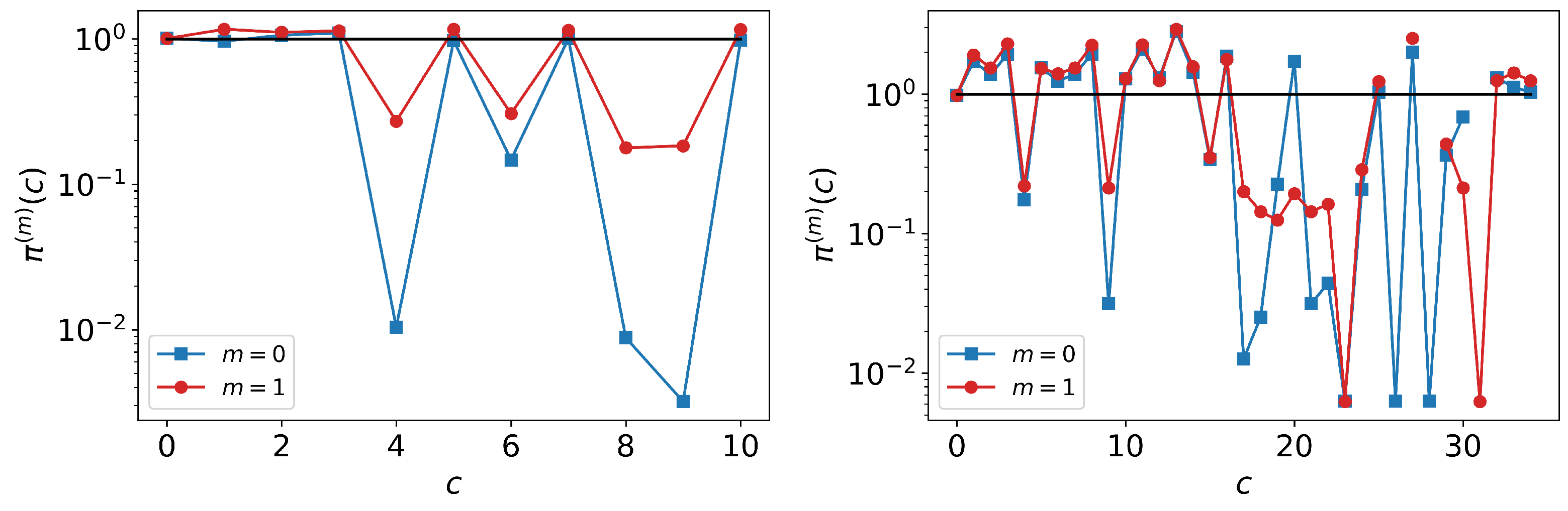
A final use for is introduce is the creation of a profile for the effectiveness of each model to recover individual observed careers. Let us create a rank-ordered list of careers so that is the most probable career departing i (that is for ). Similarly, is the second most probable career from i, which means that for . After ordering all careers, we can construct the curve where . This profile for node i shows in decreasing order of importance how closely model m is able to reproduce careers in i. A perfect model will tend to produce a flat curve of the form . On the other hand, if some careers deviate strongly, there will be noticeable jumps.


