
Hybrid Multi-Dimensional Attention U-Net for Hyperspectral Snapshot Compressive Imaging Reconstruction

1
Computer Network Information Center, Chinese Academy of Sciences, Beijing 100190, China
2
University of Chinese Academy of Sciences, Beijing 100049, China
3
School of Engineering, Westlake University, Hangzhou 310024, China
4
Shanghai Institute of Optics and Fine Mechanics, Chinese Academy of Sciences, Shanghai 201800, China
*
Author to whom correspondence should be addressed.
Entropy 2023, 25(4), 649; https://doi.org/10.3390/e25040649
Submission received: 21 March 2023
/
Revised: 10 April 2023
/
Accepted: 10 April 2023
/
Published: 12 April 2023
(This article belongs to the Special Issue Application of Information Theory to Computer Vision and Image Processing)
Abstract
:In order to capture the spatial-spectral information of the scene, various techniques have been proposed. Different from the widely used scanning-based methods, spectral snapshot compressive imaging (SCI) utilizes the idea of compressive sensing to compressively capture the 3D spatial-spectral data-cube in a single-shot 2D measurement and thus it is efficient, enjoying the advantages of high-speed and low bandwidth. However, the reconstruction process, i.e., to retrieve the 3D cube from the 2D measurement, is an ill-posed problem and it is challenging to reconstruct high quality images. Previous works usually use 2D convolutions and preliminary attention to address this challenge. However, these networks and attention do not exactly extract spectral features. On the other hand, 3D convolutions can extract more features in a 3D cube, but increase computational cost significantly. To balance this trade-off, in this paper, we propose a hybrid multi-dimensional attention U-Net (HMDAU-Net) to reconstruct hyperspectral images from the 2D measurement in an end-to-end manner. HMDAU-Net integrates 3D and 2D convolutions in an encoder–decoder structure to fully utilize the abundant spectral information of hyperspectral images with a trade-off between performance and computational cost. Furthermore, attention gates are employed to highlight salient features and suppress the noise carried by the skip connections. Our proposed HMDAU-Net achieves superior performance over previous state-of-the-art reconstruction algorithms.
1. Introduction
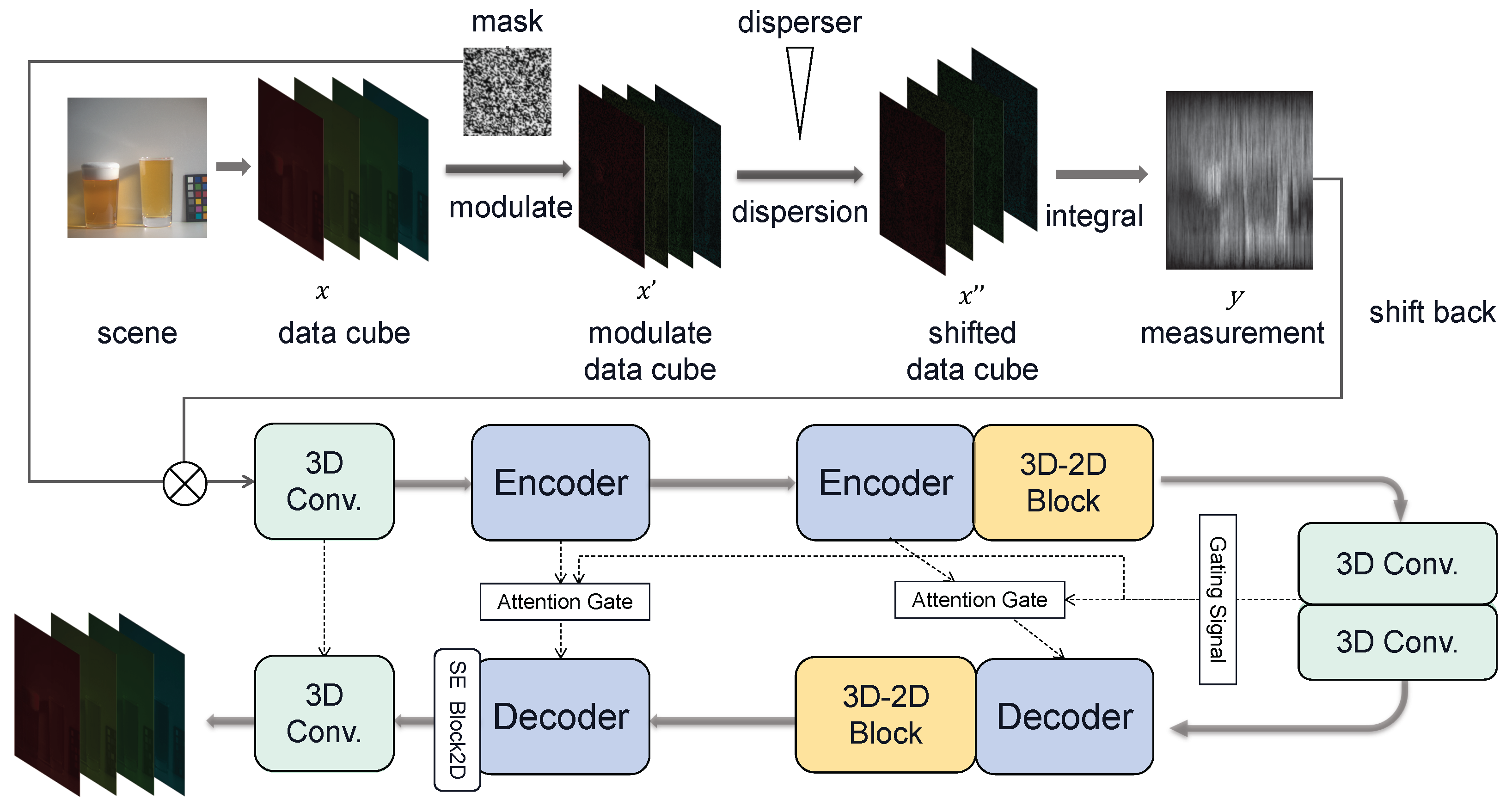
Hyperspectral images contain richer information than common RGB images and are thus widely used in various types of equipment like endoscopic system and remote sensing. To capture the rich spectral information, widely used spectrometers are mostly based on scanning to capture the three-dimensional (3D) spatial-spectral data-cube, i.e., to capture one 2D spatial frame at one wavelength in one shot and then move the next wavelength. The information captured in a 3D data-cube differs from conventional spatial coordinates [1,2], as it includes spectral information in the third dimension. Though high quality hyperspectral images can be obtained, scanning-based techniques are inefficient with respect to capturing dynamic scenes because of accuracy limitations imposed by moving objects or moving devices [3]. Thanks to compressive sensing (CS) [4,5], instead of sampling the spectral data-cube directly, the snapshot compressive-spectral imaging (SCI) [6] system samples the high dimensional data in an indirect manner. In particular, the first designed spectral SCI system, named coded aperture snapshot spectral imaging (CASSI) [7], uses a physical mask (coded aperture) and a disperser to modulate different channels (each channel corresponding to one wavelength) of the hyperspectral image and then captures the modulated data-cube in a snapshot 2D measurement by integrating across the wavelengths.
In this way, a 3D hyperspectral image can be compressed as a 2D measurement (please refer to the left part of Figure 1) and captured by an optical sensor in a short time, thus paving the way for high-speed hyperspectral image sampling [8]. With this high-speed imaging, the data storage and transmission efficiency will be extremely prompted and thus SCI has its promising prospect. After a 2D measurement is acquired, the reconstruction algorithms are employed to recover the 3D spectral data-cube (please refer to the right part of Figure 1).
It has been over 14 years since the first CASSI was built; though different variants of the hardware have been developed [11,12,13], the reconstruction algorithm has been the long-term bottleneck that precludes the wide applications of spectral SCI. Conventionally, the iterative algorithms developed for CS have been used [14,15,16,17], but have been limited by the speed [18] or performance. Fortunately, recent advances in deep learning (DL) open a new window for the inverse problem in imaging [19]. Motivated by this, different DL-based algorithms have been proposed for spectral SCI [9,20,21,22,23,24,25]. However, most existing DL methods borrow the idea from other image restoration problems; for example, both -Net [20] and TSA-Net [9] are based on U-Net [26]. These networks usually use 2D convolutional neural networks (CNNs) that ignore the strong correlation among different spectral channels in the data-cube, though some preliminary attention modules are employed. On the other hand, the 3D CNN is able to extract high-dimensional features but suffers from low speed during training and testing.
Bearing these in mind, in this paper, we propose a hybrid multi-dimensional attention U-Net (HMDAU-Net) to reconstruct hyperspectral images from the 2D measurement in an end-to-end manner. HMDAU-Net integrates 3D and 2D convolutions in an encoder–decoder structure to fully utilize the abundant spectral information of hyperspectral images with a trade-off between performance and computational cost. Furthermore, attention gates [27] are employed to highlight salient features and suppress the noise carried through the skip connections.
Note that while reconstructing hyperspectral images, we not only need to focus on the spatial resolution but also need to take the spectral resolution into consideration. Though 2D convolutions can capture spatial features well, they lack the ability to effectively investigate the spectral correlation across the third dimension. Hence, we introduce 3D CNN for reconstruction. Due to the greater computational cost of 3D CNN which will increase the inference time, we integrate 3D and 2D CNN for the trade-off of reconstruction fidelity and speed. The utilization of attention gates helps the model to suppress irrelevant regions during training which makes the model pay more attention to the reconstruction details.
1.1. Review of the CASSI System
As mentioned above, the key idea of CASSI is to modulate different wavelengths in the spectral data-cube by different weights and then integrate the light to the sensor. The first version of CASSI used a fixed mask and two dispersers to modulate the spatial information over all wavelengths in the spectral cube, termed DD-CASSI [28]; here DD means dual disperser. Following this, the single-disperser (SD) CASSI [7] was developed, which achieves modulation by removing a disperser. Below, we mathematically model the SD-CASSI sensing process.
Let denote the to-be-captured spectral data-cube at the top-left of Figure 2 and denote the fixed physical mask, where W, H and B denote the width, height and number of spectral channels, respectively. The spectral data-cube modulated by the coded aperture is , where is the same size as , and ⊙ represents the element-wise multiplication. After propagation through the disperser, each channel of is shifted along the - according to a liner dispersion and the respective wavelength. We then use , where , to denote the shifted cube and assume to be the center wavelength which is not shifted when passing through the disperser. We can obtain , where represents the coordinate system on the plane of the sensor and is the wavelength at the b-th channel; indicates the spatial shifting of the b-th channel. Thus, the 2D SCI measurement we obtain on the detector is a sum over the wavelength dimension of a mask-modulated and later shifted data-cube. It can be modeled as
where denotes the measurement noise. To facilitate the description of the model, the coding process could be considered as modulating with a shifted mask corresponding to different wavelengths and the liner dispersion d, i.e., . Correspondingly, the shifted version of the original data-cube is . According to this, the 2D measurement can be modeled as
By vectorizing the spectral data-cube and measurement, that is and , this model can be rewritten as
where denotes the sensing matrix (coded aperture) which is a concatenation of diagonal matrices, that is , where is the diagonal matrix with as the diagonal elements. Note that is a very sparse matrix and the theoretical bounds have been developed in [29,30].
After obtaining the measurement , we will focus on recovering 3D or multi-dimensional information from the 2D measurements, specifically using a novel deep learning network.
1.2. Contributions of This Work
In this paper, we propose a new end-to-end deep learning algorithm to reconstruct high quality images for the SD-CASSI system. Our contributions are summarized as follows:
- Hybrid 3D/2D CNN network: To balance the performance and computational cost, a hybrid 3D/2D block is employed to reduce parameters. Higher performance is achieved than existing 2D CNN-based algorithms; In addition, the proposed hybrid 3D/2D network shows superiority compared to the pure 3D and 2D counterparts.
- Wider rather than deeper: We evaluate that a two layer U-Net has similar performance to a four layer one in CASSI reconstructions.
- Effects of attention gate and SE (Squeeze-and-Excitation) block [33] in CASSI are evaluated. Attention gate is implemented to filter the noisy information from U-Net bottleneck and former layers. A simple 2D-CNN SE block is used to focus on important channels.
1.3. Related Work
After the first CASSI system [28] was designed, many revised CASSI were proposed. A single disperser CASSI (SD-CASSI) system was designed [7] the following year. Wang et al. [12] designed a Dual-camera CASSI system. Zhang et al. [34] proposed a novel snapshot spectral imaging system that can dynamically capture the spectral images with low computational burden and high light efficiency.
For CASSI reconstruction, the early algorithms are based on iterative optimization algorithms like TwIST [14], GAP-based [15,35] and other algorithms [16,17,18,36,37,38,39]. To promote these iterative algorithms, a deep neural network is inserted into an iteration step as a deep denoiser prior named deep plug-and-play algorithm [40]. Deep unfolding and deep unrolling methods [23,41,42,43,44,45] unfold an iterative algorithm and insert a deep learning network with better performance than common iterative algorithms and maintain their interpretation. The recent work [43] introduced a data-driven prior to exploit both the local and non-local correlations among the spectral image adaptively.
On the other hand, end-to-end deep learning-based algorithms enjoy its high reconstruction speed and excellent performance [46,47,48,49]. Researchers [22,50] proposed a CNN-based method to learn the deep prior externally (dataset) and internally (spatial-spectral constraint of inputs). Meng et al. proposed a TSA-Net [9] to exploit the self-attention mechanism to reconstruct the HSI images by capturing the information across dimensions. A generative adversarial network (GAN) [20] was also introduced in reconstruction.
Real CASSI systems always include noise and thus influence the reconstruction. Zhang et al. [51] modeled the real noise with non-zero mean that generalizes the traditional zero mean noise to characterize the optical imaging principle and boost the reconstruction quality of CASSI. The work [9] found that the shot noise is more suitable for real data training than Gaussian noise as well.
2. Proposed Network for CASSI Reconstruction
In this section, we first overview the hybrid multi-dimensional attention U-Net (HMDAU-Net). Following this, different modules of the proposed network are described in detail.
2.1. Overall Network Structure
As shown in Figure 2 (lower part), our network consists of a two layer U-Net [26] backbone, 3D–2D hybrid blocks, SE blocks and attention gates. The backbone is a two layer U-Net which is a trimmed version of TSA-Net backbone but without the attention module [9]. The encoder includes 3D CNN, 3D Res2Net and 3D maxpooling and the decoder includes 3D transpose CNN, 3D Res2Net and 3D CNN. The ReLU follows each CNN operation without batch normalization. We remove two layers from the original TSA backbone and change it into a 3D CNN with one initial 3D CNN and one end 3D CNN to match channels. A 2D SE block is employed to set the weight of the feature map and enhance the weight of important ones. Due to the large increase in parameters using cascade 3D CNN like DenseNet [52], we employ a hybrid 2D/3D CNN block named E-HCM [53] to solve our CASSI reconstruction problem. Furthermore, Attention gates [27,32] are implemented in our network to reduce inessential information among each layer.
2.2. Hybrid 2D/3D CNNs
Hyperspectral images contain abundant information across spectral channels; thus, the reconstruction needs to fully explore this information. Two-dimensional CNN extracts feature maps in each channel but lacks the content and relationship among spectral channels. To address this challenge, 3D CNN for hypterspecral image reconstruction is employed in our network. It has been observed in previous work [54] that a 3D full CNN (3D-FCNN) exploring both spatial context and spectral correlation can achieve excellent results on other applications. Different from 2D convolution, a regular 3D convolution is implemented via 3D kernels and feature maps and thus is capable of investigating correlations across spectral channels. However, 3D CNN generates a large amount of parameters during computing. Some methods use split 3D convolution to reduce parameters (i.e., splitting the filter as and ) [55] to mitigate this shortcoming. However, redundant information along the spectral dimension will be generated due to the high spatial similarity among spectral channels. This also reduces the learning ability of the model in space, which is extremely important for the reconstruction purpose as considered in our work.
To address this challenge, MCNet [56] was proposed to share the context among 3D and 2D units. A split adjacent spatial and spectral convolution (SAEC) was proposed in [53] to tackle this difficulty. It implements 3D convolution along height–width, spectral-height and spectral-width (i.e., filters are , and ). After reshaping, feature maps go through a few 2D convolution units. This hybrid 3D/2D CNN module is dubbed E-HCM. In detail, the 3D unit is employed to analyze the relationship of spectra and either horizontal or vertical direction in space. Since the spectral information is acquired, the feature maps after the 3D unit are reshaped into four dimensions to implement 2D convolution to further extract the spatial information in the desired image. Based on the consideration of efficiency and computational cost, we employ this module at the end of encoders and decoders in our HDMAU-Net.
2.3. Attention Gate
Attention Gates (AGs) [32] are initially proposed to capture a sufficiently large receptive field or semantic contextual information in medical images. The AGs are incorporated into the standard U-Net architecture to highlight salient features that are passed through the skip connections. Information extracted from the coarse scales is used in gating to disambiguate irrelevant and noisy responses in the skip connections.
As shown in Figure 2, the gating signal is generated via a 3D CNN block, including batch normalization and ReLU. The input feature in the l-th layer is . and are the sizes of a feature map (i.e., ), , and correspond to the number of feature maps. g and are inputs of the attention gate in each layer, which can be represented by:
where and denote linear transformation (e.g., , , ) conducted by 3D convolutions. , and , where and M are intermediate numbers of a feature map and sizes of a feature map, respectively. Attention coefficient . When the attention is generated, we multiply it with from skip connection and then input into decoder.
Motivated by the attention U-Net [27], the same-scale features from the encoder and decoder can be augmented and combined by attention gates. We firstly use attention gates to boost reconstruction of subtle texture in hyperspectral images and enhance the content of each layer during scale transformation in our HMDAU-Net. The output of AGs is then produced by the decoder with scaling conducted by Res2net and upsampling.
3. Experimental Results
We now verify the performance of our proposed HMDAU-Net for CASSI reconstruction, firstly on simulation data and then real data captured via the CASSI system [9]. More results are shown in Appendix A.
3.1. Simulated Data
We train our model for simulated data ( measurement on the CAVE [57], 31 spectral images of ) and test it on 10 scenes cropped from the KAIST [58] dataset provided by the TSA-Net [9], which adopts spectral interpolation on the simulation data to acquire an image of the 28 channels (ranging from 450 nm to 650 nm) as ground truth. Similar to TSA-Net, we randomly crop the hyperspectral data-cube into a spacial size of with 28 channels and then use real mask and shift the data-cube via a 2 pixel step to generate a measurement. After shifting it back to a data-cube, we put it into our network. Three-dimensional CNN need five dimensions to input and thus we unsqueeze it into a data. The number of 3D feature maps after the first 3D CNN is 32 (the second dimension). After it leaves the last block, we squeeze the data into four dimensions.
3.1.1. Comparison with State-of-the-Art Methods
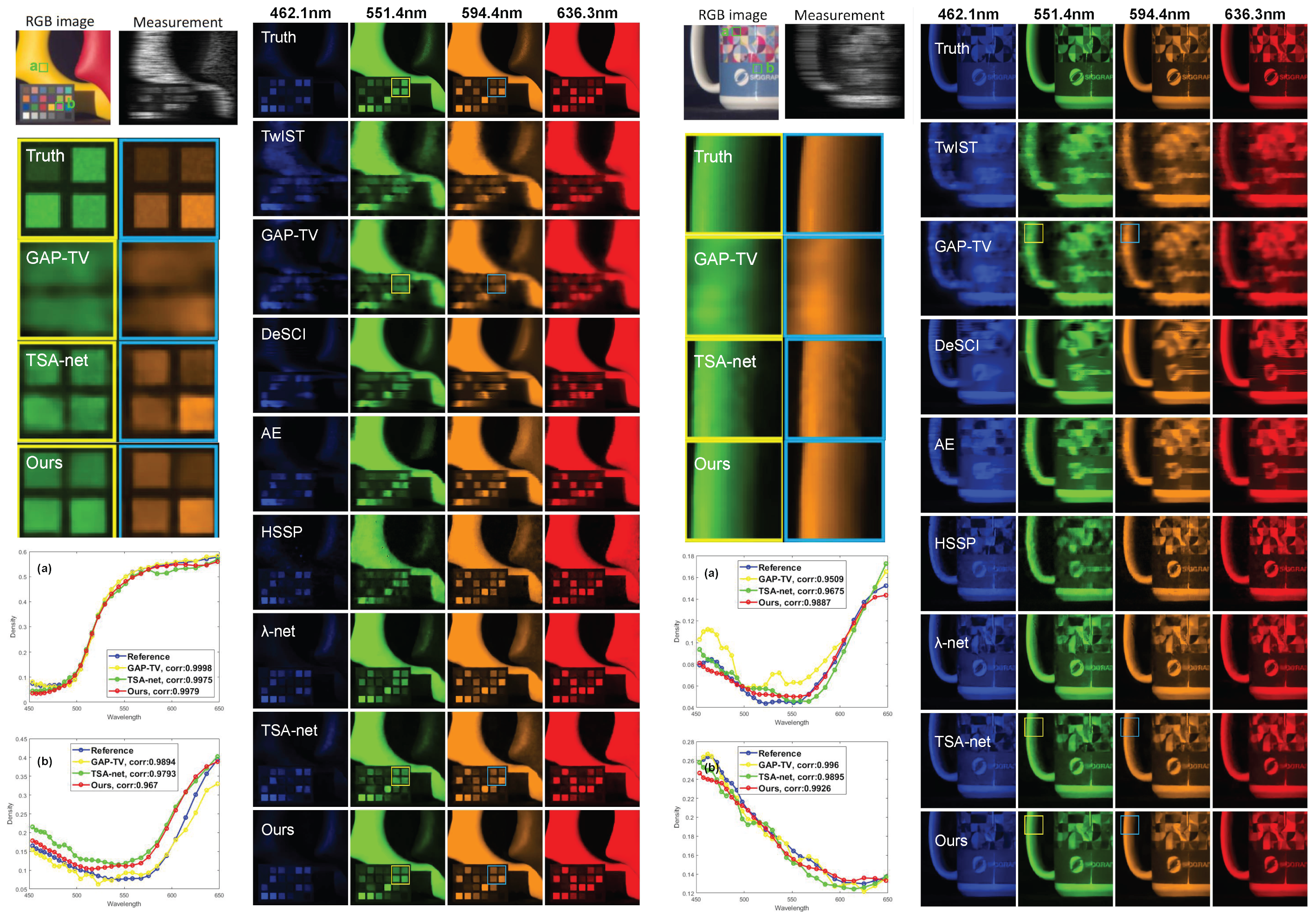
We compare our proposed reconstruction method with several state-of-the-art (SOTA) methods, including three optimization methods (TwIST [14], GAP-TV [15] and DeSCI [18]), a convolutional autoencoder-based method (AE [58]), a deep unfolding method (HSSP [23]), a GAN-based method (-Net [20]) and two end-to-end deep learning methods (U-Net [26] and TSA-Net [9]). AE does not perform as well as in the DD-CASSI system shown in Ref [58] because we use their pre-trained model which differs from our SD-CASSI data scenes, wavelenth distributions and spacial sizes. Other experimental results are from [9]. We use the same training dataset in TSA-Net and 10 scenes for test. We can see that the deep learning-based methods achieve better results and our proposed method is better than the past SOTA algorithm TSA-Net. Specifically, as shown in Table 1, our method outperforms the second best method TSA-Net by 0.6dB in average PSNR and 0.016 in average SSIM.
Figure 3 plots selected channels (4 out of 28) and spectral curves of the reconstructed images using the methods above. We can obverse that the images reconstructed via the proposed method have clearer texts and stripes. Please notice the letters on the cup and the sharp edges of the color checker. In addition, our method has more accurate spectral density than the other methods.
As depicted in Figure 3, the top-left panel showcases two designated boxes labeled “a” and “b”, accompanied by corresponding reconstructed outcomes and numerical assessments. The assessment procedure involved computing the mean values of boxes “a” and “b” across all wavelengths (each red dot represents an average value of a specific wavelength), followed by correlation analysis of the spectra based on the reference parameter. Our spectral-wise quantitative metrics are shown in the figure and clearly higher than other methods.
3.1.2. Ablation Study
We design several ablation studies to evaluate the effect of different modules in the proposed network. The comparison includes numbers of layers of U-Net backbone, attention gates and hybrid dimensional convolution modules.
To save training time, the experiments in this subsection in simulated data are trained with 16 channels when input into encoder. As shown in Table 2 left, we can observe that a two layer 3D U-Net (using the backbone in TSA-Net and replacing all convolutions by 3D-CNN) has performance similar to a four layer one in CASSI reconstruction. It even achieves 0.22 dB higher PSNR. However, by doubling the feature maps initially input into the encoder, we can see a raise of 0.44 dB. This shows that the assistance of a deeper network is not so distinct and even not beneficial to our SCI reconstruction. Instead, the wider one has much more influence. We find that this may due to the fact that too many downsamplings and upsamplings in spatial and spectral dimensions will cause information loss.
In Table 2 right, we evaluate different modules in our proposed method. Both SE block and attention gates improved our reconstruction results. In particular, SE Block can improve them more (0.25 dB in PSNR) while AGs just edge up a little bit (0.05 dB in PSNR). As we put them together, the promotion is expanded, leading to a 0.27 dB gain in PSNR. This presents the consistency of the two attentions in our reconstruction, without excessively filtering necessary spatial-spectral information.
In Table 3, we implemented different types of convolution in our U-net backbone. Our hybrid backbone uses E-HCM on the second encoder and the first decoder is a two layer U-Net backbone. E-HCM includes three 3D convolution operations and four 2D convolution operations. For the full 3D convolution, we replace the E-HCM by the same number of layer residual blocks (seven layers per module). For full 2D convolution, we replace all 3D convolution operations by 2D and keep the number of layers unchanged. For instance, taking a 2D convolution layer with kernel size K, input and output channels as an example, the number of MACs is , where and denote the height and width of the output feature map, respectively. Compared to 2D, 3D improves the PSNR value but significantly increases the computational workload as well. By using our hybrid backbone, we can decrease parameters and computational load to a large extent (40%) in contrast to 3D and even have achieved higher performance than pure 3D and 2D ones. This observation suggests that the pure 3D CNN is not as practical as 2D ones because of the soaring of computational load. However, we can mix it with 2D CNN to make a balance.
3.2. Real Data
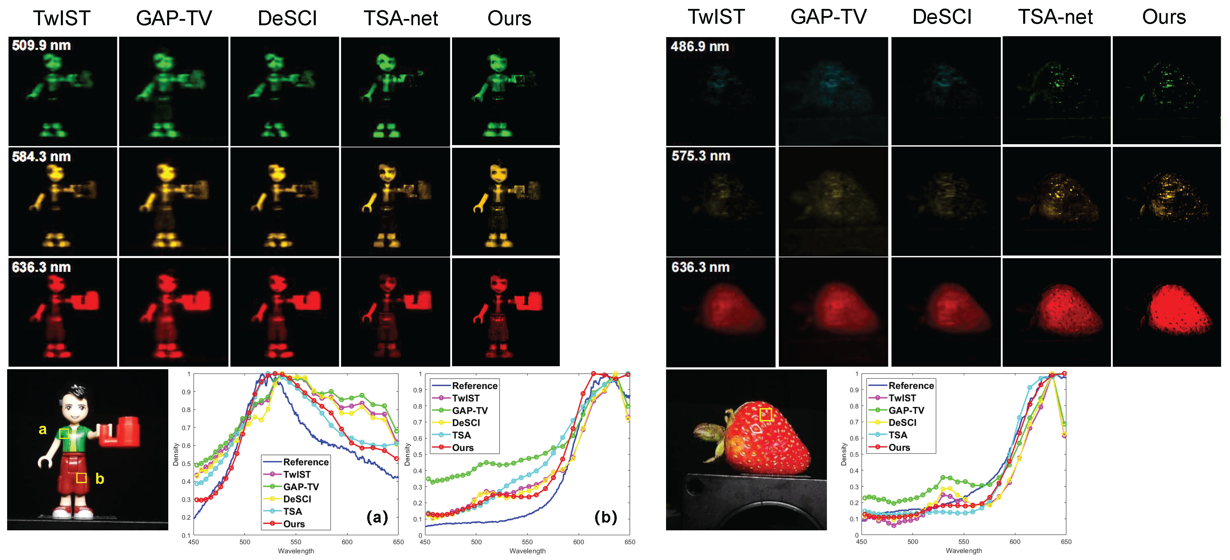
For the real data captured by the system built in [9], we again borrow the experimental results of other methods. The real data is a measurement with 28 wavelengths ranging from 450 nm to 650 nm. It was shifted 54 pixels with respect to dispersion in the column. We train our model again using the real data mask, i.e., coded mask and cropped training set. This model is much larger than the simulated one and it takes a huge increase in GPU memory usage (even more than 45 GB for batch size = 1 per batch) and time cost. Thus, we take the advantages of the Automatic Mixed Precision (AMP) module provided by Pytorch to train our model by mixed precision (half precision and single precision real numbers).
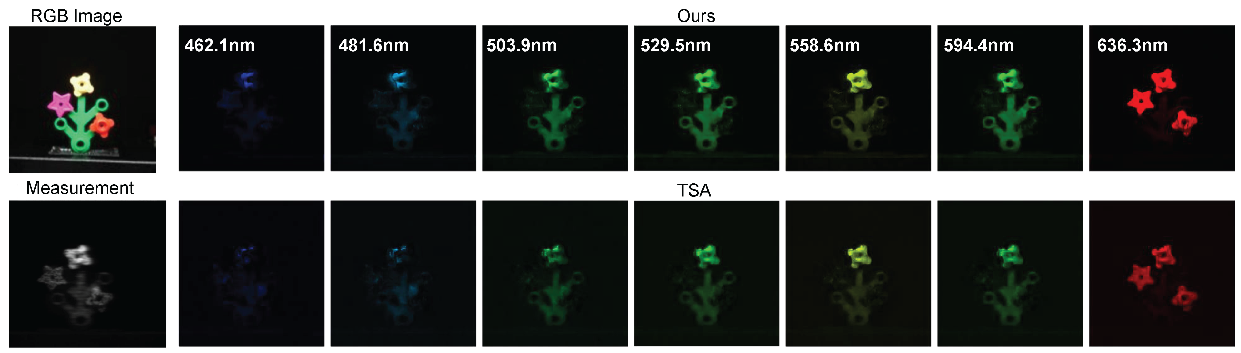
The reconstruction results of two scenes, Lego and Strawberry are shown in Figure 4, where we plot four reconstructed frames at different wavelengths and spectral density curves to demonstrate the performance of our proposed method. We observe that our result contains more detail in Legoman’s face area because our model produces sharper edges than other models. In the Strawberry testcase, our result has higher spatial resolution in all selected wavelengths. Similar to Figure 3, we attached a visualization of numerical assessment in Figure 4 and the method to obtain such assessment is the same as described above. We observe that our curve (red) is closest to the reference curve (blue) among all other curves.wo more real data results of Plants and Legoplants are shown in Figure 1 and Figure 5 with 14 and 7 selected reconstructed channels, respectively. We selected 7 spectral channels out of 28 as shown in Figure 5. Our model achieves superior reconstruction results in terms of clarity and aesthetics compared to TSA-net. Specifically, our model produces more pointed edges that elevate the overall reconstruction quality.s shown in the plots, our method provides sharper edges and more spacial details such as the hands and clothes of the Lego man. The spectral density curves reveal our method is closer to the ground truth as well.
4. Conclusions
We proposed an end-to-end hybrid multi-dimensional attention U-net for hyperspectral snapshot compressive imaging reconstruction. The algorithm employed hybrid 3D/2D convolutions instead of using one of them alone to balance the trade-off of computational cost and performance. Our proposed network achieved superior results over previous end-to-end CNN based algorithms.
One important observation from our experiments is that for SCI reconstruction tasks, it is not necessary that the backbone network (e.g., U-Net) be deep, but it needs to be wider (more kernels in each layer) to provide good results. This may due to the task difference between image reconstruction (to recover details) and image classification (to extract features). We further used the attention gate to extract essential correlations in the spectral data-cube to improve the reconstruction performance in our network.
Author Contributions
Conceptualization, S.Z. and M.C.; Methodology, S.Z. and M.Z.; Software, S.Z.; Validation, S.Z.; Writing—original draft, S.Z.; Writing—review & editing, M.Z. and M.C. All authors have read and agreed to the published version of the manuscript.
Funding
This work was supported by the National Natural Science Foundation of China under Grant No. 62271414, Zhejiang Provincial Natural Science Foundation of China under Grant No. LR23F010001. We would like to thank Research Center for Industries of the Future (RCIF) at Westlake University for supporting this work and the funding from Lochn Optics.
Institutional Review Board Statement
Not applicable.
Data Availability Statement
The data that support the plots within these paper and other findings of this study are available from the corresponding authors upon reasonable request.
Conflicts of Interest
The authors declare no conflict of interest.
Appendix A. Experimental Results
Appendix A.1. Simulated Data Results
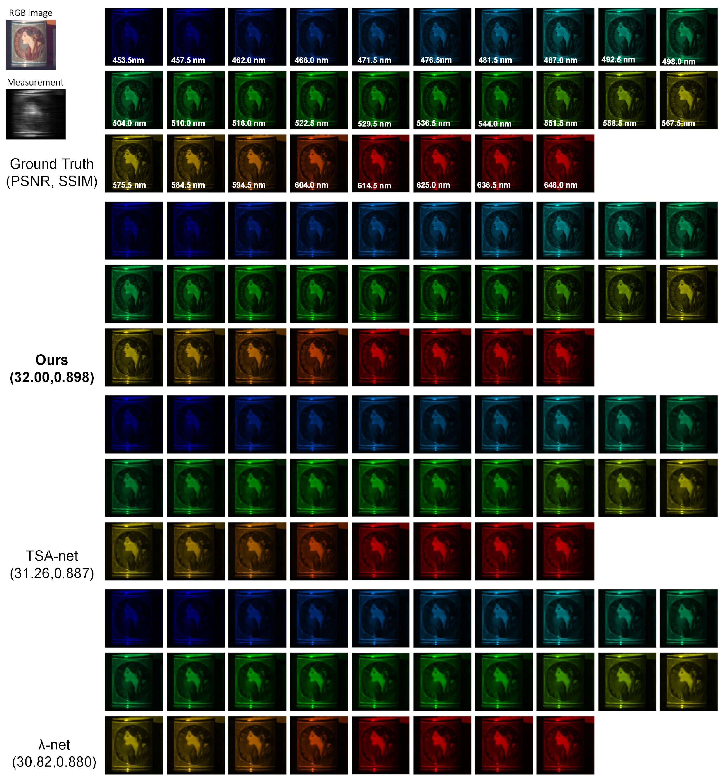
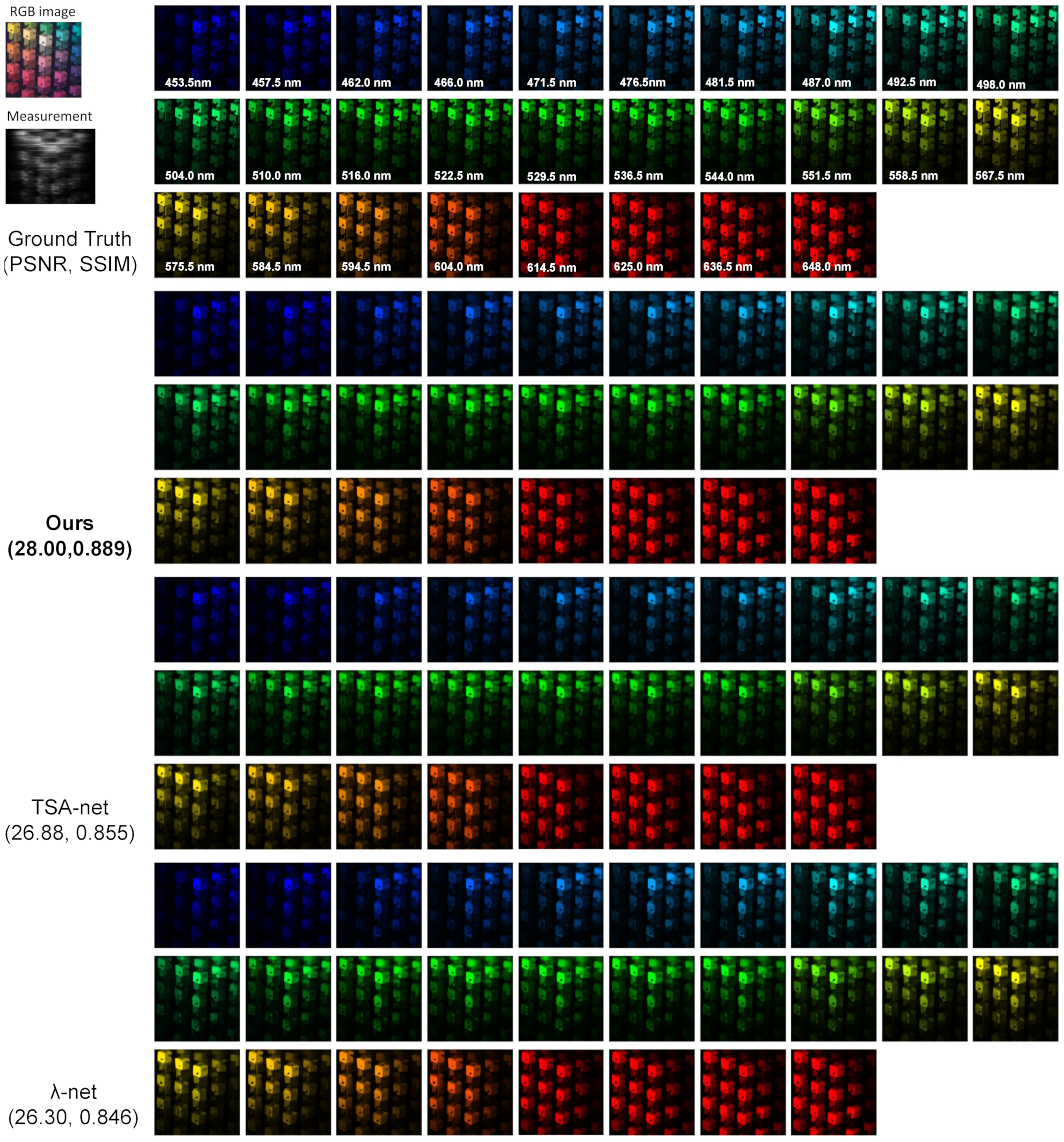
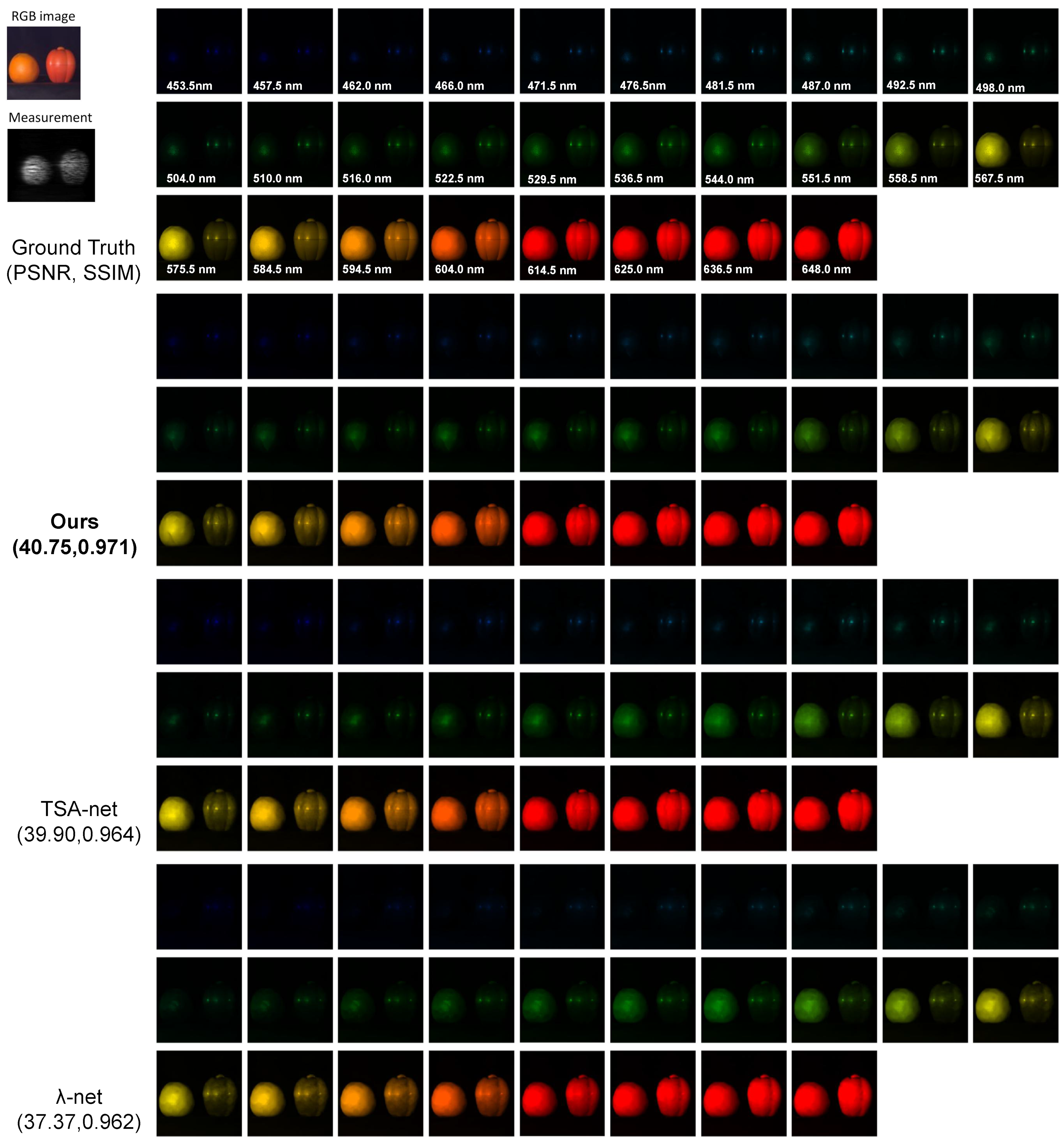
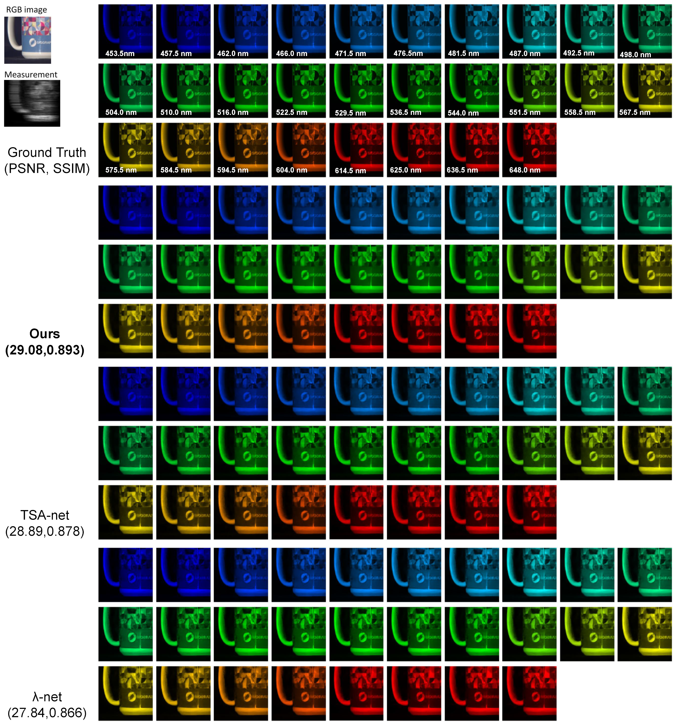
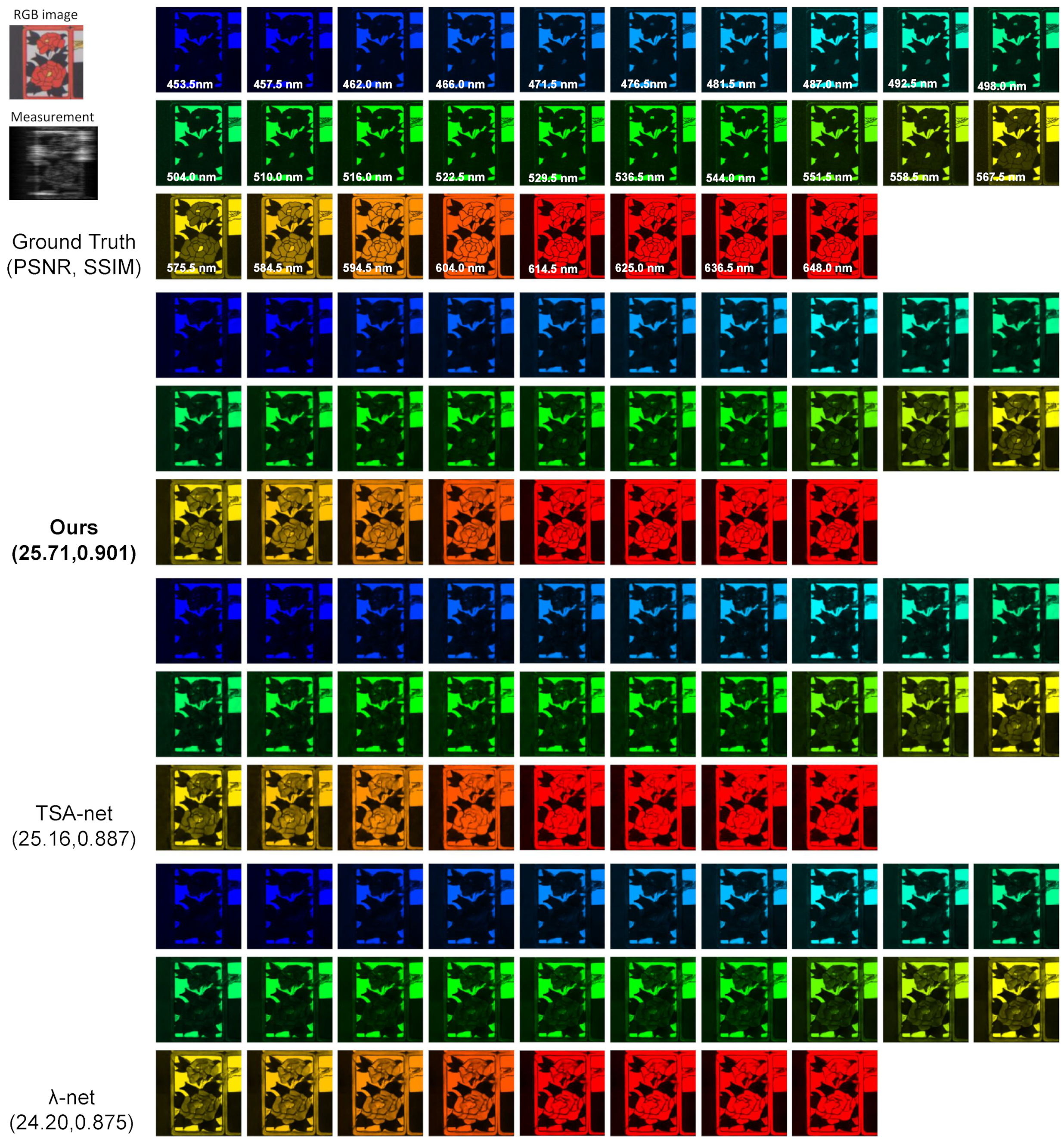
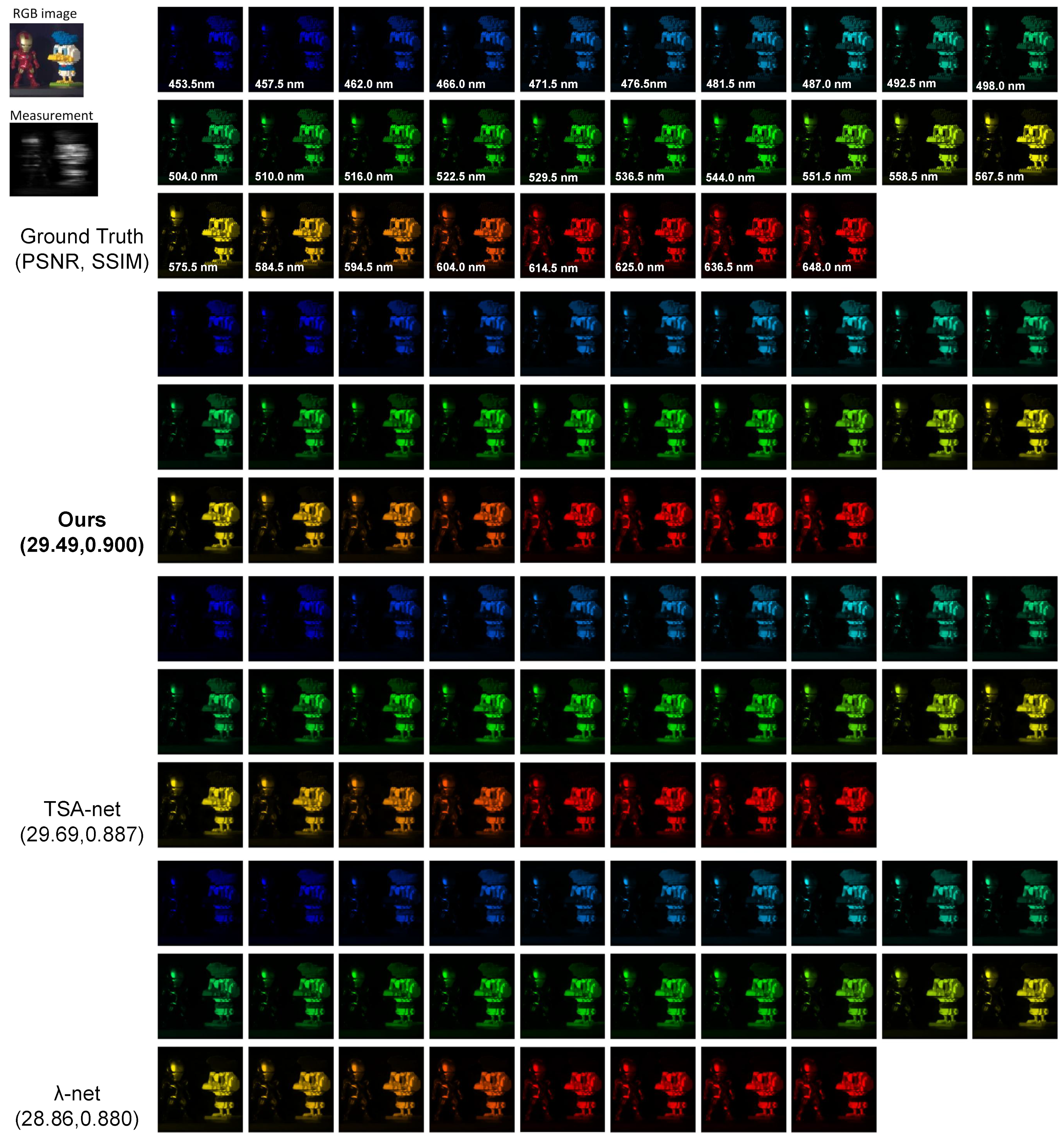
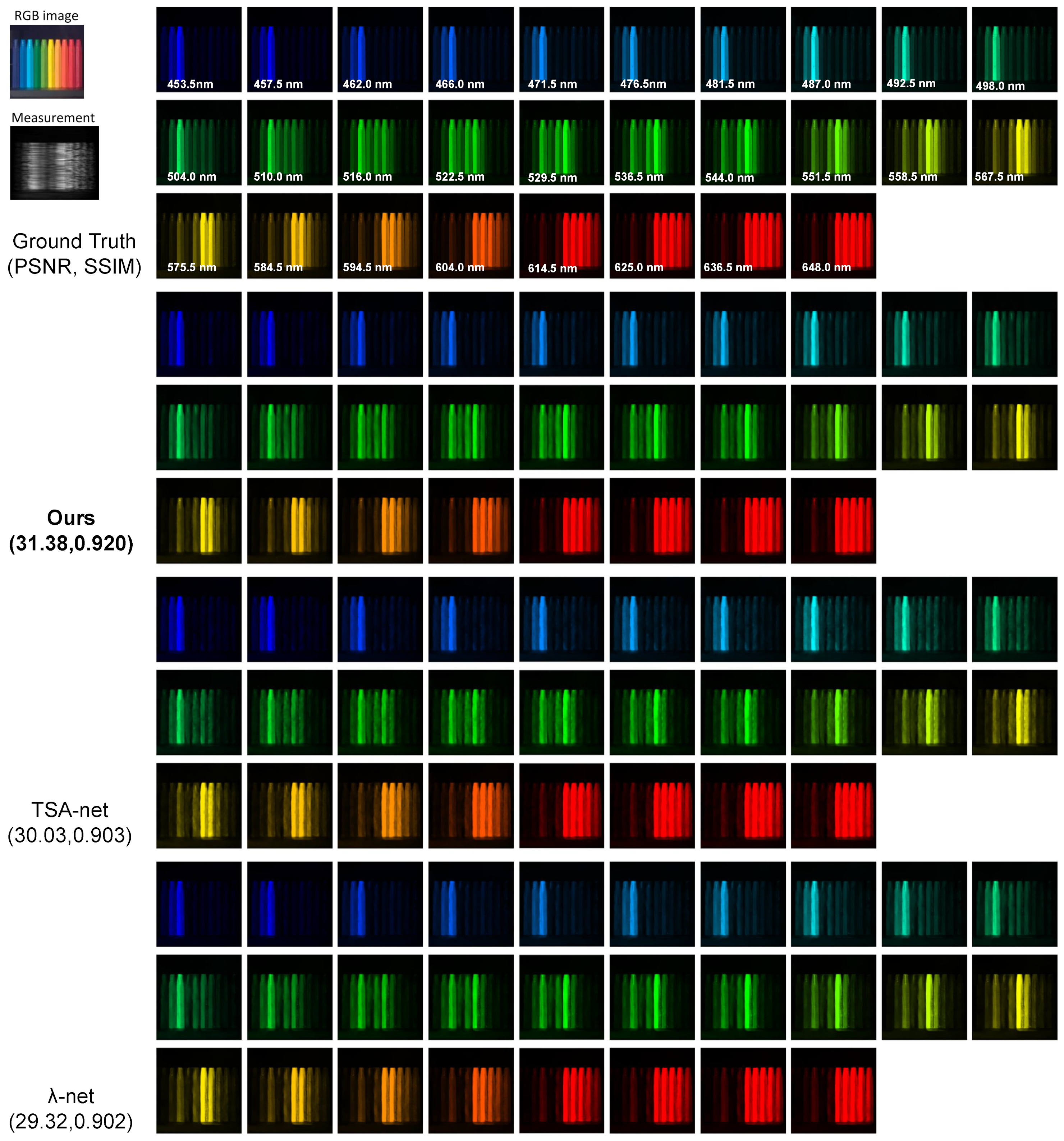
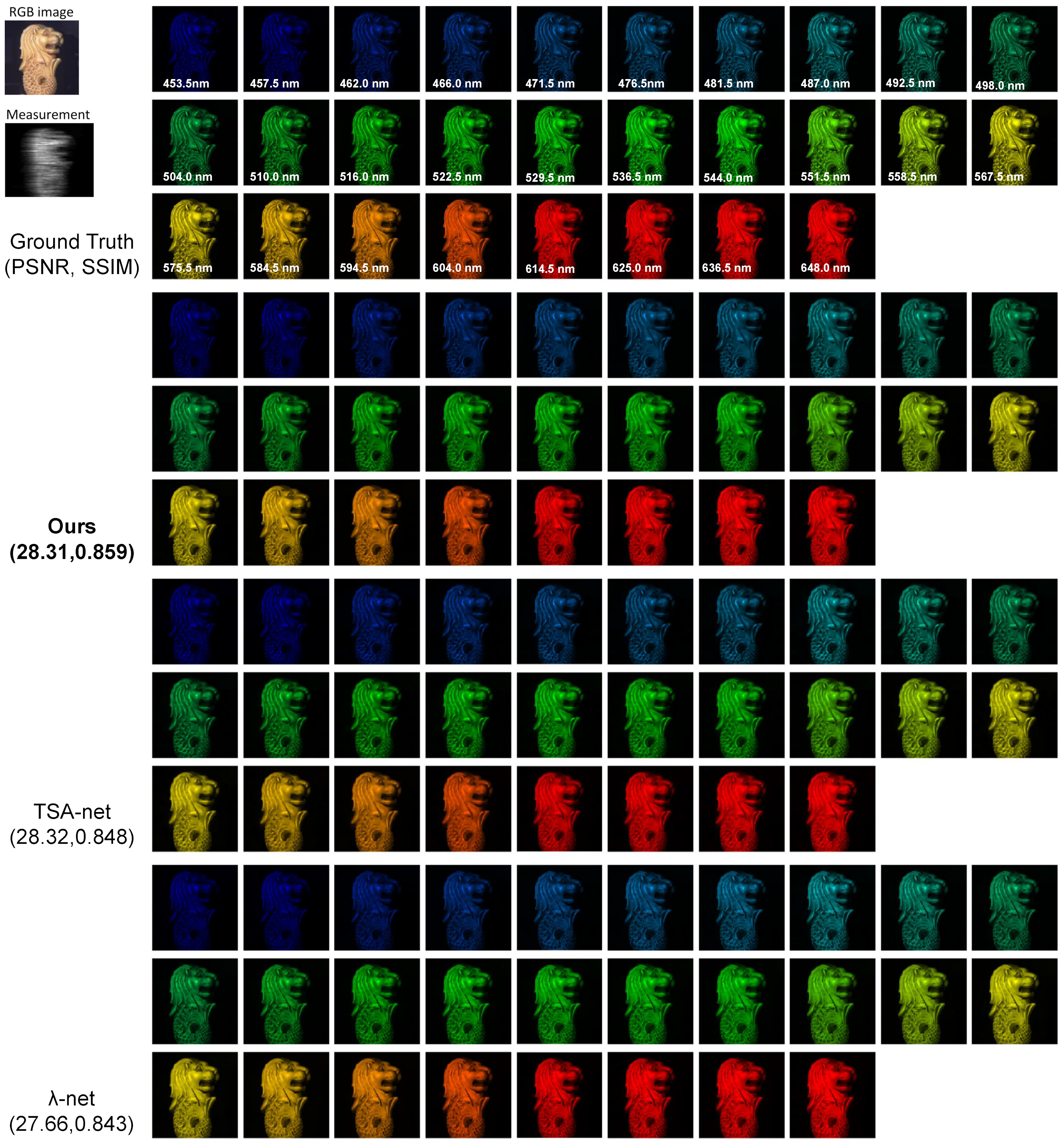
Figure A1, Figure A2, Figure A3, Figure A4, Figure A5, Figure A6, Figure A7, Figure A8, Figure A9 and Figure A10 show the simulation results with 28 spectral channels for 10 scenes from KAIST. Truth, measurements and RGB images are shown for reference. We compare our proposed method with the TSA-net and -net algorithms and list the corresponding PSNR and SSIM.
Figure A1.
Simulation: RGB image, measurement, ground truth and reconstructed results by Tour proposed method with the TSA-net and -net Scene 1. The PSNR in dB and SSIM for the result images are shown in the parenthesis.
Figure A1.
Simulation: RGB image, measurement, ground truth and reconstructed results by Tour proposed method with the TSA-net and -net Scene 1. The PSNR in dB and SSIM for the result images are shown in the parenthesis.

Figure A2.
Simulation: RGB image, measurement, ground truth and reconstructed results by Tour proposed method with the TSA-net and -net Scene 2. The PSNR in dB and SSIM for the result images are shown in the parenthesis.
Figure A2.
Simulation: RGB image, measurement, ground truth and reconstructed results by Tour proposed method with the TSA-net and -net Scene 2. The PSNR in dB and SSIM for the result images are shown in the parenthesis.

Figure A3.
Simulation: RGB image, measurement, ground truth and reconstructed results by Tour proposed method with the TSA-net and -net Scene 3. The PSNR in dB and SSIM for the result images are shown in the parenthesis.
Figure A3.
Simulation: RGB image, measurement, ground truth and reconstructed results by Tour proposed method with the TSA-net and -net Scene 3. The PSNR in dB and SSIM for the result images are shown in the parenthesis.

Figure A4.
Simulation: RGB image, measurement, ground truth and reconstructed results by Tour proposed method with the TSA-net and -net Scene 4. The PSNR in dB and SSIM for the result images are shown in the parenthesis.
Figure A4.
Simulation: RGB image, measurement, ground truth and reconstructed results by Tour proposed method with the TSA-net and -net Scene 4. The PSNR in dB and SSIM for the result images are shown in the parenthesis.

Figure A5.
Simulation: RGB image, measurement, ground truth and reconstructed results by Tour proposed method with the TSA-net and -net Scene 5. The PSNR in dB and SSIM for the result images are shown in the parenthesis.
Figure A5.
Simulation: RGB image, measurement, ground truth and reconstructed results by Tour proposed method with the TSA-net and -net Scene 5. The PSNR in dB and SSIM for the result images are shown in the parenthesis.

Figure A6.
Simulation: RGB image, measurement, ground truth and reconstructed results by Tour proposed method with the TSA-net and -net Scene 6. The PSNR in dB and SSIM for the result images are shown in the parenthesis.
Figure A6.
Simulation: RGB image, measurement, ground truth and reconstructed results by Tour proposed method with the TSA-net and -net Scene 6. The PSNR in dB and SSIM for the result images are shown in the parenthesis.

Figure A7.
Simulation: RGB image, measurement, ground truth and reconstructed results by Tour proposed method with the TSA-net and -net Scene 7. The PSNR in dB and SSIM for the result images are shown in the parenthesis.
Figure A7.
Simulation: RGB image, measurement, ground truth and reconstructed results by Tour proposed method with the TSA-net and -net Scene 7. The PSNR in dB and SSIM for the result images are shown in the parenthesis.

Figure A8.
Simulation: RGB image, measurement, ground truth and reconstructed results by Tour proposed method with the TSA-net and -net Scene 8. The PSNR in dB and SSIM for the result images are shown in the parenthesis.
Figure A8.
Simulation: RGB image, measurement, ground truth and reconstructed results by Tour proposed method with the TSA-net and -net Scene 8. The PSNR in dB and SSIM for the result images are shown in the parenthesis.

Figure A9.
Simulation: RGB image, measurement, ground truth and reconstructed results by Tour proposed method with the TSA-net and -net Scene 9. The PSNR in dB and SSIM for the result images are shown in the parenthesis.
Figure A9.
Simulation: RGB image, measurement, ground truth and reconstructed results by Tour proposed method with the TSA-net and -net Scene 9. The PSNR in dB and SSIM for the result images are shown in the parenthesis.

Figure A10.
Simulation: RGB image, measurement, ground truth and reconstructed results by Tour proposed method with the TSA-net and -net Scene 10. The PSNR in dB and SSIM for the result images are shown in the parenthesis.
Figure A10.
Simulation: RGB image, measurement, ground truth and reconstructed results by Tour proposed method with the TSA-net and -net Scene 10. The PSNR in dB and SSIM for the result images are shown in the parenthesis.

Appendix A.2. Real Data Results
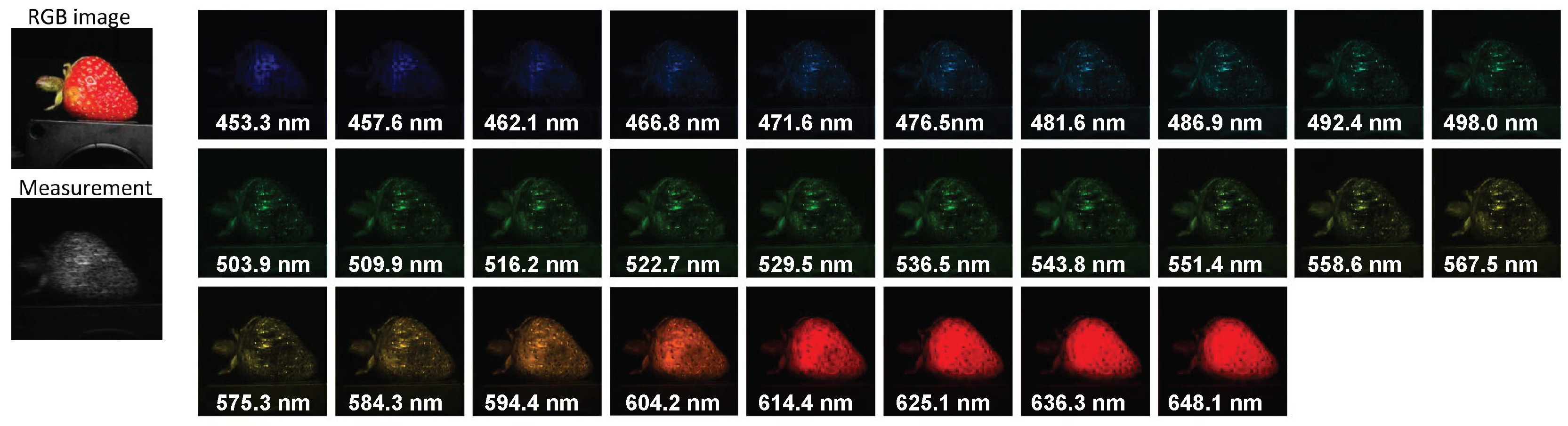
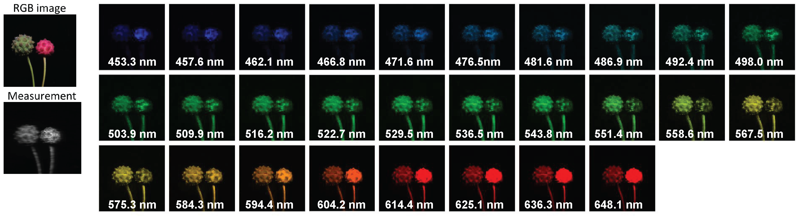
Figure A11, Figure A12, Figure A13 and Figure A14 show the RGB images, measurements and the reconstructed 28 spectral channels for four real scenes with a size of 660 × 660 pixels captured by real CASSI system.
Figure A11.
Real data: RGB image, measurement and reconstructed results by our proposed method for scene 1.
Figure A11.
Real data: RGB image, measurement and reconstructed results by our proposed method for scene 1.

Figure A12.
Real data: RGB image, measurement and reconstructed results by our proposed method for scene 2.
Figure A12.
Real data: RGB image, measurement and reconstructed results by our proposed method for scene 2.

Figure A13.
Real data: RGB image, measurement and reconstructed results by our proposed method for scene 3.
Figure A13.
Real data: RGB image, measurement and reconstructed results by our proposed method for scene 3.

Figure A14.
Real data: RGB image, measurement and reconstructed results by our proposed method for scene 4.
Figure A14.
Real data: RGB image, measurement and reconstructed results by our proposed method for scene 4.

References
- Flores-Fuentes, W.; Trujillo-Hernández, G.; Alba-Corpus, I.Y.; Rodríguez-Quiñonez, J.C.; Mirada-Vega, J.E.; Hernández-Balbuena, D.; Murrieta-Rico, F.N.; Sergiyenko, O. 3D spatial measurement for model reconstruction: A review. Measurement 2023, 207, 112321. [Google Scholar] [CrossRef]
- Rodríguez-Quiñonez, J.C.; Sergiyenko, O.; Flores-Fuentes, W.; Lopez, M.; Hernez-Balbuena, D.; Rascon, R.; Mercorelli, P. Improve a 3D distance measurement accuracy in stereo vision systems using optimization methods’ approach. Opto-Electron. Rev. 2017, 25, 24–32. [Google Scholar] [CrossRef]
- Rodríguez-Quiñonez, J.C.; Sergiyenko, O.; Hernandez-Balbuena, D.; Rivas-Lopez, M.; Flores-Fuentes, W.; Basaca-Preciado, L.C. Improve 3D laser scanner measurements accuracy using a FFBP neural network with Widrow-Hoff weight/bias learning function. Opto-Electron 2014, 22, 224–235. [Google Scholar] [CrossRef]
- Emannuel, C.; Romberg, J.; Tao, T. Robust uncertainty principles: Exact signal reconstruction from highly incomplete frequency information. IEEE Trans. Inf. Theory 2006, 52, 489–509. [Google Scholar]
- Donoho, D.L. Compressed sensing. IEEE Trans. Inf. Theory 2006, 52, 1289–1306. [Google Scholar] [CrossRef]
- Yuan, X.; Brady, D.J.; Katsaggelos, A.K. Snapshot Compressive Imaging: Theory, Algorithms and Applications. IEEE Signal Process. Mag. 2021, 38, 65–88. [Google Scholar] [CrossRef]
- Wagadarikar, A.; John, R.; Willett, R.; Brady, D. Single disperser design for coded aperture snapshot spectral imaging. Appl. Opt. 2008, 47, B44–B51. [Google Scholar] [CrossRef] [Green Version]
- Tsai, T.H.; Llull, P.; Yuan, X.; Carin, L.; Brady, D.J. Spectral-temporal compressive imaging. Opt. Lett. 2015, 40, 4054–4057. [Google Scholar] [CrossRef]
- Meng, Z.; Ma, J.; Yuan, X. End-to-End Low Cost Compressive Spectral Imaging with Spatial-Spectral Self-Attention. In Proceedings of the European Conference on Computer Vision (ECCV), Glasgow, UK, 23–28 August 2020. [Google Scholar]
- Wang, Z.; Bovik, A.C.; Sheikh, H.R.; Simoncelli, E.P. Image quality assessment: From error visibility to structural similarity. IEEE Trans. Image Process. 2004, 13, 600–612. [Google Scholar] [CrossRef] [Green Version]
- Yuan, X.; Tsai, T.H.; Zhu, R.; Llull, P.; Brady, D.; Carin, L. Compressive Hyperspectral Imaging with Side Information. IEEE J. Sel. Top. Signal Process. 2015, 9, 964–976. [Google Scholar] [CrossRef] [Green Version]
- Wang, L.; Xiong, Z.; Gao, D.; Shi, G.; Wu, F. Dual-camera design for coded aperture snapshot spectral imaging. Appl. Opt. 2015, 54, 848–858. [Google Scholar] [CrossRef] [PubMed] [Green Version]
- Arguello, H.; Rueda, H.; Wu, Y.; Prather, D.W.; Arce, G.R. Higher-order computational model for coded aperture spectral imaging. Appl. Opt. 2013, 52, D12–D21. [Google Scholar] [CrossRef] [PubMed]
- Bioucas-Dias, J.; Figueiredo, M. A New TwIST: Two-Step Iterative Shrinkage/Thresholding Algorithms for Image Restoration. IEEE Trans. Image Process. 2007, 16, 2992–3004. [Google Scholar] [CrossRef] [Green Version]
- Yuan, X. Generalized alternating projection based total variation minimization for compressive sensing. In Proceedings of the 2016 IEEE International Conference on Image Processing (ICIP), Pheonix, AZ, USA, 25–28 September 2016. [Google Scholar]
- Yang, J.; Liao, X.; Yuan, X.; Llull, P.; Brady, D.J.; Sapiro, G.; Carin, L. Compressive Sensing by Learning a Gaussian Mixture Model from Measurements. IEEE Trans. Image Process. 2015, 24, 106–119. [Google Scholar] [CrossRef] [PubMed]
- Wang, L.; Xiong, Z.; Shi, G.; Wu, F.; Zeng, W. Adaptive Nonlocal Sparse Representation for Dual-Camera Compressive Hyperspectral Imaging. IEEE Trans. Pattern Anal. Mach. Intell. 2017, 39, 2104–2111. [Google Scholar] [CrossRef]
- Liu, Y.; Yuan, X.; Suo, J.; Brady, D.J.; Dai, Q. Rank Minimization for Snapshot Compressive Imaging. IEEE Trans. Pattern Anal. Mach. Intell. 2019, 41, 2990–3006. [Google Scholar] [CrossRef] [Green Version]
- Ongie, G.; Jalal, A.; Metzler, C.A.; Baraniuk, R.G.; Dimakis, A.G.; Willett, R. Deep Learning Techniques for Inverse Problems in Imaging. IEEE J. Sel. Areas Inf. Theory 2020, 1, 39–56. [Google Scholar] [CrossRef]
- Miao, X.; Yuan, X.; Pu, Y.; Athitsos, V. λ-net: Reconstruct Hyperspectral Images from a Snapshot Measurement. In Proceedings of the IEEE/CVF Conference on Computer Vision (ICCV), Seoul, Republic of Korea, 27 October–2 November 2019. [Google Scholar]
- Meng, Z.; Jalali, S.; Yuan, X. GAP-net for Snapshot Compressive Imaging. arXiv 2020, arXiv:2012.08364. [Google Scholar]
- Fu, Y.; Zhang, T.; Wang, L.; Huang, H. Coded Hyperspectral Image Reconstruction using Deep External and Internal Learning. IEEE Trans. Pattern Anal. Mach. Intell. 2021, 44, 3404–3420. [Google Scholar] [CrossRef]
- Wang, L.; Sun, C.; Fu, Y.; Kim, M.H.; Huang, H. Hyperspectral Image Reconstruction Using a Deep Spatial-Spectral Prior. In Proceedings of the 2019 IEEE/CVF Conference on Computer Vision and Pattern Recognition (CVPR), Long Beach, CA, USA, 16–20 June 2019. [Google Scholar]
- Yu, Z.; Liu, D.; Cheng, L.; Meng, Z.; Zhao, Z.; Yuan, X.; Xu, K. Deep learning enabled reflective coded aperture snapshot spectral imaging. Opt. Express 2022, 30, 46822–46837. [Google Scholar] [CrossRef]
- Wang, Y.; Han, Y.; Wang, K.; Zhao, X. Total variation regularized nonlocal low-rank tensor train for spectral compressive imaging. Singal Process. 2022, 195, 108464. [Google Scholar] [CrossRef]
- Ronneberger, O.; Fischer, P.; Brox, T. U-Net: Convolutional Networks for Biomedical Image Segmentation. In Proceedings of the International Conference on Medical Image Computing and Computer-Assisted Intervention (MICCAI), Munich, Germany, 5–9 October 2015. [Google Scholar]
- Oktay, O.; Schlemper, J.; Folgoc, L.L.; Lee, M.; Heinrich, M.P.; Misawa, K.; Mori, K.; McDonagh, S.; Hammerla, N.Y.; Kainz, B.; et al. Attention U-Net: Learning Where to Look for the Pancreas. Med. Image Anal. 2018, 51, 63–76. [Google Scholar]
- Gehm, M.E.; John, R.; Brady, D.J.; Willett, R.M.; Schulz, T.J. Single-shot compressive spectral imaging with a dual-disperser architecture. Opt. Express 2007, 15, 14013–14027. [Google Scholar] [CrossRef] [PubMed] [Green Version]
- Jalali, S.; Yuan, X. Compressive imaging via one-shot measurements. In Proceedings of the 2018 IEEE International Symposium on Information Theory (ISIT), Vail, CO, USA, 17–23 June 2018. [Google Scholar]
- Jalali, S.; Yuan, X. Snapshot compressed sensing: Performance bounds and algorithms. IEEE Trans. Inf. Theory 2019, 65, 8005–8024. [Google Scholar] [CrossRef] [Green Version]
- Gao, S.H.; Cheng, M.M.; Zhao, K.; Zhang, X.Y.; Yang, M.H.; Torr, P.H. Res2net: A new multi-scale backbone architecture. IEEE Trans. Pattern Anal. Mach. Intell. 2019, 43, 652–662. [Google Scholar] [CrossRef] [Green Version]
- Schlemper, J.; Oktay, O.; Chen, L.; Matthew, J.; Knight, C.; Kainz, B.; Glocker, B.; Rueckert, D. Attention-Gated Networks for Improving Ultrasound Scan Plane Detection. IEEE Trans. Med. Imaging 2018, 38, 5, 1069–1078. [Google Scholar]
- Hu, J.; Shen, L.; Sun, G. Squeeze-and-excitation networks. In Proceedings of the IEEE Conference on Computer Vision and Pattern Recognition (CVPR), Salt Lake City, UT, USA, 19–21 June 2018. [Google Scholar]
- Zhang, M.; Wang, L.; Zhang, L.; Huang, H. High light efficiency snapshot spectral imaging via spatial multiplexing and spectral mixing. Opt. Express 2020, 28, 19837–19850. [Google Scholar] [CrossRef]
- Liao, X.; Li, H.; Carin, L. Generalized Alternating Projection for Weighted-ℓ2,1 Minimization with Applications to Model-based Compressive Sensing. SIAM J. Imaging Sci. 2014, 7, 797–823. [Google Scholar] [CrossRef]
- Zhang, S.; Wang, L.; Fu, Y.; Zhong, X.; Huang, H. Computational hyperspectral imaging based on dimension-discriminative low-rank tensor recovery. In Proceedings of the IEEE/CVF International Conference on Computer Vision (ICCV), Seoul, Republic of Korea, 27 October–2 November 2019. [Google Scholar]
- Golbabaee, M.; Vandergheynst, P. Hyperspectral image compressed sensing via low-rank and joint-sparse matrix recovery. In Proceedings of the 2012 IEEE International Conference on Acoustics, Speech and Signal Processing (ICASSP), Kyoto, Japan, 25–30 March 2012. [Google Scholar]
- Gelvez, T.; Rueda, H.; Arguello, H. Joint sparse and low rank recovery algorithm for compressive hyperspectral imaging. Appl. Opt. 2017, 56, 6785–6795. [Google Scholar] [CrossRef]
- Fu, Y.; Zheng, Y.; Sato, I.; Sato, Y. Exploiting spectral-spatial correlation for coded hyperspectral image restoration. In Proceedings of the IEEE Conference on Computer Vision and Pattern Recognition (CVPR), Las Vegas, NV, USA, 26 June–1 July 2016. [Google Scholar]
- Zheng, S.; Liu, Y.; Meng, Z.; Qiao, M.; Tong, Z.; Yang, X.; Han, S.; Yuan, X. Deep plug-and-play priors for spectral snapshot compressive imaging. Photonics Res. 2021, 9, B18–B29. [Google Scholar] [CrossRef]
- Yang, Y.; Sun, J.; Li, H.; Xu, Z. Deep ADMM-Net for Compressive Sensing MRI. In Proceedings of the Neural Information Processing Systems 29, Barcelona, Spain, 5–10 December 2016. [Google Scholar]
- Ma, J.; Liu, X.; Shou, Z.; Yuan, X. Deep Tensor ADMM-Net for Snapshot Compressive Imaging. In Proceedings of the IEEE/CVF Conference on Computer Vision (ICCV), Seoul, Republic of Korea, 27 October–2 November 2019. [Google Scholar]
- Wang, L.; Sun, C.; Zhang, M.; Fu, Y.; Huang, H. DNU: Deep Non-Local Unrolling for Computational Spectral Imaging. In Proceedings of the IEEE/CVF Conference on Computer Vision and Pattern Recognition (CVPR), Virtual, 14–19 June 2020. [Google Scholar]
- Zhang, J.; Ghanem, B. ISTA-Net: Interpretable optimization-inspired deep network for image compressive sensing. In Proceedings of the IEEE Conference on Computer Vision and Pattern Recognition (CVPR), Salt Lake City, UT, USA, 19–21 June 2018. [Google Scholar]
- Sogabe, Y.; Sugimoto, S.; Kurozumi, T.; Kimata, H. ADMM-Inspired Reconstruction Network for Compressive Spectral Imaging. In Proceedings of the 2020 IEEE International Conference on Image Processing (ICIP), Abu Dhabi, United Arab Emirates, 25–28 October 2020. [Google Scholar]
- Li, H.; Xiong, Z.; Shi, Z.; Wang, L.; Liu, D.; Wu, F. HSVCNN: CNN-based hyperspectral reconstruction from RGB videos. In Proceedings of the 2018 IEEE International Conference on Image Processing (ICIP), Athens, Greece, 7–10 October 2018. [Google Scholar]
- Xiong, Z.; Shi, Z.; Li, H.; Wang, L.; Liu, D.; Wu, F. Hscnn: Cnn-based hyperspectral image recovery from spectrally undersampled projections. In Proceedings of the IEEE International Conference on Computer Vision Workshops, Venice, Italy, 22–29 October 2017. [Google Scholar]
- Wang, L.; Zhang, T.; Fu, Y.; Huang, H. Hyperreconnet: Joint coded aperture optimization and image reconstruction for compressive hyperspectral imaging. IEEE Trans. Image Process. 2018, 28, 2257–2270. [Google Scholar] [CrossRef] [PubMed]
- Kohei, Y.; Han, X.H. Deep Residual Attention Network for Hyperspectral Image Reconstruction. In Proceedings of the 2020 25th International Conference on Pattern Recognition (ICPR), Milan, Italy, 10–15 January 2021. [Google Scholar]
- Zhang, T.; Fu, Y.; Wang, L.; Huang, H. Hyperspectral image reconstruction using deep external and internal learning. In Proceedings of the IEEE/CVF International Conference on Computer Vision (ICCV), Seoul, Republic of Korea, 27 October–2 November 2019. [Google Scholar]
- Zhang, M.; Wang, L.; Zhang, L.; Huang, H. Compressive hyperspectral imaging with non-zero mean noise. Opt. Express 2019, 27, 17449–17462. [Google Scholar] [CrossRef] [PubMed]
- Huang, G.; Liu, Z.; Van Der Maaten, L.; Weinberger, K.Q. Densely connected convolutional networks. In Proceedings of the IEEE Conference on Computer Vision and Pattern Recognition (CVPR), Honolulu, HI, USA, 21–26 July 2017. [Google Scholar]
- Li, Q.; Wang, Q.; Li, X. Exploring the Relationship Between 2D/3D Convolution for Hyperspectral Image Super-Resolution. IEEE Trans. Geosci. Remote Sens. 2021, 59, 5622–5637. [Google Scholar] [CrossRef]
- Mei, S.; Yuan, X.; Ji, J.; Zhang, Y.; Wan, S.; Du, Q. Hyperspectral image spatial super-resolution via 3D full convolutional neural network. Remote Sens. 2017, 9, 1139. [Google Scholar] [CrossRef] [Green Version]
- Wang, Q.; Li, Q.; Li, X. Spatial-Spectral Residual Network for Hyperspectral Image Super-Resolution. arXiv 2020, arXiv:2001.04609. [Google Scholar]
- Li, Q.; Wang, Q.; Li, X. Mixed 2d/3d convolutional network for hyperspectral image super-resolution. Remote Sens. 2020, 12, 1660. [Google Scholar] [CrossRef]
- Yasuma, F.; Mitsunaga, T.; Iso, D.; Nayar, S.K. Generalized assorted pixel camera: Postcapture control of resolution, dynamic range and spectrum. IEEE Trans. Image Process. 2010, 19, 2241–2253. [Google Scholar] [CrossRef] [Green Version]
- Choi, I.; Jeon, D.S.; Nam, G.; Gutierrez, D.; Kim, M.H. High-Quality Hyperspectral Reconstruction Using a Spectral Prior. In Proceedings of the SIGGRAPH Asia 2017, Bangkok, Thailand, 27–30 November 2017. [Google Scholar]
- Meng, Z.; Qiao, M.; Ma, J.; Yu, Z.; Xu, K.; Yuan, X. Snapshot multispectral endomicroscopy. Opt. Lett. 2020, 45, 3897–3900. [Google Scholar] [CrossRef]
- Xue, Y.; Zheng, S.; Tahir, W.; Wang, Z.; Zhang, H.; Meng, Z.; Tian, L.; Yuan, X. Block modulating video compression: An ultra low complexity image compression encoder for resource limited platforms. arXiv 2022, arXiv:2205.03677. [Google Scholar]
- Chen, Z.; Zheng, S.; Tong, Z.; Yuan, X. Physics-driven deep learning enables temporal compressive coherent diffraction imaging. Optica 2022, 25, 677–680. [Google Scholar] [CrossRef]
- Cheng, Z.; Chen, B.; Liu, G.; Zhang, H.; Lu, R.; Wang, Z.; Yuan, X. Memory-efficient network for large-scale video compressive sensing. In Proceedings of the IEEE/CVF Conference on Computer Vision and Pattern Recognition (CVPR), Virtual, 19–25 June 2021; pp. 14887–14896. [Google Scholar]
- Zhao, Y.; Zheng, S.; Yuan, X. Deep equilibrium models for video snapshot compressive imaging. arXiv 2022, arXiv:2201.06931. [Google Scholar]
- Zhang, Z.; Zhang, B.; Yuan, X.; Zheng, S.; Su, X.; Suo, J.; Brady, D.J.; Dai, Q. From compressive sampling to compressive tasking: Retrieving semantics in compressed domain with low bandwidth. PhotoniX 2022, 3, 1–22. [Google Scholar] [CrossRef]
- Zheng, S.; Wang, C.; Yuan, X.; Xin, H.L. Super-compression of large electron microscopy time series by deep compressive sensing learning. Patterns 2021, 2, 100292. [Google Scholar] [CrossRef]
- Zheng, S.; Yang, X.; Yuan, X. Two-stage is enough: A concise deep unfolding reconstruction network for flexible video compressive sensing. arXiv 2022, arXiv:2201.05810. [Google Scholar]
Figure 1.
(a) The RGB references and reconstructed spectral images of a real measurement captured by [9] with 28 spectral bands (14 are shown here) using our HMDAU-Net. (b) One simulated data result (scene 9 in Table 1). The RGB images are shown as a reference.

Figure 2.
The proposed Hybrid Multi-dimensional Attention U-Net (HMDAU-Net) for CASSI reconstruction. The upper part is an SD-CASSI forward process and the measurement and mask are used as inputs of HMDAU-Net. The network structure shown in the lower part uses the backbone of a two layer U-net, composed of an encoder and a decoder including 3D CNN, 3D Res2Net [31] and 3D maxpooling/transpose 3D CNN. Attention gates [32] and SE (Squeeze-and-Excitation) blocks [33] are employed to extract important correlation information.

Figure 3.
Two reconstructed scenes with four spectral channels using seven methods. We compare the recovered spectra of the selected region (shown with a, b on the RGB images) and spatial details. box “a” and box “b” have been chosen to perform correlation analysis.
Figure 3.
Two reconstructed scenes with four spectral channels using seven methods. We compare the recovered spectra of the selected region (shown with a, b on the RGB images) and spatial details. box “a” and box “b” have been chosen to perform correlation analysis.

Figure 4.
Real data: the reconstructed images of Lego man (left) and Strawberry (right) for 4 out of 28 spectral channels. area “a” and “b” have been chosen to perform correlation analysis. The spectral curves are shown at the lower part of the figure, the reference curves and RGB images are from [9].

Figure 5.
Real data: The RGB references and result images of a real measurement for 7 out of 28 spectral channels reconstructed via TSA and our proposed method.
Figure 5.
Real data: The RGB references and result images of a real measurement for 7 out of 28 spectral channels reconstructed via TSA and our proposed method.


Table 1.
PSNR in dB (left entry in each cell) and SSIM [10] (right entry in each cell) by different algorithms on 10 scenes in simulation. Best results are shown in bold.
Table 1.
PSNR in dB (left entry in each cell) and SSIM [10] (right entry in each cell) by different algorithms on 10 scenes in simulation. Best results are shown in bold.
| Algorithm | TwIST | GAP-TV | DeSCI | AE | U-Net | HSSP | -Net | TSA-Net | Ours |
|---|---|---|---|---|---|---|---|---|---|
| Scene1 | 24.81, 0.730 | 25.13, 0.724 | 27.15, 0.794 | 27.45, 0.813 | 28.28, 0.822 | 31.07, 0.852 | 30.82, 0.880 | 31.26, 0.887 | 32.00, 0.898 |
| Scene2 | 19.99, 0.632 | 20.67, 0.630 | 22.26, 0.694 | 22.40, 0.709 | 24.06, 0.777 | 26.30, 0.798 | 26.30, 0.846 | 26.88, 0.855 | 28.00, 0.889 |
| Scene3 | 21.14, 0.764 | 23.19, 0.757 | 26.56, 0.877 | 26.47, 0.861 | 26.02, 0.857 | 29.00, 0.875 | 29.42, 0.916 | 30.03, 0.921 | 31.37, 0.939 |
| Scene4 | 30.30, 0.874 | 35.13, 0.870 | 39.00, 0.965 | 36.96, 0.950 | 36.33, 0.877 | 38.24, 0.926 | 37.37, 0.962 | 39.90, 0.964 | 40.75, 0.971 |
| Scene5 | 21.68, 0.688 | 22.31, 0.674 | 24.80, 0.778 | 24.37, 0.797 | 25.51, 0.795 | 27.98, 0.827 | 27.84, 0.866 | 28.89, 0.878 | 29.08, 0.893 |
| Scene6 | 22.16, 0.660 | 22.90, 0.635 | 23.55, 0.753 | 24.64, 0.776 | 27.97, 0.794 | 29.16, 0.823 | 30.69, 0.886 | 31.30, 0.895 | 31.41, 0.919 |
| Scene7 | 17.71, 0.694 | 17.98, 0.670 | 20.03, 0.772 | 20.04, 0.786 | 21.15, 0.799 | 24.11, 0.851 | 24.20, 0.875 | 25.16, 0.887 | 25.71, 0.901 |
| Scene8 | 22.39, 0.682 | 23.00, 0.624 | 20.29, 0.740 | 24.33, 0.783 | 26.83, 0.796 | 27.94, 0.831 | 28.86, 0.880 | 29.69, 0.887 | 29.49, 0.900 |
| Scene9 | 21.43, 0.729 | 23.36, 0.717 | 23.98, 0.818 | 25.10, 0.793 | 26.13, 0.804 | 29.14, 0.822 | 29.32, 0.902 | 30.03, 0.903 | 31.38, 0.920 |
| Scene10 | 22.87, 0.595 | 23.70, 0.551 | 25.94, 0.666 | 24.55, 0.701 | 25.07, 0.710 | 26.44, 0.740 | 27.66, 0.843 | 28.32, 0.848 | 28.31, 0.859 |
| Average | 22.44, 0.703 | 23.73, 0.683 | 25.86, 0.785 | 25.63, 0.797 | 26.80, 0.803 | 28.93, 0.834 | 29.25, 0.886 | 30.15, 0.893 | 30.75, 0.909 |
Table 2.
Left: The comparisons of using different numbers of layers in the 3D U-net backbone showing average PSNR in dB, SSIM on the 10 scenes. Right: The comparisons of using different modules in our proposed algorithm.
Table 2.
Left: The comparisons of using different numbers of layers in the 3D U-net backbone showing average PSNR in dB, SSIM on the 10 scenes. Right: The comparisons of using different modules in our proposed algorithm.
| Method | PSNR | SSIM |
|---|---|---|
| 4 layers-16 | 29.38 | 0.892 |
| 2 layers-16 | 29.51 | 0.886 |
| 2 layers-32 | 29.95 | 0.898 |
| Our Backbone | 29.77 | 0.888 |
| +SE Block | 30.02 | 0.893 |
| +AGs | 29.82 | 0.887 |
| +AGs and SE Block | 30.14 | 0.899 |
Table 3.
The comparisons of using 2D, 3D and hybrid convolution as U-net backbone in our proposed algorithm showing average PSNR, SSIM, model parameters and computational loads on the 10 scenes.
Table 3.
The comparisons of using 2D, 3D and hybrid convolution as U-net backbone in our proposed algorithm showing average PSNR, SSIM, model parameters and computational loads on the 10 scenes.
| Method | PSNR | SSIM | Parameters | MACs |
|---|---|---|---|---|
| Our backbone | 29.77 | 0.888 | 0.446 M | 114.9 G |
| Full 3D Convolution | 29.55 | 0.885 | 0.700 M | 152.9 G |
| Full 2D Convolution | 29.09 | 0.884 | 0.270 M | 4.6 G |
Disclaimer/Publisher’s Note: The statements, opinions and data contained in all publications are solely those of the individual author(s) and contributor(s) and not of MDPI and/or the editor(s). MDPI and/or the editor(s) disclaim responsibility for any injury to people or property resulting from any ideas, methods, instructions or products referred to in the content. |
© 2023 by the authors. Licensee MDPI, Basel, Switzerland. This article is an open access article distributed under the terms and conditions of the Creative Commons Attribution (CC BY) license (https://creativecommons.org/licenses/by/4.0/).
Share and Cite
MDPI and ACS Style
Zheng, S.; Zhu, M.; Chen, M. Hybrid Multi-Dimensional Attention U-Net for Hyperspectral Snapshot Compressive Imaging Reconstruction. Entropy 2023, 25, 649. https://doi.org/10.3390/e25040649
AMA Style
Zheng S, Zhu M, Chen M. Hybrid Multi-Dimensional Attention U-Net for Hyperspectral Snapshot Compressive Imaging Reconstruction. Entropy. 2023; 25(4):649. https://doi.org/10.3390/e25040649
Chicago/Turabian StyleZheng, Siming, Mingyu Zhu, and Mingliang Chen. 2023. "Hybrid Multi-Dimensional Attention U-Net for Hyperspectral Snapshot Compressive Imaging Reconstruction" Entropy 25, no. 4: 649. https://doi.org/10.3390/e25040649
Note that from the first issue of 2016, this journal uses article numbers instead of page numbers. See further details here.