

Thermodynamics of an Empty Box
 , , and
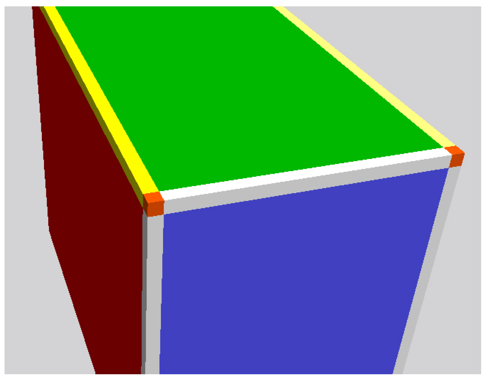
Abstract
:1. Introduction
1.1. Scope
1.2. Outline
2. Thermodynamics
2.1. Mathematical Thermodynamics
Thermodynamic Potentials
2.2. Scalar Potentials, Gradients, and Forces
2.3. The Internal Energy of an Empty Box
Entropy—More than Statistics
3. Chopping the Box—Quantization of Space
- bulk voxels,
- face voxels,
- edge voxels,
- vertex voxels.
4. Applications of the Quantized Box Model
4.1. Thermodynamics of Geometric Objects
4.2. Dimensionless Entities
4.3. Squeezing the Box
Special Relativity
4.4. Evolution of the Box
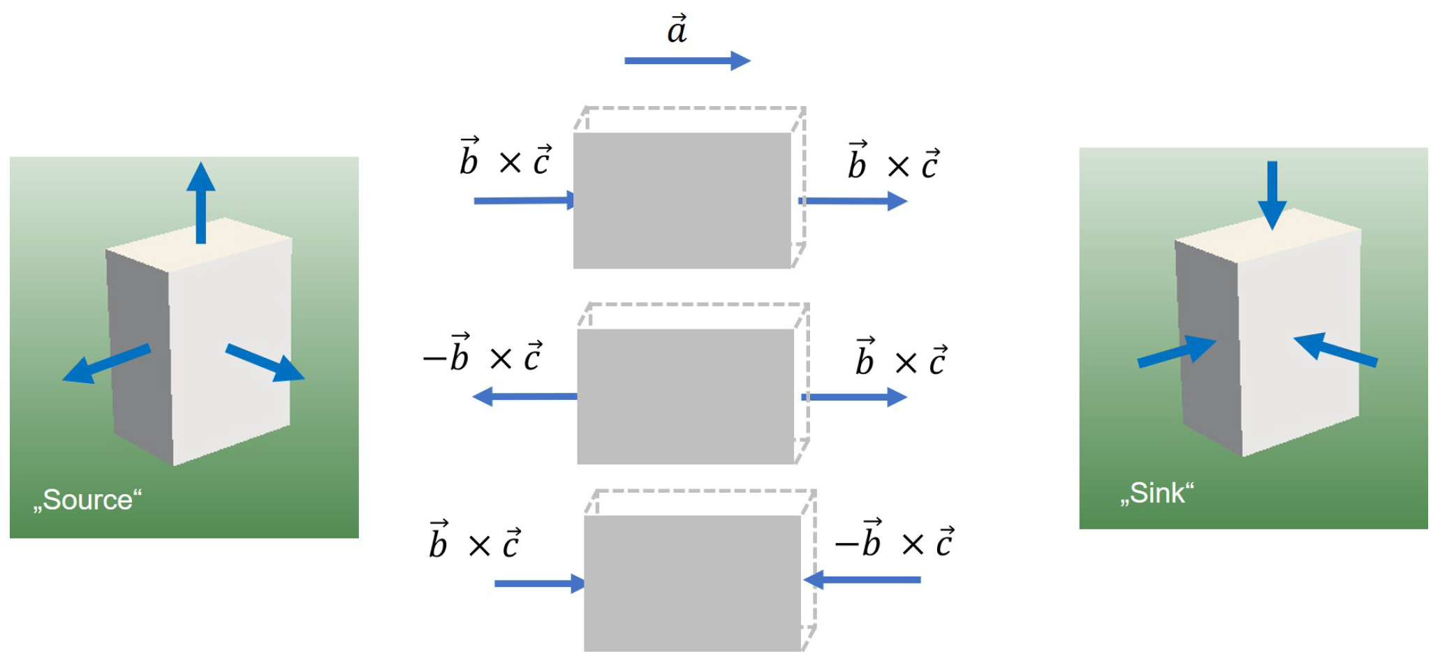
4.5. Translating the Box
4.5.1. Newton’s Laws
4.5.2. The Unruh Effect
4.5.3. Position-Dependent Volume
4.5.4. Uncertainty Relation
5. Beyond the Empty Box
- all three laws of Newton (classical mechanics),
- the harmonic oscillator equation,
- the Unruh equation,
- an uncertainty relation.
5.1. Oriented Surfaces
5.2. Shearing and Twisting the Box
5.3. Filling the Box
6. Summary and Outlook
Author Contributions
Funding
Institutional Review Board Statement
Data Availability Statement
Conflicts of Interest
Appendix A. Legendre Transformations
Appendix B. Relation between Dual-State Entropy and Boltzmann Entropy
References
- te Vrugt, M.; Needham, P.; Schmitz, G.J. Is thermodynamics fundamental? arXiv 2022, arXiv:2204.04352. [Google Scholar] [CrossRef]
- Jaynes, E.T. Probability Theory: The Logic of Science, 1st ed.; Cambridge University Press: Cambridge, UK, 2003. [Google Scholar]
- Doran, C.; Lasenby, A. Geometric Algebra for Physicists, 1st ed.; Cambridge University Press: Cambridge, UK, 2003. [Google Scholar]
- Bekenstein, J. Black holes and the second law. Lett. Nuovo C. 1972, 4, 737–740. [Google Scholar] [CrossRef]
- Schmitz, G.J. Entropy of Geometric Objects. Entropy 2018, 20, 453. [Google Scholar] [CrossRef] [PubMed]
- Planck, M. Eight Lectures on Theoretical Physics Delivered at Columbia University in 1909; Library of Alexandria, Columbia University Press: New York, NY, USA, 1915. [Google Scholar]
- Turner, M.S. Why Is the Temperature of the Universe 2.726 Kelvin? Science 1993, 262, 861–867. [Google Scholar] [CrossRef]
- Valery, A.R.; Dmitry, S.G. Introduction to the Theory of the Early Universe: Hot Big Bang Theory; World Scientific Publishing Company: Singapore, 2011. [Google Scholar]
- Lemaître, G. Un univers homogène de masse constante et de rayon croissant rendant compte de la vitesse radiale des nébuleuses extra-galactiques. Ann. Soc. Sci. Brux. 1927, 47, 49–59. [Google Scholar]
- Friedman, A. Über die Krümmung des Raumes. Z. Physik. 1922, 10, 377–386. [Google Scholar] [CrossRef]
- Verlinde, E. On the Origin of Gravity and the Laws of Newton. J. High Energy Phys. 2011, 2011, 29. [Google Scholar] [CrossRef]
- Kepler, J. Epitome Astronomiae Copernicanae; Johann Planck: Linz, Austria, 1618. [Google Scholar]
- Schwarzschild, K. Über das Gravitationsfeld einer Kugel aus inkompressibler Flüssigkeit nach der Einsteinschen Theorie. Sitzungsber. Preuss. Akad. Wiss. Berlin 1916, 189–196. [Google Scholar]
- Einstein, A. Über die Spezielle und die Allgemeine Relativitätstheorie, 24th ed.; Springer: Berlin, Germany, 2009. [Google Scholar]
- t’Hooft, G. Dimensional Reduction in Quantum Gravity. arXiv 2009, arXiv:gr-qc/9310026. [Google Scholar] [CrossRef]
- Bransden, B.; Joachain, C. Quantum Mechanics, 2nd ed.; Prentice Hall: Harlow, UK, 2000. [Google Scholar]
- Planck, M. Ueber das Gesetz der Energieverteilung im Normalspectrum. Ann. Phys. 1901, 309, 553–563. [Google Scholar] [CrossRef]
- Binasch, G.; Grünberg, P.; Saurenbach, F.; Zinn, W. Enhanced magnetoresistance in layered magnetic structures with antiferromagnetic interlayer exchange. Phys. Rev. B 1989, 39, 4828–4830. [Google Scholar] [CrossRef]
- von Weizsäcker, C.F. Zur Theorie der Kernmassen. Z. Phys. 1935, 96, 431–458. [Google Scholar] [CrossRef]
- Bekenstein, J.D. Bekenstein-Hawking entropy. Scholarpedia 2008, 3, 7375. [Google Scholar] [CrossRef]
- Schmitz, G.J. Thermodynamics of Diffuse Interfaces. In Interface and Transport Dynamics; Emmerich, H., Nestler, B., Schreckenberg, M., Eds.; Springer: Berlin, Germany, 2003; pp. 47–64. [Google Scholar]
- Crispino, L.C.B.; Higuchi, A.; Matsas, G.E.A. The Unruh effect and its applications. Rev. Mod. Phys. 2008, 80, 787–838. [Google Scholar] [CrossRef]
- Barceló, C.; Liberati, S.; Visser, M. Analogue gravity. Living Rev. Relativ. 2011, 14, 3. [Google Scholar] [CrossRef] [PubMed]
- te Vrugt, M.; Frohoff-Hülsmann, T.; Heifetz, E.; Thiele, U.; Wittkowski, R. From a microscopic inertial active matter model to the Schrödinger equation. Nat. Commun. 2023; in press. [Google Scholar] [CrossRef]
- Gibbs, J.W. On the Equilibrium of Heterogeneous Substances: First Part. Trans. Conn. Acad. Arts Sci. 1878, 3, 108–248. [Google Scholar]
- Gibbs, J.W. On the Equilibrium of Heterogeneous Substances: Second Part. Trans. Conn. Acad. Arts Sci. 1878, 3, 343–524. [Google Scholar]
- Gibbs, J.W. Elementary Principles in Statistical Mechanics; John Wilson and Son: Cambridge, MA, USA, 1902. [Google Scholar]
- Guggenheim, E. Modern Thermodynamics by the Methods of Willard Gibbs. J. Phys. Chem. 1934, 38, 713. [Google Scholar] [CrossRef]
- Gibbs, J. On the Fundamental Formula of Statistical Mechanics, with Applications to Astronomy and Thermodynamics (Abstract). Proc. Amer. Assoc. Adv. Sci. 1884, XXXIII, 57–58. [Google Scholar]
- Lukas, H.; Fries, S.G.; Sundman, B. Computational Thermodynamics: The Calphad Method, 1st ed.; Cambridge University Press: Cambridge, UK, 2007. [Google Scholar]
- Andersson, J.O.; Helander, T.; Höglund, L.; Shi, P.; Sundman, B. Thermo-Calc & DICTRA, computational tools for materials science. Calphad 2002, 26, 273–312. [Google Scholar] [CrossRef]
- Bale, C.; Bélisle, E.; Chartrand, P.; Decterov, S.; Eriksson, G.; Gheribi, A.; Hack, K.; Jung, I.H.; Kang, Y.B.; Melançon, J.; et al. FactSage thermochemical software and databases, 2010–2016. Calphad 2016, 54, 35–53. [Google Scholar] [CrossRef]
- Chen, S.L.; Daniel, S.; Zhang, F.; Chang, Y.; Yan, X.Y.; Xie, F.Y.; Schmid-Fetzer, R.; Oates, W. The PANDAT software package and its applications. Calphad 2002, 26, 175–188. [Google Scholar] [CrossRef]
- Saunders, N.; Guo, U.; Li, X.; Miodownik, A.; Schillé, J.P. Using JMatPro to model materials properties and behavior. JOM 2003, 55, 60–65. [Google Scholar] [CrossRef]
- Wallace, D. Thermodynamics as control theory. Entropy 2014, 16, 699–725. [Google Scholar] [CrossRef] [Green Version]
- Myrvold, W.C. The Science of ΘΔcs. Found. Phys. 2020, 50, 1219–1251. [Google Scholar] [CrossRef]
- Myrvold, W.C. Beyond Chance and Credence: A Theory of Hybrid Probabilities, 1st ed.; Oxford University Press: Oxford, UK, 2021. [Google Scholar]
- Callen, H.B. Thermodynamics and an Introduction to Thermostatistics, 2nd ed.; Wiley: New York, NY, USA, 1991. [Google Scholar]
- Elder, K.; Provatas, N. Phase-Field Methods in Materials Science and Engineering; Wiley-VCH: Weinheim, Germany, 2010. [Google Scholar]
- MICRESS®—The MICRostructure Evolution Simulation Software. Available online: https://micress.rwth-aachen.de/ (accessed on 12 June 2022).
- Schmitz, G.J.; Böttger, B.; Eiken, J.; Apel, M.; Viardin, A.; Carré, A.; Laschet, G. Phase-field based simulation of microstructure evolution in technical alloy grades. Int. J. Adv. Eng. Sci. Appl. Math. 2010, 2, 126–139. [Google Scholar] [CrossRef]
- Okano, A.; Matsumoto, T.; Kato, T. Gaussian Curvature Entropy for Curved Surface Shape Generation. Entropy 2020, 22, 353. [Google Scholar] [CrossRef]
- Schmitz, G.J. A phase-field perspective on mereotopology. AppliedMath 2022, 2, 54–103. [Google Scholar] [CrossRef]
- Gibbs, J.W. A Method of Geometrical Representation of the Thermodynamic Properties of Substances by Means of Surfaces. Trans. Conn. Acad. Arts Sci. 1873, 2, 309–342. [Google Scholar]
- Gibbs, J.W. Graphical Methods in the Thermodynamics of Fluids. Trans. Conn. Acad. Arts Sci. 1873, 2, 309–342. [Google Scholar]
- Ram, B. Engineering Mathematics, 1st ed.; Pearson: New Dehli, India, 2009. [Google Scholar]
- Noether, E. Invariante Variationsprobleme. Nachr. Ges. Wiss. Gott. Math.-Phys. Kl. 1918, 235–257. [Google Scholar]
- Hermann, S.; Schmidt, M. Noether’s theorem in statistical mechanics. Commun. Phys. 2021, 4, 176. [Google Scholar] [CrossRef]
- Mori, H. Transport, Collective motion, and Brownian motion. Prog. Theor. Phys. 1965, 33, 423–455. [Google Scholar] [CrossRef]
- Zwanzig, R. Ensemble Method in the Theory of Irreversibility. J. Chem. Phys. 1960, 33, 1338–1341. [Google Scholar] [CrossRef]
- te Vrugt, M.; Wittkowski, R. Mori-Zwanzig projection operator formalism for far-from-equilibrium systems with time-dependent Hamiltonians. Phys. Rev. E 2019, 99, 062118. [Google Scholar] [CrossRef]
- te Vrugt, M.; Wittkowski, R. Projection operators in statistical mechanics: A pedagogical approach. Eur. J. Phys. 2020, 41, 045101. [Google Scholar] [CrossRef]
- Camargo, D.; de la Torre, J.A.; Duque-Zumajo, D.; Español, P.; Delgado-Buscalioni, R.; Chejne, F. Nanoscale hydrodynamics near solids. J. Chem. Phys. 2018, 148. [Google Scholar] [CrossRef] [Green Version]
- Treumann, R.A.; Baumjohann, W. A note on the entropy force in kinetic theory and black holes. Entropy 2019, 21, 716. [Google Scholar] [CrossRef] [PubMed]
- Shannon, C.E. A mathematical theory of communication. Bell Syst. Tech. J. 1948, 27, 379–423. [Google Scholar] [CrossRef]
- Frigg, R. A field guide to recent work on the foundations of statistical mechanics. In The Ashgate Companion to Contemporary Philosophy of Physics; Rickles, D., Ed.; Ashgate: London, UK, 2008; pp. 99–196. [Google Scholar]
- Bronstein, I.N.; Semendyayev, K.A.; Musiol, G.; Muehlig, H. Handbook of Mathematics, 5th ed.; Springer: Berlin, Germany, 2007. [Google Scholar]
- Hahn, T.; Wigger, D.; Kuhn, T. Entropy Dynamics of Phonon Quantum States Generated by Optical Excitation of a Two-Level System. Entropy 2020, 22, 286. [Google Scholar] [CrossRef]
- Schmitz, G.J. Quantitative mereology: An essay to align physics laws with a philosophical concept. Phys. Essays 2020, 33, 479–488. [Google Scholar] [CrossRef]
- Gerla, G.; Mirandam, A. Mathematical Features of Whitehead’s Point-free Geometry. Handb. Whiteheadian Process Thought 2008, II, 119–129. [Google Scholar]
- Roeper, P. Region-Based Topology. J. Philos. Log. 1997, 26, 251–309. [Google Scholar] [CrossRef]
- Johnstone, P.T. The point of pointless topologies. Bull. Am. Math. Soc. 1983, 8, 41–53. [Google Scholar]
- Cullity, B.D.; Stock, S.R. Elements of X-ray Diffraction, 3rd ed.; Pearson Education Limited: Harlow, UK, 2014. [Google Scholar]
- Siqveland, L.M.; Skjaeveland, S.M. Derivations of the Young-Laplace equation. Capillarity 2021, 4, 23–30. [Google Scholar] [CrossRef]
- Greaves, G.; Greer, A.; Lakes, R.; Rouxel, T. Poisson’s ratio and modern materials. Nat. Mater. 2011, 10, 823–837. [Google Scholar] [CrossRef]
- Tiesinga, E.; Mohr, P.J.; Newell, D.B.; Taylor, B.N. CODATA Recommended Values of the Fundamental Physical Constants: 2018. J. Phys. Chem. Ref. Data 2021, 50, 033105. [Google Scholar] [CrossRef]
- Gibson, J.G. Alpha and electroweak coupling. arXiv 2001, arXiv:quant-ph/0112033. [Google Scholar] [CrossRef]
- Akarsu, Ö.; Kılınç, C.B. Bianchi type III models with anisotropic dark energy. Gen. Relativ. Gravit. 2010, 42, 763–775. [Google Scholar] [CrossRef]
- te Vrugt, M.; Hossenfelder, S.; Wittkowski, R. Mori-Zwanzig formalism for general relativity: A new approach to the averaging problem. Phys. Rev. Lett. 2021, 127, 231101. [Google Scholar] [CrossRef] [PubMed]
- Le Delliou, M.; Deliyergiyev, M.; del Popolo, A. An Anisotropic Model for the Universe. Symmetry 2020, 12, 1741. [Google Scholar] [CrossRef]
- Larena, J.; Alimi, J.M.; Buchert, T.; Kunz, M.; Corasaniti, P.S. Testing backreaction effects with observations. Phys. Rev. D 2009, 79, 083011. [Google Scholar] [CrossRef]
- Buchert, T.; Carfora, M.; Ellis, G.F.R.; Kolb, E.W.; MacCallum, M.A.H.; Ostrowski, J.J.; Räsänen, S.; Roukema, B.F.; Andersson, L.; Coley, A.A.; et al. Is there proof that backreaction of inhomogeneities is irrelevant in cosmology? Class. Quantum Grav. 2015, 32, 215021. [Google Scholar] [CrossRef]
- Brown, H.R. Physical Relativity: Space-Time Structure from a Dynamical Perspective; Clarendon Press: Oxford, UK, 2005. [Google Scholar]
- Ghedini, E.; Friis, J.; Goldbeck, G.; Hashibon, A.; Schmitz, G.J.; Moruzzi, S.; Varzi, A.C. The Elementary Multiperspective Material Ontology. 2022; Unpublished Work. [Google Scholar]
- Ferretti, E. The Cell Method: An Enriched Description of Physics Starting from the Algebraic Formulation. Comput. Mater. Contin. 2013, 36, 49–71. [Google Scholar] [CrossRef]
- Atkins, P.; Friedman, R. Molecular Quantum Mechanics, 5th ed.; Oxford University Press: Oxford, UK, 2011. [Google Scholar]
- Liu, Z.K. Theory of cross phenomena and their coefficients beyond Onsager theorem. Mater. Res. Lett. 2022, 10, 393–439. [Google Scholar] [CrossRef]


Disclaimer/Publisher’s Note: The statements, opinions and data contained in all publications are solely those of the individual author(s) and contributor(s) and not of MDPI and/or the editor(s). MDPI and/or the editor(s) disclaim responsibility for any injury to people or property resulting from any ideas, methods, instructions or products referred to in the content. |
© 2023 by the authors. Licensee MDPI, Basel, Switzerland. This article is an open access article distributed under the terms and conditions of the Creative Commons Attribution (CC BY) license (https://creativecommons.org/licenses/by/4.0/).
Share and Cite
Schmitz, G.J.; te Vrugt, M.; Haug-Warberg, T.; Ellingsen, L.; Needham, P.; Wittkowski, R. Thermodynamics of an Empty Box. Entropy 2023, 25, 315. https://doi.org/10.3390/e25020315
Schmitz GJ, te Vrugt M, Haug-Warberg T, Ellingsen L, Needham P, Wittkowski R. Thermodynamics of an Empty Box. Entropy. 2023; 25(2):315. https://doi.org/10.3390/e25020315
Chicago/Turabian StyleSchmitz, Georg J., Michael te Vrugt, Tore Haug-Warberg, Lodin Ellingsen, Paul Needham, and Raphael Wittkowski. 2023. "Thermodynamics of an Empty Box" Entropy 25, no. 2: 315. https://doi.org/10.3390/e25020315