
Investigating Deep Stock Market Forecasting with Sentiment Analysis

Department of Mathematics, University of Patras, 26504 Patras, Greece
*
Authors to whom correspondence should be addressed.
Entropy 2023, 25(2), 219; https://doi.org/10.3390/e25020219
Submission received: 13 December 2022
/
Revised: 14 January 2023
/
Accepted: 20 January 2023
/
Published: 23 January 2023
(This article belongs to the Special Issue Recent Trends and Developments in Econophysics)
Abstract
:When forecasting financial time series, incorporating relevant sentiment analysis data into the feature space is a common assumption to increase the capacities of the model. In addition, deep learning architectures and state-of-the-art schemes are increasingly used due to their efficiency. This work compares state-of-the-art methods in financial time series forecasting incorporating sentiment analysis. Through an extensive experimental process, 67 different feature setups consisting of stock closing prices and sentiment scores were tested on a variety of different datasets and metrics. In total, 30 state-of-the-art algorithmic schemes were used over two case studies: one comparing methods and one comparing input feature setups. The aggregated results indicate, on the one hand, the prevalence of a proposed method and, on the other, a conditional improvement in model efficiency after the incorporation of sentiment setups in certain forecast time frames.
1. Introduction
Somewhere in the course of history, the human species’ need for knowledge of possible future outcomes of various events emerged. Associative norms were thus constructed between decision-making and observed data that were influenced by theoretical biases that had been inductively established on the basis of such observations. Protoscience was formed. Or not?
Even if this hypothetical description of human initiation into scientific capacities is naive or even unfounded, the bottom line is that the human species partly operates on the basis of predictions. Observing time-evolving phenomena and questioning their structure in the direction of an understanding that will derive predictions about their projected future behavior constitutes an inherent part of post-primitive human history. In response to this self-referential demand and assuming that the authors are post-primitive individuals, the core of the present work is about predicting sequential and time-dependent phenomena. This domain is called time series forecasting. Time series forecasting is, in broad terms, the process of using a model to predict future values of variables that characterize a phenomenon based on historical data. A time series is a set of time-dependent observations sampled at specific points in time. The sampling rate depends on the nature of the problem. Moreover, depending on the number of variables describing the sequentially recorded observations, a distinction is made between univariate and multivariate time series. Since there is a wide range of time-evolving problems, the field is quite relevant in modern times, with an increasing demand for model accuracy and robustness.
In addition, there are phenomena, the mathematical formalism of which is represented by time series with values which are also sub-determined by the given composition of a society of individuals. This means that the attitudes of such individuals, as they nonetheless form within the whole, are somewhat informative about aspects of the phenomenon in question. It is natural, given human nature and the consequent conceptual treatment of the world as part of it, that these attitudes are articulated somewhere linguistically. Therefore, a hypothesis on which mathematical quantifications of the attitudes of which such linguistic representations that are signs are possible could, if valid, describe a framework for improving the modeling of the phenomena in question. For example, specific economic figures can be points in a context, the elements of which are partially shaped by what is said about them. Accordingly, it can be argued that a line of research that would investigate whether stock closing prices can be modeled in terms of their future fluctuations using relevant linguistic data collected from social networks is valid.
Thus, in this work, the incorporation of sentiment analysis in stock market forecasting is investigated. In particular, a large number of state-of-the-art methods are put under an experimental framework that includes multiple configurations of input features that incorporate quantified values of sentiment attitudes in the form of time series. These time series consist of sentiment scores extracted from Twitter using three different sentiment analysis methods. Regarding prediction methods, there are schemes that come from both the field of statistics and machine learning. Within the machine learning domain, deep learning and other state-of-the-art methods are currently in use, dominating research. Here, a large number of such widely used state-of-the-art models were benchmarked in terms of performance. Moreover, various sentiment setups of input features were tested. Two distinct case studies were investigated. In the first case study, the evaluations were organized according to methods. The subsequent comparisons followed the grouping. In the second case study, the comparisons concerned the feature setups used as inputs. Sentiment scores were tested in the context of improving the predictive capacities of the various models used. All comparisons yielded results from an extended experimental procedure that incorporated various steps. The whole setting involved a wide range of multivariate setups, which included various sentiment time series. Multiple evaluation metrics and three different time frames were used to derive multiple-view results. Below, first, a brief presentation of related literature is given. Then, the experimental procedure is thoroughly presented, which is followed by the results. Finally, Section 5 lists the extracted conclusions.
2. Related Work
The continuous and ever-increasing demand for accurate forecasts across a wide range of human activity has been a key causal factor contributing to the unabated research activity occurring within the field of time series forecasting. Thus, the prediction of time series constitutes a strong pole of interest for the scientific community. Consequently, in recent decades, this interest has been reflected in a wealth of published work and important results. In this section, a brief presentation of relevant literature is given. Due to space constraints, this presentation is more indicative than exhaustive, and its purpose is just to provide a starting point for a more thorough and in-depth review.
A trivial way to distinguish the problems associated with time series forecasting would be to divide the task into two categories with respect to the type of final output. The first category includes problems where the goal is to predict whether a future value is expected to increase or decrease over a given time horizon. This task can essentially be treated as a binary classification problem. The second category includes tasks where the goal is to accurately predict the price of a time series in a specific time frame. Here, the output can take any value within a continuous interval, and hence, the prediction process can be treated as a regression problem. One can easily imagine that the difficulty of the problems belonging to the second category is greater than that of the first and that their treatment requires more complex and precise refinements. Apparently, interesting works can be found in both categories, but the context of this paper dictates a focus on the latter.
A subclass of problems regarding focus on the direction in which a time series will move features those involving the increase or decrease of closing price values of various stocks. In particular, in [1], an ensemble technique based on tree classifiers—specifically on random forests and gradient boosted decision trees—which predicts movement in various time frames is proposed. For the same purpose in [2], support vector machines (SVMs) are used in combination with sentiment analysis performed on data drawn from two forums considered to be the largest and most active mainstream communities in China. This paper is an attempt to predict stock price direction using SVMs and taking into account the so-called day-of-week effect. Adding sentiment variables results in up to 18% better predictions. Similar results, which indicate the superiority of SVMs compared to other classification algorithms, are also presented in [3], where well-known methods such as linear discriminant analysis, quadratic discriminant analysis, and Elman backpropagation neural networks are used for comparison. Encouraging results regarding the prediction of time series movement direction have also been achieved using hybrid methods, where modern schemes combining deep neural network architectures are applied to big data [4]—again—for the daily-based prediction of stock market prices. Regarding the second category, where the goal is to predict the specific future values of a time series and not merely its direction, the literature appears richer. This seems as if it is a fact rather expected if one takes into account the increased difficulty of the task and the high interest of the research community in pursuing the production of improved results. In the past decades, traditional statistical methods seemed to dominate the field of time series forecasting [5,6]. However, as expected, according to their general effectiveness, machine learning methods began to gain ground and dominate the field [7,8]. Traditional machine learning methods are incorporated in various time series forecasting tasks, such as using SVMs for economic data predictions [9] and short-term electric load forecasting [10], while architectures based on neural networks are also particularly popular. Regarding the latter—as this is probably the largest part of the literature regarding the use of machine learning in prediction problems—the use of such methods has covered a wide range of applications. Some indicative examples are the prediction of oil production [11] and traffic congestion [12] using deep LSTM recurrent networks, while an aggregated version of LSTMs has additionally been used for the short-term prediction of air pollution. Forecasting river water temperature using a hybrid model based on wavelet-neural network architecture was presented in [13], while recurrent neural networks (RNNs) have been deployed to forecast agricultural commodity prices in China [14]. Since the list of examples where neural network-based techniques show promise is long, the reader is urged to pursue additional personal research.
Furthermore, it is possibly worth mentioning the fact that in addition to increasingly sophisticated methods, techniques based on the theory of ensembles are also gaining ground. Roughly speaking, these are techniques in which the final result is derived through a process of using different models, with the prediction being formed from the combination of the individual ones. As an example, one can mention the ensemble scheme proposed in [15] for the prediction of energy consumption: it combines support vector regression (SVR), backpropagation neural network (BPNN), and linear regression (LR) learners. A similar endeavor is presented in [16], where an ensemble consisting of four learners, that is, long short-term memory (LSTM), gate recurrent unit (GRU), autoencoder LSTM (Auto-LSTM), and auto-GRU, is used for the prediction of solar energy production. A comparison involving over 300 individual and ensemble predictive layouts over Greek energy load data is presented in [17]. There, in addition to the large number of ensembles tested, the comparison also concerns both a number of forecast time frames as well as different modifications of the input data in various multivariate arrangements. In [18], an ensemble scheme based on linear regression (LR), support vector regression (SVR), and the M5P regression tree (M5PRT) is proposed to predict cases and deaths attributed to the COVID-19 pandemic regarding southern and central European countries.
With regard now to the context of this work, and given that its purpose—which is an extension of the work in [19]—is twofold, aiming, on the one hand, to compare a large number of methods and, on the other hand, to investigate the contribution of incorporating sentiment analysis into the forecasting process, it follows that a simple presentation of similarly targeted tasks seems quite essential. As for the first objective—that of comparing methods—there are several interesting works that have been carried out in recent years. In [20], the comparison between the traditional ARIMA method and LSTMs using economic data is investigated. A similar comparison between the two methods is implemented in [21], now aiming to predict bitcoin values, while in [22], the gated recurrent unit (GRU) scheme is also included in the comparison. Comparative works of the ARIMA method with various schemes have also been carried out, such as with neural network auto-regressive (NNAR) techniques [23], with the prophet method [24], with LSTMs and the XGBOOST method [25], as well as with wavelet neural network (WNN) and support vector machines (SVM) [26]. Although, in general, modern schemes tend to perform better than ARIMA, any absolute statement would not be representative of reality. Indeed, research focused on comprehensively reviewing the use of modern methods can provide a detailed overview of the relevant work to date. Indicatively, in [27], an extensive review of the use of artificial neural networks in time series forecasting is presented, covering studies published from 2006 onwards, over a decade. A similar survey covering the period from 2005 to 2019 and focusing on deep learning techniques with applications to financial data can be found in [28]. Furthermore, regarding the experimental evaluation of modern machine learning architectures, in [29], a thorough experimental comparison is presented, concerning seven different deep learning architectures applied to 12 different forecasting problems, using more than 50,000 time series. According to the implementation of more than 38000 models, it is argued that the architectures of LSTMs and CNNs outperform all others. In [30], the comparison of a number of methods—such as ARIMA, neural basis expansion analysis (NBEATS), and probabilistic methods based on deep learning models—applied to time series of financial data is presented. Additionally, in [31], a comparison between CNNs, LSTMs, and a hybrid model of them is given, which was deployed on data concerning the forecasting of the energy load coming from photovoltaics. There, the generated results, on the one hand, indicate the dominance of the hybrid model—emphasizing the necessity to create efficient combinatorial schemes—and, on the other, show that the models’ predictions improve by using a larger amount of data in the training set.
In relation to the second objective—which concerns the investigation of whether the use of information based on sentiment analysis regarding public opinion extracted from social networks favors the predictions—the available literature seems comparatively poorer but presents equally interesting results. The relationship between tweet board literature and financial market instruments is examined in [32], with results revealing a high correlation between stock prices and Twitter sentiments. In [33], using targeted topics to extract sentiment from social media, a model to predict stock price movement is presented. Moreover, the effectiveness of incorporating sentiment analysis into stock forecasting is demonstrated. In addition, ref. [34] is an attempt to capture the various relationships between news articles and stock trends using well-known machine learning techniques such as random forest and support vector machines. In [35], after assembling a financial-based sentiment analysis dictionary, a model incorporating the dictionary was developed and tested on data from the pharmaceutical market, exhibiting encouraging results. In [36], sentiment polarity is extracted by observing the logarithmic return of the ratio between the average stock price one minute before and one minute after the relevant stock’s news is published. Then, using RNNs and LSTMs, the direction of the stock is successfully predicted. The exploitation of sentiment analysis techniques has also been used to predict the stock market during health crises [37] such as H1N1 and, more recently, COVID-19. Possible links between social media posts and closing stock prices at specific time horizons were found. More specifically, for COVID-19, the polarity of the posts seemed to affect the stock prices after a period of about six days.
Regarding the prediction of various stock market closing prices—which is also the thematic center of this paper—in [38], data collected from Twitter are initially analyzed in terms of their sentiment scores and are then used to predict the movement of stock prices, using naive Bayes and multiclass SVM classifiers. A similar procedure was followed in [39], where least squares support vector regression (LSSVR) and backpropagation neural networks were deployed to predict the total monthly sales of vehicles in the USA, using additional sentiment information combined with historical sales data. Data collected from the online editions of international newspapers were used in [40] to predict the closing stock price values, incorporating both traditional methods, such as ARIMA, and newer ones, such as the Facebook prophet algorithm and RNN architectures that use as input both numerical values of the time series to be predicted as well as combinations of the polarity of extracted sentiments.
In [41], both traditional and modern machine learning methods such as support vector machines, linear regression, naive Bayes, and long short-term memory are used in combination with the incorporation of opinion data, current news, and past stock prices. In [42], sentiment analysis and empirical model decomposition are used so that complex time series can be broken down into simpler and easier to manage parts, together with an attention mechanism that attributes weight to the information considered most useful for the task being performed each time. A method based on the architecture of LSTMs that uses information derived from sentiment analysis together with multiple data sources is presented in [43]. Initially, textual data related to the stock in question are collected, and using methods based on convolutional neural network architectures, the polarity of investors’ sentiment is extracted. This information is then combined with that of the stock’s past closing prices and other technical indicators to produce the final forecast. In [44], a hybrid model that leverages deep learning architectures, such as convolutional neural networks, to extract and categorize investor sentiment as detected in financial forums is described. The extracted sentiments are then combined with information derived from technical financial indicators to predict future stock prices in real-world problems using LSTM architectures. SVM architectures are used on Twitter data to extract polarity in [45]. The extracted polarities are used in an incremental active learning scheme, where the continuous stream of content-changing tweets is used to predict the closing stock price of the stock market.
Sentiment analysis has also been used to predict the price of bitcoin in real time, using—and at the same time comparing—LSTM techniques and the classical ARIMA method [46], where the exploitation of the information derived from sentiment analysis has been beneficial. Similar research focused on predicting the price direction of the cryptocurrencies Bitcoin and Ethereum using sentiment analysis from data drawn from Twitter and Google Trends and given as input to a linear predictive model is presented in [47]. Interestingly, the volume of tweets affects the prediction to a greater extent than the polarity of the sentiment extracted from the tweets. Forecasting the price direction of four popular cryptocurrencies—Bitcoin, Ethereum, Ripple, and Litecoin—using machine learning techniques and data drawn from social networks is presented in [48]. Classical methods such as neural networks (NN), support vector machines (SVM), and random forests (RF) are compared. An interesting fact is that Twitter, roughly speaking, seems to favor the prediction of specific cryptocurrencies rather than all of them. Using sentiment analysis has also been beneficial in the field of cybersecurity. In [49], a methodology that exploits the knowledge of hacker behavior for predicting malicious events in cyberspace by performing sentiment analysis with different techniques (VADER, LIWC15, and SentiStrength) on data collected from hacking forums, both on the dark web and on the surface web, is presented.
The—rather diverse—list of applications in which the use of sentiment analysis techniques can improve the generated forecasts is proportional to the fields in which time series forecasting is applied since, in general, the utilization of public opinion knowledge appears to have a positive effect on the forecasting process. Some of them that have been implemented in the last five years have already been mentioned in passing, and many others can be added. Such would include predicting the course of epidemics, such as that of the Zika virus in the USA in 2016 [50] or the COVID-19 pandemic, the outcome of electoral contests [51], the prediction of the price of e-commerce products [52], and the list goes on. Given human nature and the consequent conceptual coping of the world by human subjects, sentiment analysis seems justifiably relevant in a multitude of applications. The reader is therefore encouraged to conduct additional bibliographic research.
3. Experimental Procedure
Information regarding the stages of the experimental procedure will now be presented. This presentation will be as detailed as possible given the necessary space constraints and content commitments in order not to disrupt the depictive nature of the paper.
It has already been mentioned that to some extent, the “core” of the present work consists of an experimental procedure that aims, in its most abstract scope, to check the efficiency, on the one hand, of a number of state-of-the-art algorithms and, on the other, of incorporating sentiment analysis into predictive schemas. Thus, a total of 16 datasets × 67 combinations × 30 algorithms × 3 time-shifts = 96,480 experiments were conducted. The dataset consisted of time series containing the daily closing values of various stocks along with a multitude of 67 different sentiment score setups. Specifically, 16 datasets of stocks containing such closing price values were used over a three-year period, beginning on 2 January 2018 and ending on 24 December 2020. Generated sentiment scores from relevant textual data extracted from the Twitter microblogging platform were used. Three different sentiment analysis methods were deployed. The sentiment score time series and the closing values were subjected to a 7-day and a 14-day rolling mean strategy, yielding a total of 12 distinct features. Various combinations of the created features resulted in a total of 67 distinct input setups per algorithm. The calculated sentiment scores along with the closing values were then tested under both univariate and multivariate forecasting schemes. Lastly, 30 state-of-the-art methods were investigated. Below, a more thorough presentation of the aforementioned experimental setting follows.
3.1. Datasets
Starting with data, the process of collecting and creating the sets used will now be addressed.
3.1.1. Overview
To begin with, Table 1 contains the names of the aforementioned datasets along with their corresponding abbreviations. These initial data included time series containing closing values for 16 well-known listed companies. All sets comprise three-year period data for dates ranging from 2 January 2018 to 24 December 2020.
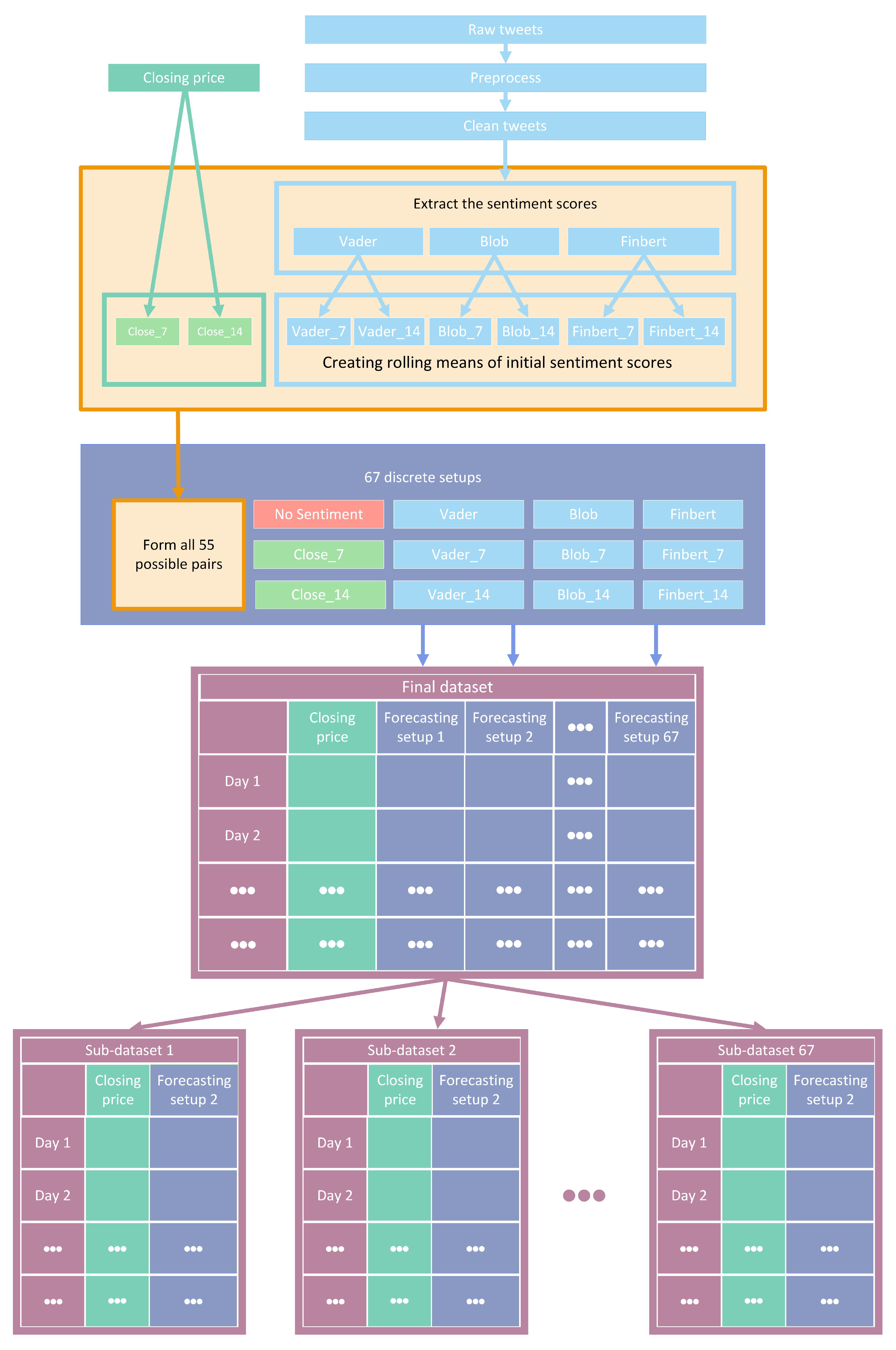
Essentially, the initial features were four: that is, the closing prices of each stock and three additional time series containing relative sentiment scores for the given period. Subsequently, and after applying 7- and 14-day rolling averages, a total of 14 features were extracted. Thus, for each share, the final input settings were composed by introducing altered features derived from stock values and a sentiment analysis process applied to an extended corpus of tweets. Figure 1 depicts a—rather abstractive—snapshot of the whole process from data collection to the creation of the final input setups.
3.1.2. Tweets and Preprocessing
A large part of the process involved deriving sentiment scores related to stocks. Using the Twitter Intelligence Tool (TWINT) [53], a large number of stock-related posts written in English were downloaded from Twitter and grouped by day. TWINT is an easy-to-use yet sophisticated Python-based Twitter scraping tool. After a comprehensive search for stock-related remarks that were either directly or indirectly linked to shares under consideration, a sizable amount of text data containing daily attitudes toward stocks were created. Then, the collected textual sets underwent the various preprocessing procedures necessary in order to be passed on to the classification modules for extracting their respective sentiment scores.
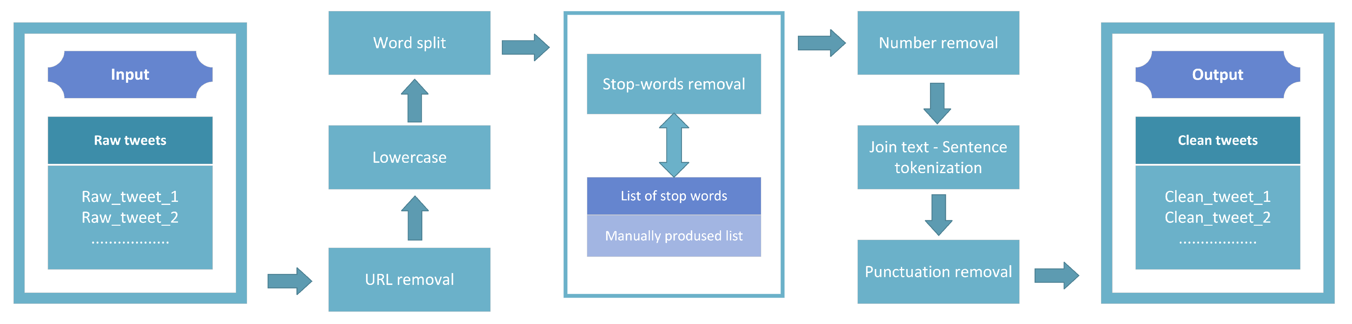
Regarding preprocessing tweets, initially, irrelevant hyperlinks and URLs were removed using the Re Python library [54]. Each tweet was then converted to lowercase and split into words. Then, unwanted phrases from a manually produced list and various numerical strings were also dismissed. After performing the necessary joins to restore each text to its original structure, each tweet was tokenized in terms of its sentences using the NLTK [55,56] library. Lastly, using the String [57] module, punctuation removal was applied. The whole text-preprocessing step is schematically presented in Figure 2.
3.1.3. Sentiment Analysis
The subsequent process involved extracting sentiment scores from the gathered yet cleaned tweets. To perform the sentiment quantification step, three different sentiment analysis methods were utilized.
Specifically, the procedure included extracting sentiment scores from TextBlob [58], using the Vader sentiment analysis tool [59], and incorporating FinBERT [60]. FinBERT is a financial-based fine-tuning of the BERT [61] language representation model. Using each of the above methods, daily sentiment scores were extracted for each stock. The daily mean was then extracted, forming the final collection, which constituted the sentiment-valued time series of every corresponding method. Then, 7- and 14-day moving averages were applied to the previously extracted sentiment score time series. This resulted in the extraction of nine sentiment time series, which, together with the application of the aforementioned procedure to the closing price time series, led to the final number of 12 generated time series used as features. Various combinations of the above features, along with the univariate case scenario, resulted in 67 different study cases. These data constituted the distinct experimental procedures that run for every algorithm. The use of three different methods of sentiment analysis has already been mentioned. Below, a rough description of these methods is given. For further information, the reader is advised to refer to the respective papers.
- TextBlob: The TextBlob module is a Python-based library for performing a wide range of manipulations over text data. The specific TextBlob method used in this work is a rule-based sentiment-analysis scheme. That is, it works by simply applying manually created rules. This is how the value attributed to the corresponding sentiment score is calculated. An exemplified snapshot of the process would be counting the number of times a term of interest appears within a given section. This would modify the projected sentiment score values in line with the way the phrase is assessed. Here, within this experimental setup and by exploiting TextBlob’s sentiment property, a real number within the interval representing the sentiment polarity score was generated for each tweet. The algorithm’s numerical output was then averaged using the individual scores of each tweet to obtain a single sentiment value representing the users’ daily attitudes;
- Vader: Vader is also a straightforward rule-based approach for realizing general sentiment analysis. In the context of this work, the Vader sentiment analysis tool was used in order to extract a compound score produced by a normalization of sentiment values that the algorithm calculates. Specifically, given a string, the procedure outputs four values: negative, neutral, and positive sentiment values, as well as the aforementioned composite score used. A normalized average of all compound scores for each day was generated the usual way. The resulting time series contained daily sentiment scores that ranged within the interval;
- FinBERT: Regarding FinBERT, in this work, the implementation contained in [62] was utilized. Specifically, the model that was trained on PhraseBank presented in [63] was used. Again, first, the daily scores regarding sentiment attitudes were extracted to eventually form a daily average time series. Generally, the method is a pre-trained natural-language-processing (NLP) model for sentiment analysis. It is produced by simply fine-tuning the pre-trained BERT model over financial textual data. BERT, meaning bidirectional encoder representations from transformers, is an implementation of the transformers architecture used for natural language processing problems. The technique is basically a pre-trained representational model based on transfer learning principles. Given textual data, multi-layer deep representations are trained with a bidirectional attention strategy so that the various different contexts of each linguistic token constitute the content of the token’s embedding. Regardless of data references—here financial—the model can be fine-tuned in any domain by only using a single additional layer that addresses the specific tasks.
3.2. Algorithms
In this section, the methods, algorithmic schemes, and architectures employed in the experiments are listed. Additional details are given on the implementation framework and the tools used.
Regarding the algorithms used, a total of 30 different state-of-the-art methods and method variations were compared. The number of 30 methods used results from the supplementation of the set of well-known core methods with their variations. Further details can be found in the cited tsAI library [64], using which the implementation was carried out. However, it is this multitude of methods that apparently makes a detailed presentation practically impossible. Nevertheless, the reader is urged to track the cited papers. Table 2 contains the main algorithms utilized during the experimental procedure along with a corresponding citation. There, among others, one can notice that in addition to a multitude of state-of-the-art methods, implementations involving combinations of the individual architectures were also used. Note that in addition to the corresponding papers, information regarding the variations of the basic algorithms employed can be searched, inter alia, in notebook files taken from the library implementations.
In order to carry out the experiments, the Python library tsAI [64] was used. The tsAI module is “an open-source deep learning package built on top of Pytorch and Fastai focused on state-of-the-art techniques for time series tasks like classification, regression, forecasting” [64], and others. Here, the forecasting procedure was essentially treated as a predictive regression problem. In the experiments, the initial parameters of the respective methods from the library were preserved with the implementation environment being kept fixed for all algorithmic schemes. Thus, all algorithms compared were utilized in the most basic configuration. That way, one can gain additional insight regarding implementing high-level yet low-code programming and data analysis in real-world tasks. Of the data, 20% were used as the test set. Regarding prediction time horizons, three forecast scenarios were implemented: one single-step and two multi-step. In particular, with regard to multi-step forecasts, and leaving aside the single-step predictions, estimates were provided for a seven-day window on the one hand and a fourteen-day window on the other. The results were evaluated according to the metrics presented in the following paragraph.

Table 2.
Algorithms.
| No. | Abbreviation | Algorithm 1 |
|---|---|---|
| 1 | FCN | Fully Convolutional Network [65] |
| 2 | FCNPlus | Fully Convolutional Network Plus [66] |
| 3 | IT | Inception Time [67] |
| 4 | ITPlus | Inception Time Plus [68] |
| 5 | MLP | Multilayer Perceptron [65] |
| 6 | RNN | Recurrent Neural Network [69] |
| 7 | LSTM | Long Short-Term Memory [70] |
| 8 | GRU | Gated Recurrent Unit [71] |
| 9 | RNNPlus | Recurrent Neural Network Plus [69] |
| 10 | LSTMPus | Long Short-Term Memory Plus [69] |
| 11 | GRUPlus | Gated Recurrent Unit Plus [69] |
| 12 | RNN_FCN | Recurrent Neural—Fully Convolutional Network [72] |
| 13 | LSTM_FCN | Long Short-Term Memory—Fully Convolutional Network [73] |
| 14 | GRU_FCN | Gated Recurrent Unit—Fully Convolutional Network [74] |
| 15 | RNN_FCNPlus | Recurrent Neural—Fully Convolutional Network Plus [75] |
| 16 | LSTM_FCNPlus | Long Short-Term Memory—Fully Convolutional Network Plus [75] |
| 17 | GRU_FCNPlus | Gated Recurrent Unit—Fully Convolutional Network Plus [75] |
| 18 | ResCNN | Residual—Convolutional Neural Network [76] |
| 19 | ResNet | Residual Network [65] |
| 20 | RestNetPlus | Residual Network Plus [77] |
| 21 | TCN | Temporal Convolutional Network [78] |
| 22 | TST | Time Series Transformer [79] |
| 23 | TSTPlus | Time Series Transformer Plus [80] |
| 24 | TSiTPlus | Time Series Vision Transformer Plus [81] |
| 25 | Transformer | Transformer Model [82] |
| 26 | XCM | Explainable Convolutional Neural Network [83] |
| 27 | XCMPlus | Explainable Convolutional Neural Network Plus [84] |
| 28 | XceptionTime | Xception Time Model [85] |
| 29 | XceptionTimePlus | Xception Time Plus [86] |
| 30 | OmniScaleCNN | Omni-Scale 1D-Convolutional Neural Network [87] |
1 Methods and method variations used.
3.3. Metrics
Regarding performance evaluation, six metrics were used. The use of the different metrics serves the necessity of having not only a presentation of the conclusions of a large comparison of methods and feature and sentiment setups but also a number of diverse extractions in terms of evaluation aspects that can be used in future research. This is exactly because each of the metrics exposes the results in different aspects, and therefore, an investigation would be incomplete if it focused on just one of them. Thus, regarding evaluating results, each one of the six performance indicators utilized has advantages and disadvantages. The metrics used are:
- the Mean Absolute Error (MAE);
- the Mean Absolute Percentage Error (MAPE);
- the Mean Squared Error (MSE);
- the Root Mean Squared Error (RMSE);
- the Root Mean Squared Logarithmic Error (RMSLE);
- the Coefficient of Determination .
In what follows, a rather detailed description of aspects of the aforementioned well-known evaluation metrics is given. The presentation aspires to provide details and some insight regarding the interpretation of the metrics. Below, the actual values are denoted by and the forecasts are denoted by .
3.3.1. MAE
First is MAE:
MAE stands for the arithmetic mean of the absolute errors, and it is a very straightforward metric and easy to calculate. By default, in terms of the difference between the prediction and the observation, the values share the same weights. The absence of exponents in the analytic form ensures good behavior, which is displayed even when outliers are present. The target variable’s unit of measurement is the one expressing the results. MAE is a scale-dependent error metric; that is, the scale of the observation is crucial. This means that it can only be used to compare methods in scenarios where every scheme incorporates the same specific target variable rather than different ones.
3.3.2. MAPE
Next is MAPE:
MAPE is the mean absolute percentage error. It is a relative and not an absolute error measure. MAPE is common when evaluating the accuracy of forecasts. It is the average of the absolute differences between the prediction and the observations divided by the absolute value of the observation. A multiplication by 100 can afterwards convert this output to a percentage. This error cannot be calculated when the actual value is zero. Instead of being a percentage, in practice, it can take values in . Specifically, when the predictions contain values much larger than the observations, then the MAPE output can exceed . Conversely, in cases where both the prediction and the observation contain low values, the output of the metric may deviate greatly from . This, in turn, can lead to a misjudgment of the model’s predictive capabilities, believing them to be limited when, in fact, the errors may be low. MAPE attributes more weight to cases where the predicted value is higher than the actual one. These cases produce larger errors. Hence, using this metric is best suitable for methods with low prediction values. Lastly, MAPE, being not scale-dependent, can be used to evaluate comparisons of a variety of different time series and variables.
3.3.3. MSE
The next metric is MSE:
MSE stands for mean squared error. It constitutes a common forecast evaluation metric. The mean squared error is the average of the squares of the differences between the actual and predicted values. Its unit of measurement is the square of the unit of the variable of interest. Looking at the analytical form, first, the square of the differences ensures the non-negativity of the error. At the same time, it makes information about minor errors usable. It is obvious, at the same time, that larger deviations entail larger penalties, i.e., a higher MSE. Thus, outliers have a big influence on the output of the error; that is, the existence of such extreme values has a significant impact on the measurements and, consequently, the evaluation. Furthermore, and in a sense the other way around, when differences are less than 1, there is a risk of overestimating the predictive capabilities of the model. Given the error’s differentiability, as one can observe, it can easily be optimized.
3.3.4. RMSE
Moving on to RMSE:
RMSE stands for root mean squared error. It is a common metric for evaluating differences between estimated values and observations. To compute it, apparently, one just calculates the root of the mean squared error. From the numerical formulation, one can think of the metric as an abstraction that captures the representation of something of an average distance between the actual values and the predictions. That is, if one ignores the denominator, then one can observe the formula as being the Euclidean distance. The subsequent interpretation of the metric as a kind of normalized distance comes out of the act of division by the number of observations. Here also, the existence of outliers has a significant impact on the output. In terms of interpreting error values, the RMSE is expressed in the same units as the target variable and not in its square, as in the MSE, making its use straightforward. Finally, the metric is scale-dependent; hence, one can only use it to evaluate various models or model variations given a particular fixed variable.
3.3.5. RMSLE
The next metric is also an error. The formula for RMSLE is as follows:
RMSLE stands for Root Mean Squared Logarithmic Error. The RMSLE metric seems as if it is a modified version of the MSE. Using this modification is preferred when predictions display significant deviations. RMSLE uses logarithms of both the observations and predicted values while ensuring non-zero values in the logarithms through the appropriate simple unit additions appearing in the formula. This modified version is resistant to the existence of outliers and noise, and it smooths the penalty that the MSE imposes in cases in which predictions deviate significantly from observations. The metric cannot be used when there are negative values. RMSLE can be interpreted as a relative error between observations and forecasts. This can be made evident by simply applying the following property to the radicand term of the square root:
Since RMSLE gives more weight to cases where the predicted value is lower than the actual value, it is quite a useful metric for types of predictions where similar conditions require special care for the reliability of the application in real-world conditions, where lower forecasts may lead to specific problems.
3.3.6. R
The last metric is the coefficient of determination :
The coefficient of determination is not an error evaluation metric. It is the ratio depicted in the above equation. This metric is essentially not a measure of model reliability. is a measure of how good a fit is: a quantification of how well a model fits the data. Its values typically range from 0 to 1. A rather simple interpretation would be this: the closer to 1 the value of the metric is, the better the model fits the observations, i.e., the predictions are closer, in terms of their values, to the observations. Thus, the value 0 corresponds to cases where the explanatory variables do not explain the variance of the dependent variable at all. Conversely, the value 1 corresponds to cases where the explanatory variables fully explain the dependent variable. However, this interval does not strictly constitute the set of values of the metric. There are conditions in which could take negative values. Observing the formula, one can identify the above as permissible. In such cases, the model performs worse in fitting the data than a simple horizontal line, essentially being unable to follow the trend. Lastly, values outside the above range indicate either an inadequate model or other flaws in its implementation.
4. Results
Returning to the dual objective of this work, the two case studies whose results will be presented in this chapter were:
- On the one hand, the comparison of a large number of time series forecasting contemporary algorithms;
- On the other hand, the investigation of whether knowledge of public opinion, as reflected in social networks and quantified using three different sentiment analysis methods, can improve the derived predictions.
Accordingly, the presentation of the results of the experimental process is split into two distinct parts. In what follows, both various statistical analysis and visualization methods are incorporated. However, it should be noted that the number of comparisons performed yielded a quite large volume of results. Specifically, as already pointed out, in each case, the performance of the 30 predictive schemes and the 67 different feature setups was investigated over three different time frames (1, 7, and 14 day shifts). Note that these three time-shifting options have no—or at least no intended—financial consequences. Here, the primary goal in designing the framework was to forecast the stock market over short time frames, such as a few days. Then, an expansion was made to investigate the performance of both methods and feature setups over longer periods of time. Each of these schemas was evaluated with six different metrics, while the process was repeated for each of the datasets. Consequently, it becomes clear that the complete tables with the numerical results cannot contribute satisfactorily to the understanding of the conclusions drawn. Below, following a necessary brief reminder of the process, results are presented.
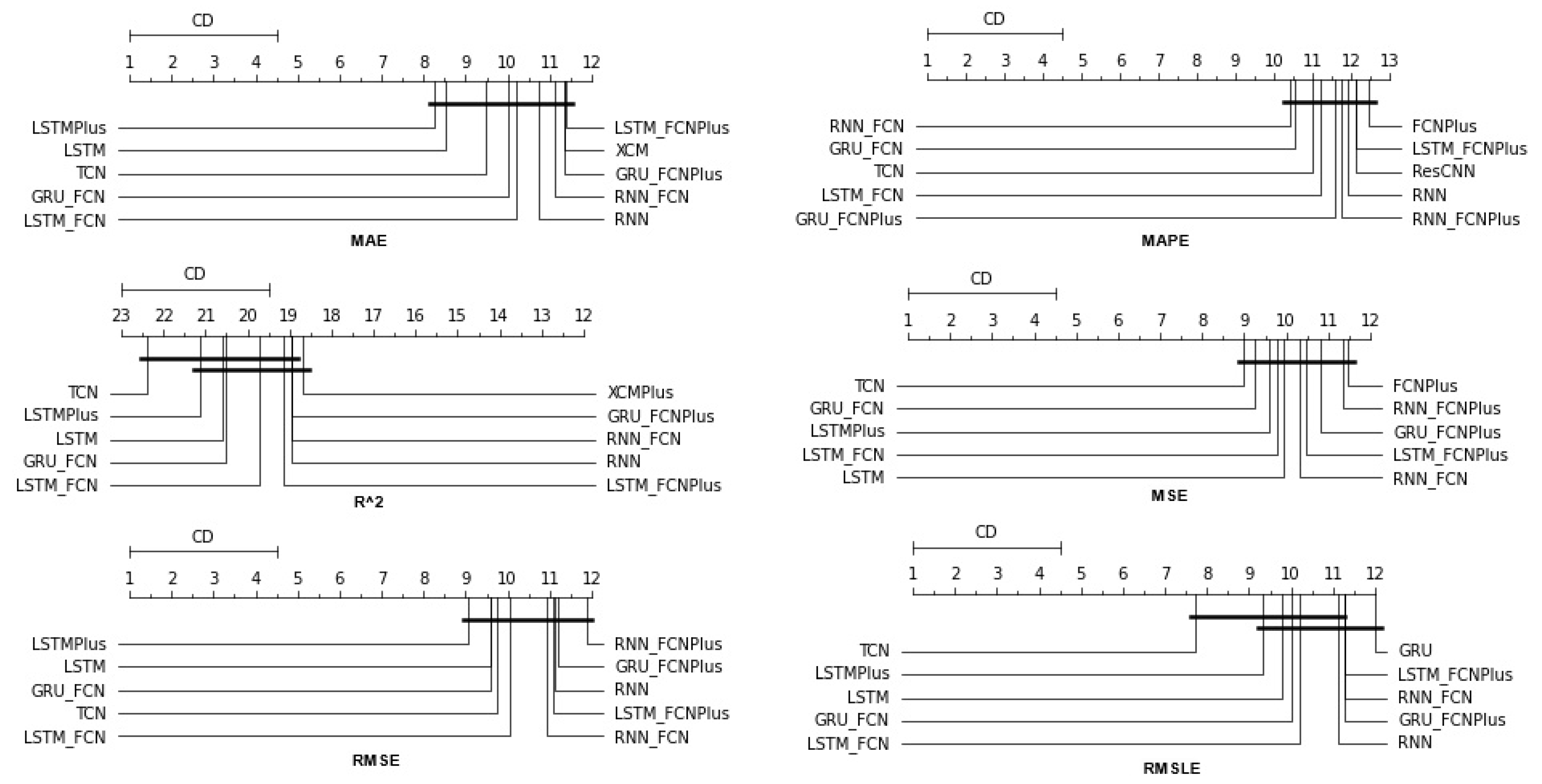
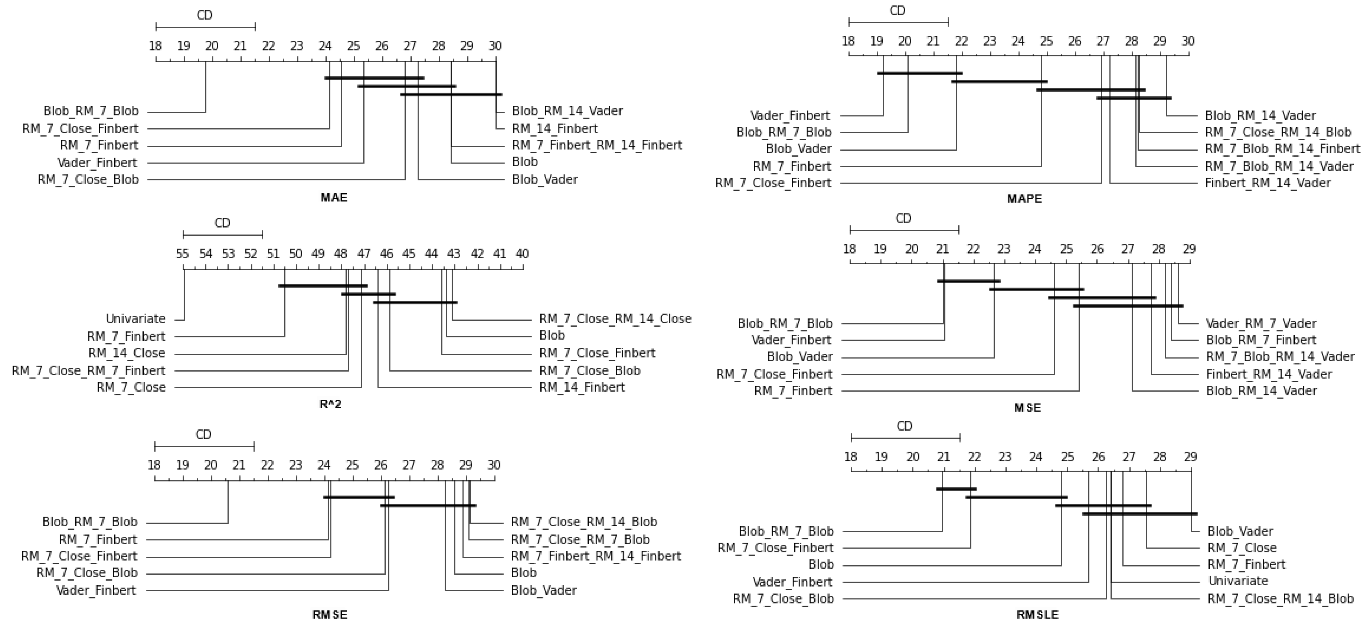
As has already been mentioned, during the procedure, for each of the stocks, the following strategy was followed: each of the thirty algorithms to be compared was “ran” 67 times, each time accepting as input one of the different feature setups. This was repeated three times, once for each of the three forecast time frames. In each of the above runs, the six metrics used in the evaluation of the results were calculated. The comparison of the algorithms was performed by using Friedman’s statistical tests in terms of feature setups for each of the time shifts. Thus, given setups and stocks, the ranking of the methods per evaluation metric was extracted according to the use of the Friedman test [88]. Therefore, regarding this case study, a total of 67 × 6 × 3 = 1206 statistical tests were executed. In a similar way, the Friedman rankings of input feature setups were estimated in terms of metrics and time shifts, given the various algorithms and stocks. Here, a total of 30 × 6 × 3 = 540 statistical tests were performed. An additional abstraction of the results was derived as follows: For each of the 30 methods, the average rank achieved by each method in terms of feature setups and shares was calculated. So, for each metric and each of the three time frames, a more comprehensive display of the information was obtained based on the average value of the different setups. In an identical way, in the case of checking the effectiveness of features, the average value of the 30 algorithms for each of the 67 different input setups was calculated in each case. In both cases, the ranking was calculated based on the positions produced by the Friedman test, while at the same time, with the Nemenyi post hoc test [89] that followed, every schema was checked pair-wise for significant differences. The results of the Nemenyi post hoc tests are shown in the corresponding Critical Difference diagrams (CD-diagrams), in which methods that are not significantly different are joined by black horizontal lines. Two methods are considered not significantly different when the difference between their mean ranks is less than the CD value.
Next, organized in both cases based on time frames, the results concerning the comparison of the forecast algorithms are presented, which are followed by those regarding the feature setups.
4.1. Method Comparison
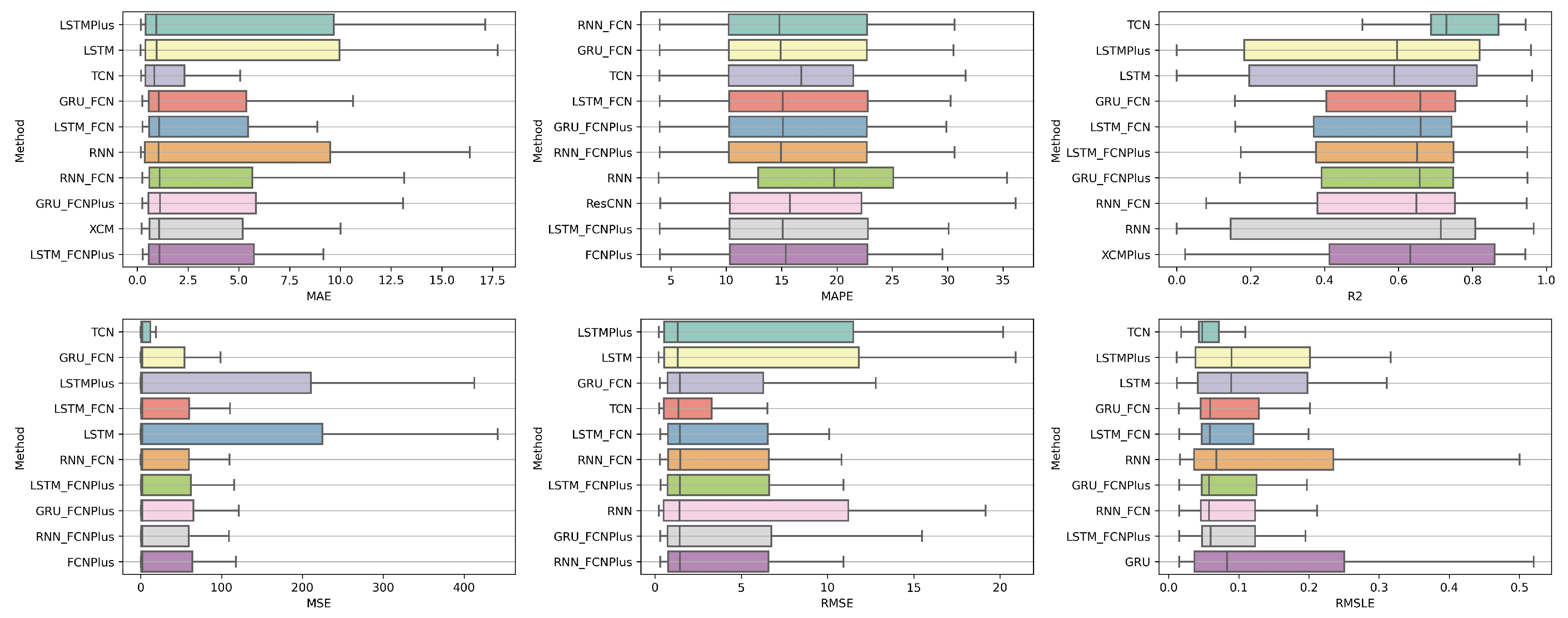
The presentation begins with results concerning the investigation of methods. The results are presented per forecast time shift. In each case, the Friedman Ranking results for all six metrics are listed. To save space, only methods that occupy the top ten positions of the ranking are listed. Full tables are available at: shorturl.at/FTU06 (accessed on 15 January 2023). The CD diagrams follow. There, we can visually observe which of the methods exhibit similar behavior and which differ significantly. Finally, box plots of results per metric are presented, again for the best 10 methods. The box plots present in a graphical and concise manner information concerning the distribution of the aforementioned data, that is, in our case, the average values of the sentiment setups per algorithm for all stocks. In particular, one can derive information about the maximum and minimum value of the data, the median, as well as the 1st and 3rd quartile values isolated by 25% and 75% of the observations, respectively.
4.1.1. Time Shift 1
With respect to the one-day forecasts, Table A1 lists the Friedman Ranking results for the top 10 scoring methods per metric. Although there is no single method that dominates all metrics and significant reorderings are also observed in the table positions, the TCN method achieves the best ranking in three out of six metrics (MAPE, R2, and RMSLE) and is always in the top four. Furthermore, from the box plots, it is evident that TCN has by far the smallest range of values.
Apart from this, in all metrics, GRU_FCN is always in the top five. It is also observed that LSTM_FCN and LSTMPlus behave equally well. The latter shows a drop in the MAPE metric, but in all other cases, it is in the top three, while in two metricsm it ranks first. It should also be noted that the LSTMPlus method ranks first in two metrics, namely MAE and RMSE. In terms of R and RMSLE, it occupies the second position of the ranking, while regarding MSE, LSTMPlus ranks third. However, at the same time, according to MAPE, the method is not even in the top ten. Thus, as will be seen in the following, TCN is the consistent choice.
4.1.2. Time Shift 7
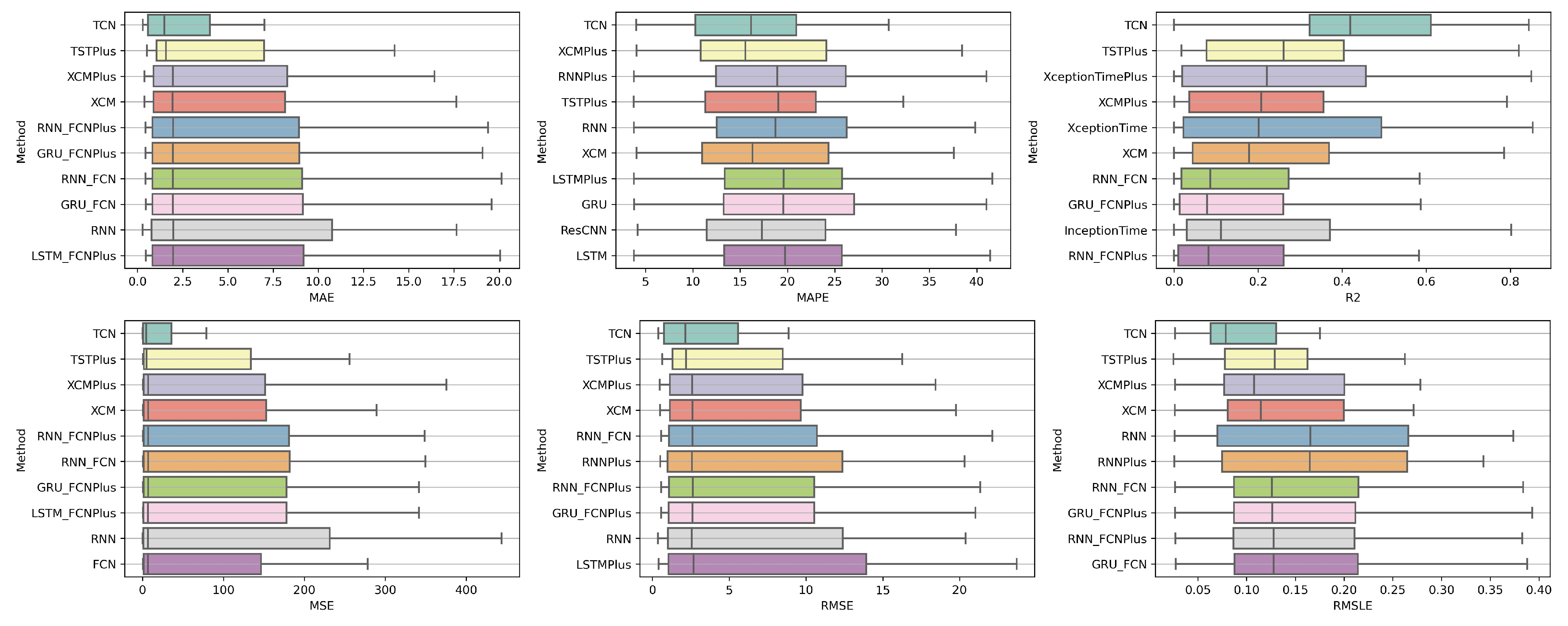
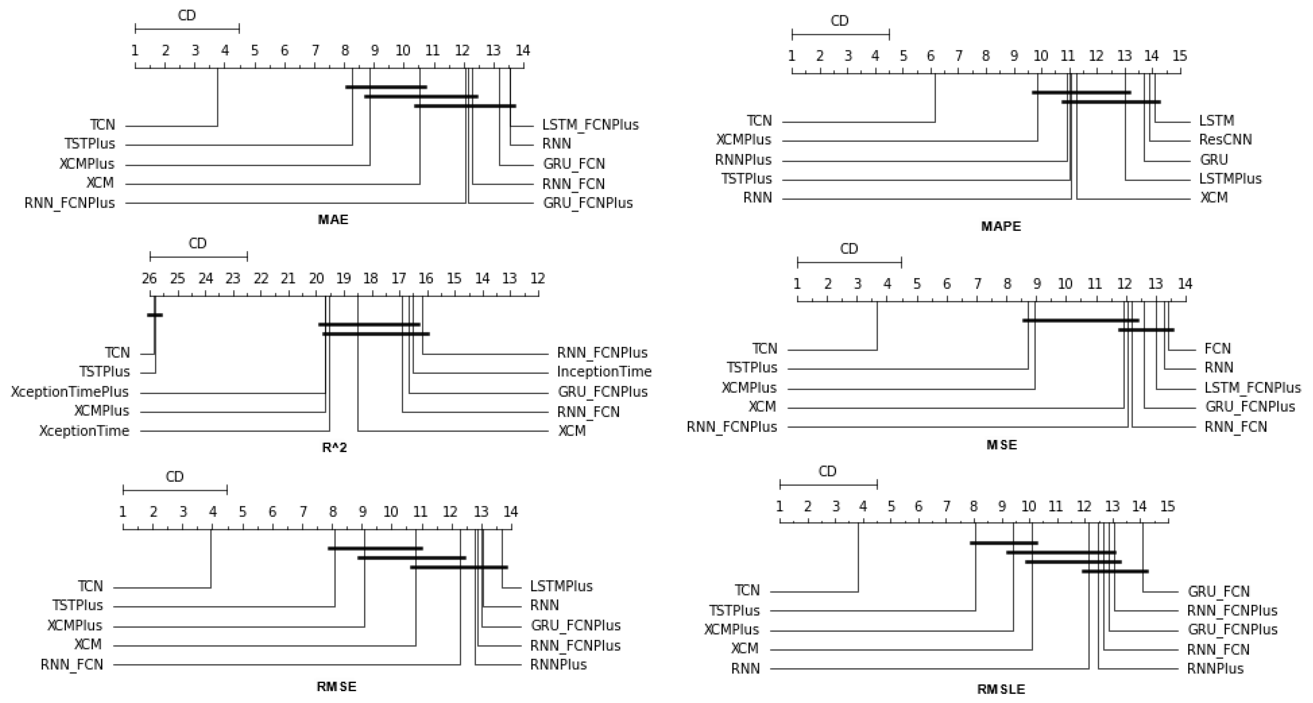
At the one-week forecast time frame, the algorithms that occupy the top positions in the ranking produced by the statistical control appear to have stabilized. The corresponding ranking produced by the Friedman statistical test regarding the ten best methods with respect to the six metrics is presented in Table A2. In all metrics, the TCN method ranks first. From the CD diagrams, it can be seen that in all metrics—except for R2—this superiority is also validated by the fact that this method differs significantly from the others. Box plots show the method also having the smallest range around the median. Figure 5 and Figure 6 contain the relevant results in the form of box plots and CD-diagrams.
Other methods that clearly show some dominance over the rest in terms of given performance ratings are, on the one hand, TSTPlus, which ranks second in all metrics except MAPE, and, on the other hand, XCMPlus and XCM, which are mostly found in the top five. In general, the same methods can be found in similar positions in all metrics, with minor rank variations. In addition, the statistical correlations between the methods are shown in the CD diagram plots.
4.1.3. Time Shift 14
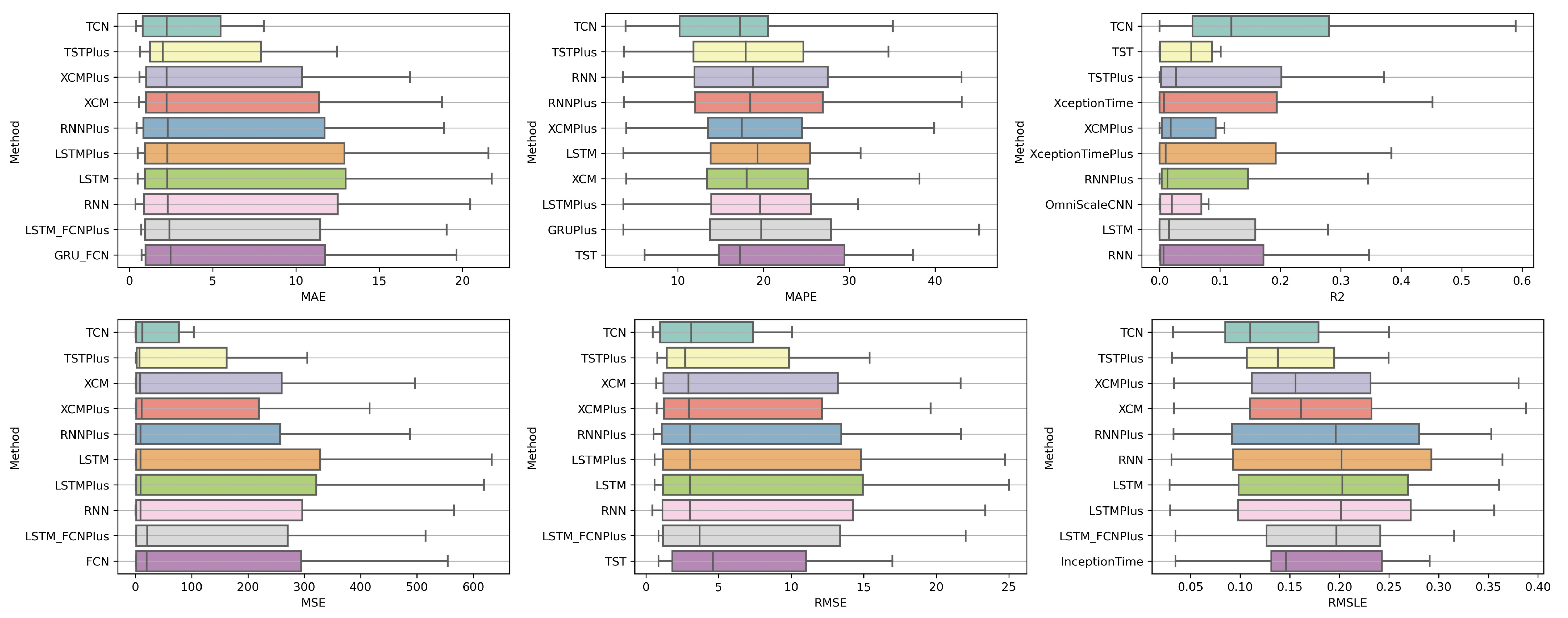
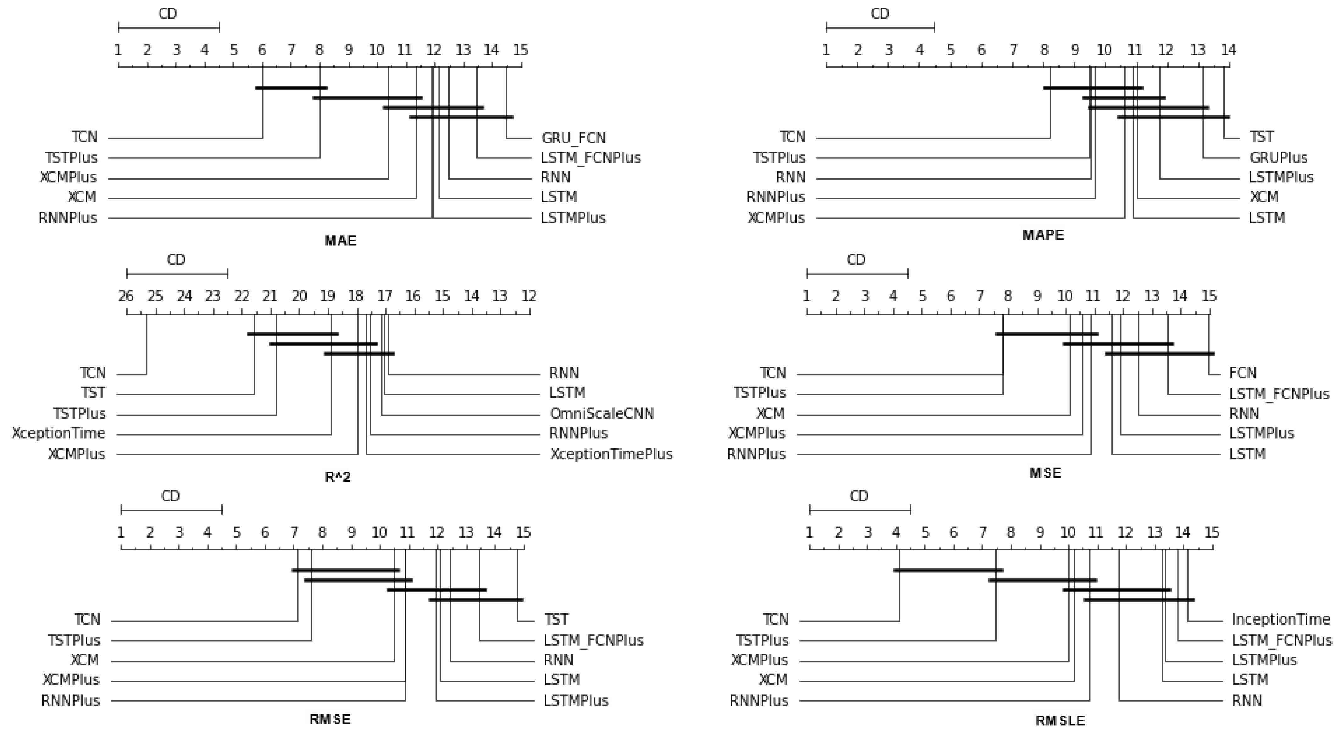
In the forecast results with a two-week shift, a relative agreement can be seen in the top-ranking algorithms with those of the one-week frames. The ranking produced by the Friedman statistical test for the ten best methods with respect to the six metrics is presented in Table A3.
Once more, TCN ranks first in all metrics. TSTPlus again ranks second in all metrics except for R2, where it ranks third. In almost all cases, XCMPlus and RNNPlus appear in the top five. Likewise, as in the previous time shift, there is a relative agreement in the methods appearing in the corresponding positions regarding all metrics. Moreover, according to the above, an argument regarding the general superiority of the TCN method in this particular scenario is easily obtained. An obvious predominance of the TCN method is established. The corresponding CD diagrams and box plots for the 10 best performing algorithms are seen in Figure 7 and Figure 8.
4.2. Feature Setup Comparison
Now, we are moving on to the findings of the second case study, which concern, on the one hand, the investigation of whether the use of sentiment analysis contributes to the improvement of the extracted predictions and, on the other hand, the identification of specific feature setups whose use improves the model’s predictive ability.
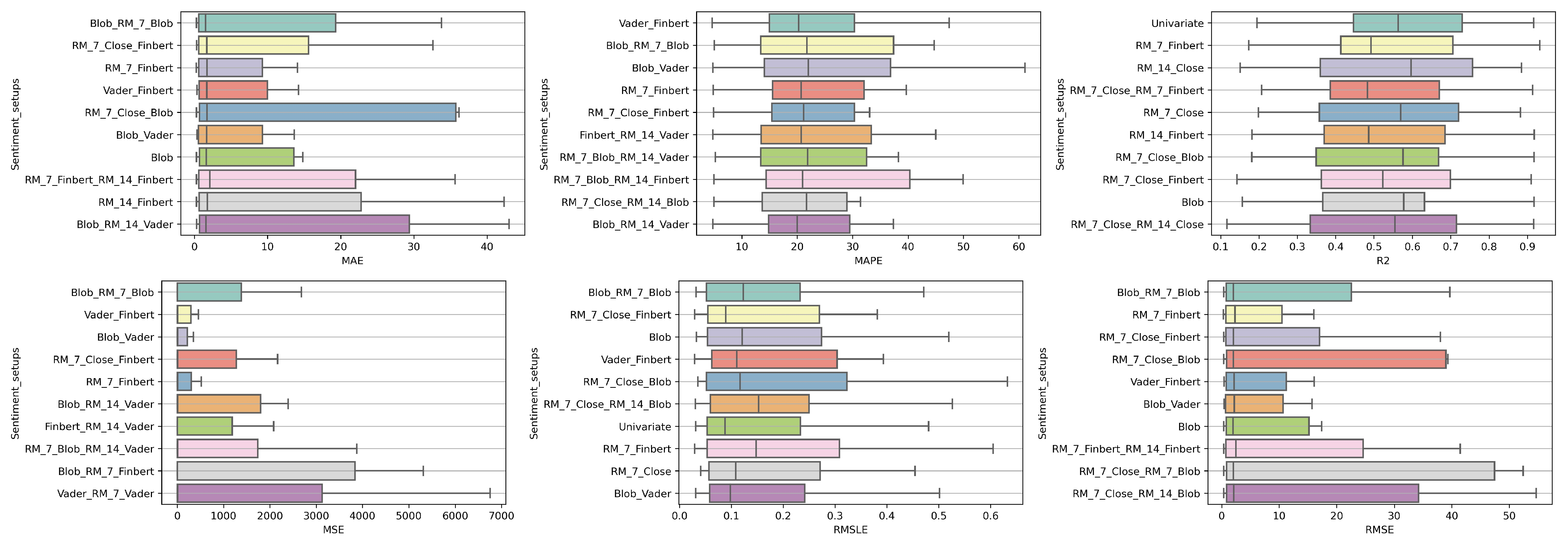
Again, the results of the experimental procedure will be presented separately for the three forecast time frames. Likewise, due to the volume of results, only the 10 most promising feature setups will be listed. These were again derived based on the Friedman classification of the averages calculated for each of them, taking into account the predictions in the use of the 30 forecast methods used. The full rankings of all 67 setups can be found at shorturl.at/alqwx (accessed on 13 December 2022). For the presentation below, again, the corresponding CD diagrams and box plots were used.
4.2.1. Time Shift 1
Starting with the results concerning one-day depth forecasting, one notices that the univariate version, in which the forecasts are based only on the stock price of the previous days, ranks first only in the case of the R metric. In fact, in three metrics, the univariate version is not even in the top twenty of the ranking (See Figure 9 and Figure 10).
Another interesting observation would be that even though there are rerankings of the sentiment setups in terms of their performance on the six metrics, the Blob_RM_7_Blob setup—that is, the setup incorporating Blob and Rolling Mean 7 Blob along with the closing values time series—although it does not score well in the ranking regarding R, it is, on the one hand, at the top ranking in four metrics, that is, MAE, MSE, RMSE, RMSLE, and, on the other hand, second in MAPE. Moreover, from the results, it becomes evident that an argument in favor of using sentiment analysis in multivariate time series layouts, even in the case where the forecasts concern one-day depth, is, at least, relevant. At the same time, using smoothed versions of both the sentiment time series and those containing the closing stock price values appears to be beneficial in general.
4.2.2. Time Shift 7
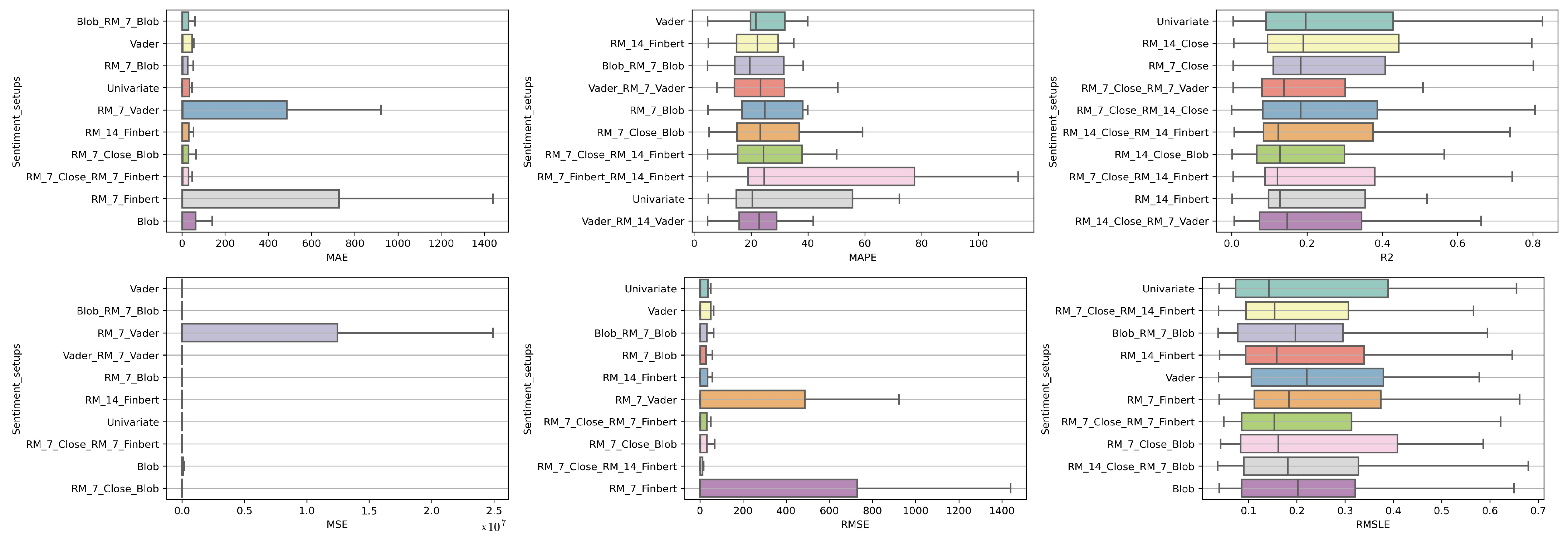
Regarding the time frame of one week, one can notice that the use of the univariate version is marginally ranked first in three metrics, namely, the R, RMSE and RMSLE, while in two metrics, the Vader sentiment setup appears to be superior, actually being, at the same time, in second place regarding the MAPE and RMSE metrics and fifth regarding the RMSLE (Figure 11 and Figure 12).
It is also notable that Blob_RM_7_Blob, which appeared to perform particularly well during the one-day shift, remains in the top three rankings in five of the six metrics. More generally, once again, one notices that there are rearrangements, especially in the central positions of the table. However, given the small differences in performance between the different setups, this should not be considered unreasonable. Overall, the picture still points in favor of using multivariate inputs containing sentiment data.
4.2.3. Time Shift 14
Finally, regarding the two-week time frame, a first observation is that in relation to the R, a feature setup that does not contain sentiment data dominates. This pattern is also present in the previous time shifts (See Figure 13 and Figure 14).
In addition, although there are metrics in which the univariate version is in the top ten, in these cases, the difference in its performance with those in the first positions is quite significant. This is easily seen from the CD diagrams: there are no connections with setups that appear in the top positions. At the seven-day time lag, it was observed that the univariate version prevailed in three cases. However, as one examines the 14-day time shift, one notices that the superiority of methods that use sentiment data is reinforced.
At the same time, combinations containing the closing price appear in the first positions of the table more often than in the previous two setups. Furthermore, it is observed that the setup that dominates four of the six metrics is RM_7_Close_Blob. These metrics are MAE, MAPE, MSE, and RMSE. The RM_7_Close_Blob feature setup is the one that incorporates both a smoothed version of the closing values as well as sentiment scores. Thus, the use of weighted averages in the original time series along with the incorporation of sentiment scores is mostly shown to be optimal regardless of the individual choice of a specific layout. Methodologically, the utilization of both has an improving effect.
5. Conclusions
Some general conclusions drawn from the whole experimental procedure will now be addressed. The discussion will follow the binary separation of the preceding case studies.
5.1. Methods
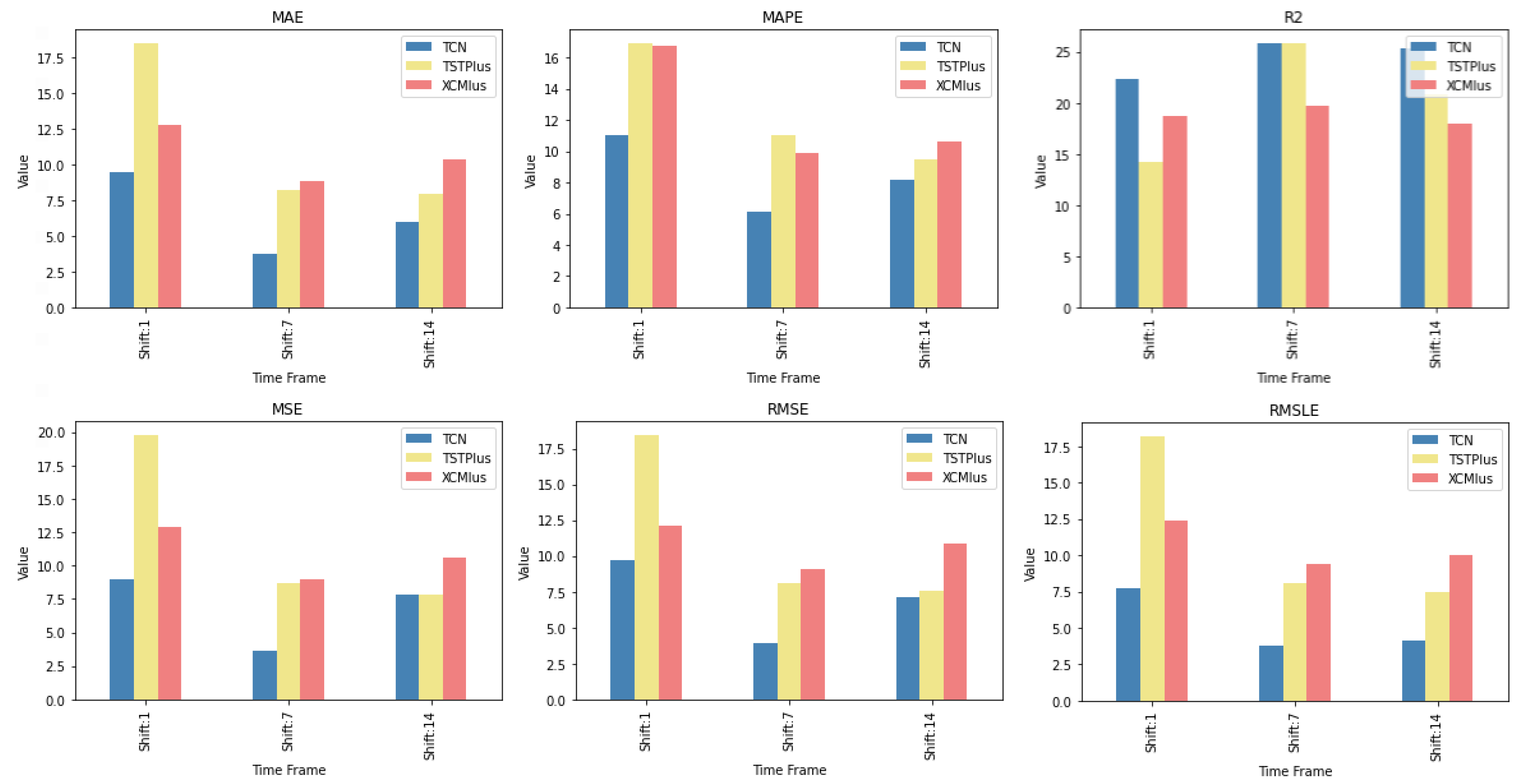
The first case study of the paper consisted of a comparison of 30 methods for time series forecasting. Within the above-discussed experimental context, the extracted results are such as to safely allow a conclusion regarding the superiority of the TCN method over the rest. This is the case because, in the vast majority of comparisons, it excels, being, for the most part, at the top of the Friedman ranking. In particular, the only cases where it does not outperform all the rest are found in the single-day time frame predictions. In fact, from the CD diagrams, one can extract the additional fact that in many cases, the superiority of the aforementioned method is marked by a significant difference. Furthermore, in addition to the TCN method, other methods whose predictive capacities can be considered significant were identified. TSTPlus is one of them, as it produces significant results, particularly over longer time horizons. XCMPlus is another.
In Figure 15, one can see the relative rankings of these three methods per time shift. The values in Figure 15 correspond to the values of Table A1, Table A2 and Table A3. Regarding the one-day forecast window, LSTMPlus is an additional option, as is the combination of GRU and FCN. However, an additional point to note here is that the individual method differences are less clear in their significance. On the contrary, there can also be conclusions regarding methods whose behavior was not evaluated, on average, as satisfactory. In particular, specific methods that are always ranked last in all scenarios were identified. Specifically, TSiTPlus ranks last in all three scenarios across all metrics. In addition to this, there are methods, such as Transformer Model, XceptionTime, and XceptionTimePlus, which are always at the bottom of the table in the vast majority of cases. In conclusion, given the limitations and further prerequisites developed throughout this paper, TCN can be easily recommended.
5.2. Feature and Sentiment Setups
In relation to the second case study, the consideration of the results also points in some important directions. Of these, the main conclusion drawn seems to be that the use of information derived from both smoothed versions of the initial time series and sentiment analysis shows, in most cases, to have a beneficial effect on the derived forecasts. Not using sentiments in the feature setup of the inputs dominates the rest only in a small number of cases, and, as confirmed by the CD diagrams, only in two of them is this difference significant.
Moreover, the answer to whether the use of sentiment setups specifically leads to the extraction of more accurate forecasts, as evidenced by the individual layouts of the weighted results, seems to be that, in general, sentiment analysis improves forecasts. Of course, it is also reasonable to investigate whether there is a specific sentiment setup that outperforms the rest. This would also lead to an assessment of the performance of the three sentiment analysis methods used. However, the answer to this question needs further investigation. However, even with the possibility of further inquiries within the framework of the experimental setup presented here, it is still not certain that firm conclusions will be drawn. Here, while such setups can be found for each time horizon, there is not one that dominates all three.
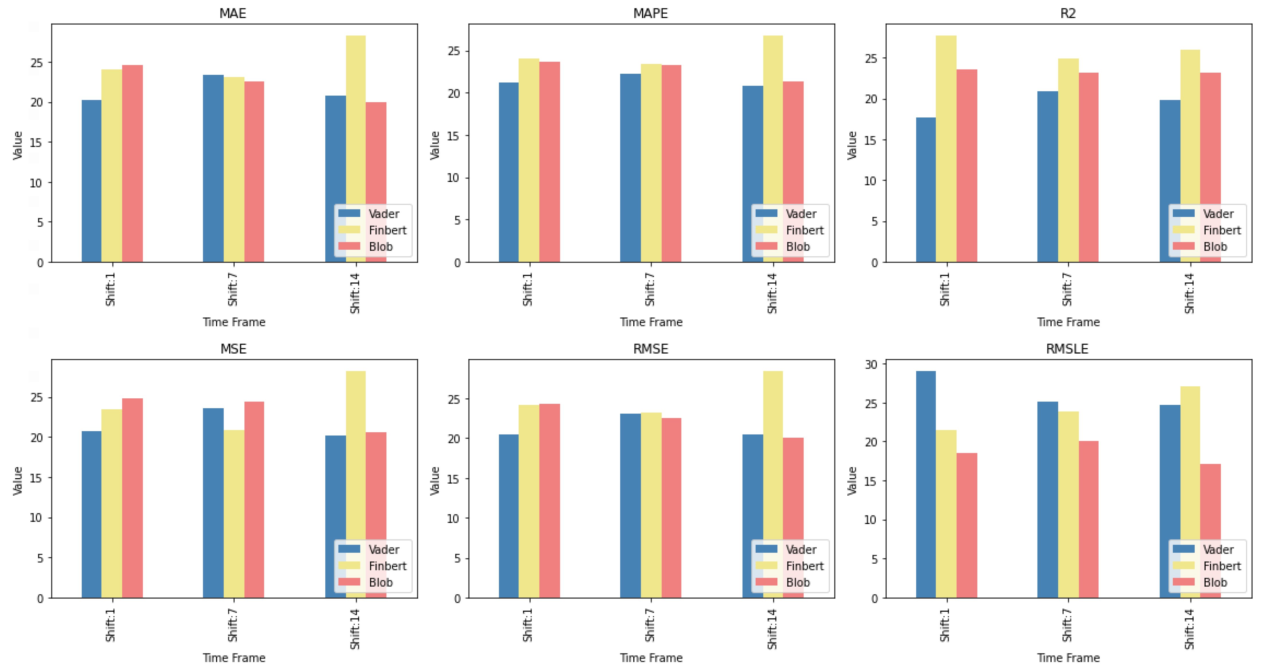
In order, however, to illustrate a relative ranking of the three sentiment analysis methodologies used, regardless of the particular variation involved, an additional table was created. All variations of each method were placed under a corresponding class. The Friedman-aligned ranks [90] were then calculated. Hence, in order to draw a clearer picture of the way the three employed approaches to sentiment analysis performed, three sentiment classes were formed, one matching each of the previously described sentiment analysis methods. The arithmetic mean of all the sentiment setups that solely contain different variations of a particular sentiment analysis algorithm, that is, only one of the three incorporated, is used to represent the corresponding class concerning each metric. In other words, each class represents a sentiment analysis method, and each class corresponds to six sentiment setups that contain variations exclusively of the technique in question. Specifically, a representative value of a class, as it pertains to a particular method, is formed by the following setups: method, RM7method, RM14method, method + RM7method, method + RM14method, and RM7method + RM14method. The sum is then divided by six, which is apparently the number of setups, and this result is the output value to be depicted. This way, setups produced either by combining the various sentiment analysis methods or by using the target variable in variants containing rolling means are excluded in order to compare only the relative performances of the three individual techniques and their variations.
Figure 16 illustrates these relative rankings of the three sentiment analysis methods per time shift. One can observe the relative performances in terms of individual wins with respect to each metric and time shift: the Blob and Vader classes top the ranking seven times each, while the Finbert class only has four wins. Again, a conclusion in terms of an obvious generality regarding a specific algorithm does not appear. Nevertheless, the identification of groups of such setups, even at the level of a specific time frame, can be particularly useful, with the methodology for the selection of individual setups needing more investigation.
Author Contributions
Conceptualization, C.M.L. and S.K.; methodology, C.M.L.; software, C.M.L.; validation, C.M.L., A.K. and S.K.; formal analysis, C.M.L. and A.K.; investigation, C.M.L. and A.K.; resources, S.K.; data curation, A.K.; writing—original draft preparation, C.M.L. and A.K.; writing—review and editing, C.M.L.; visualization, A.K.; supervision, S.K. All authors have read and agreed to the published version of the manuscript.
Funding
This research received no external funding.
Institutional Review Board Statement
Not applicable.
Data Availability Statement
URLs of the full Friedman Ranking results. (i) Methods rankings: shorturl.at/FTU06 (accessed on 15 January 2023). (ii) Feature setup rankings: shorturl.at/alqwx (accessed on 15 January 2023).
Conflicts of Interest
The authors declare no conflict of interest.
Appendix A
Table A1.
Friedman results: Algorithms—Shift 1.
| MAE | MAPE | R | ||||
|---|---|---|---|---|---|---|
| Method | Friedman Score | Method | Friedman Score | Method | Friedman Score | |
| 1st | LSTMPlus | 8.266667 | RNN_FCN | 10.4 | TCN | 22.4 |
| 2nd | LSTM | 8.533333 | GRU_FCN | 10.53333 | LSTMPlus | 21.13333 |
| 3rd | TCN | 9.466667 | TCN | 11 | LSTM | 20.6 |
| 4th | GRU_FCN | 10 | LSTM_FCN | 11.2 | GRU_FCN | 20.53333 |
| 5th | LSTM_FCN | 10.2 | GRU_FCNPlus | 11.6 | LSTM_FCN | 19.73333 |
| 6th | RNN | 10.73333 | RNN_FCNPlus | 11.73333 | LSTM_FCNPlus | 19.13333 |
| 7th | RNN_FCN | 11.13333 | RNN | 11.93333 | GRU_FCNPlus | 18.93333 |
| 8th | GRU_FCNPlus | 11.33333 | ResCNN | 12.13333 | RNN_FCN | 18.93333 |
| 9th | XCM | 11.33333 | LSTM_FCNPlus | 12.13333 | RNN | 18.93333 |
| 10th | LSTM_FCNPlus | 11.4 | FCNPlus | 12.46667 | XCMPlus | 18.66667 |
| MSE | RMSE | RMSLE | ||||
| Method | Friedman Score | Method | Friedman Score | Method | Friedman Score | |
| 1st | TCN | 9 | LSTMPlus | 9.066667 | TCN | 7.733333 |
| 2nd | GRU_FCN | 9.266667 | LSTM | 9.6 | LSTMPlus | 9.333333 |
| 3rd | LSTMPlus | 9.6 | GRU_FCN | 9.6 | LSTM | 9.8 |
| 4th | LSTM_FCN | 9.8 | TCN | 9.733333 | GRU_FCN | 10 |
| 5th | LSTM | 9.933333 | LSTM_FCN | 10.06667 | LSTM_FCN | 10.2 |
| 6th | RNN_FCN | 10.33333 | RNN_FCN | 10.93333 | RNN | 11.13333 |
| 7th | LSTM_FCNPlus | 10.46667 | LSTM_FCNPlus | 11.06667 | GRU_FCNPlus | 11.26667 |
| 8th | GRU_FCNPlus | 10.8 | RNN | 11.13333 | RNN_FCN | 11.26667 |
| 9th | RNN_FCNPlus | 11.33333 | GRU_FCNPlus | 11.2 | LSTM_FCNPlus | 11.26667 |
| 10th | FCNPlus | 11.46667 | RNN_FCNPlus | 11.86667 | GRU | 12 |
Table A2.
Friedman results: Algorithms—Shift 7.
| MAE | MAPE | R | ||||
|---|---|---|---|---|---|---|
| Method | Friedman Score | Method | Friedman Score | Method | Friedman Score | |
| 1st | TCN | 3.733333 | TCN | 6.133333 | TCN | 25.86667 |
| 2nd | TSTPlus | 8.266667 | XCMPlus | 9.866667 | TSTPlus | 25.8 |
| 3rd | XCMPlus | 8.866667 | RNNPlus | 10.93333 | XceptionTimePlus | 19.7 |
| 4th | XCM | 10.53333 | TSTPlus | 11 | XCMPlus | 19.66667 |
| 5th | RNN_FCNPlus | 12.06667 | RNN | 11.06667 | XceptionTime | 19.53333 |
| 6th | GRU_FCNPlus | 12.13333 | XCM | 11.26667 | XCM | 18.53333 |
| 7th | RNN_FCN | 12.26667 | LSTMPlus | 13 | RNN_FCN | 16.9 |
| 8th | GRU_FCN | 13.2 | GRU | 13.66667 | GRU_FCNPlus | 16.66667 |
| 9th | RNN | 13.53333 | ResCNN | 13.86667 | InceptionTime | 16.5 |
| 10th | LSTM_FCNPlus | 13.53333 | LSTM | 14.06667 | RNN_FCNPlus | 16.16667 |
| MSE | RMSE | RMSLE | ||||
| Method | Friedman Score | Method | Friedman Score | Method | Friedman Score | |
| 1st | TCN | 3.666666667 | TCN | 3.933333333 | TCN | 3.8 |
| 2nd | TSTPlus | 8.733333333 | TSTPlus | 8.066666667 | TSTPlus | 8.066666667 |
| 3rd | XCMPlus | 8.933333333 | XCMPlus | 9.066666667 | XCMPlus | 9.4 |
| 4th | XCM | 11.93333333 | XCM | 10.8 | XCM | 10.06666667 |
| 5th | RNN_FCNPlus | 12.06666667 | RNN_FCN | 12.26666667 | RNN | 12.13333333 |
| 6th | RNN_FCN | 12.2 | RNNPlus | 12.8 | RNNPlus | 12.46666667 |
| 7th | GRU_FCNPlus | 12.6 | RNN_FCNPlus | 12.86666667 | RNN_FCN | 12.66666667 |
| 8th | LSTM_FCNPlus | 13 | GRU_FCNPlus | 13 | GRU_FCNPlus | 12.86666667 |
| 9th | RNN | 13.26666667 | RNN | 13.06666667 | RNN_FCNPlus | 13.06666667 |
| 10th | FCN | 13.4 | LSTMPlus | 13.66666667 | GRU_FCN | 14.06666667 |
Table A3.
TFriedman results: Algorithms—Shift 14.
| MAE | MAPE | R | ||||
|---|---|---|---|---|---|---|
| Method | Friedman Score | Method | Friedman Score | Method | Friedman Score | |
| 1st | TCN | 6 | TCN | 8.2 | TCN | 25.33333333 |
| 2nd | TSTPlus | 8 | TSTPlus | 9.466666667 | TST | 21.6 |
| 3rd | XCMPlus | 10.4 | RNN | 9.533333333 | TSTPlus | 20.8 |
| 4th | XCM | 11.33333333 | RNNPlus | 9.666666667 | XceptionTime | 18.9 |
| 5th | RNNPlus | 11.86666667 | XCMPlus | 10.6 | XCMPlus | 17.96666667 |
| 6th | LSTMPlus | 11.93333333 | LSTM | 10.86666667 | XceptionTimePlus | 17.7 |
| 7th | LSTM | 12.13333333 | XCM | 11 | RNNPlus | 17.53333333 |
| 8th | RNN | 12.46666667 | LSTMPlus | 11.73333333 | OmniScaleCNN | 17.13333333 |
| 9th | LSTM_FCNPlus | 13.46666667 | GRUPlus | 13.13333333 | LSTM | 17.03333333 |
| 10th | GRU_FCN | 14.46666667 | TST | 13.8 | RNN | 16.93333333 |
| MSE | RMSE | RMSLE | ||||
| Method | Friedman Score | Method | Friedman Score | Method | Friedman Score | |
| 1st | TCN | 7.8 | TCN | 7.133333333 | TCN | 4.133333333 |
| 2nd | TSTPlus | 7.8 | TSTPlus | 7.6 | TSTPlus | 7.466666667 |
| 3rd | XCM | 10.13333333 | XCM | 10.46666667 | XCMPlus | 10 |
| 4th | XCMPlus | 10.6 | XCMPlus | 10.86666667 | XCM | 10.2 |
| 5th | RNNPlus | 10.86666667 | RNNPlus | 10.86666667 | RNNPlus | 10.73333333 |
| 6th | LSTM | 11.6 | LSTMPlus | 11.93333333 | RNN | 11.73333333 |
| 7th | LSTMPlus | 11.86666667 | LSTM | 12.06666667 | LSTM | 13.26666667 |
| 8th | RNN | 12.53333333 | RNN | 12.4 | LSTMPlus | 13.33333333 |
| 9th | LSTM_FCNPlus | 13.53333333 | LSTM_FCNPlus | 13.46666667 | LSTM_FCNPlus | 13.8 |
| 10th | FCN | 14.93333333 | TST | 14.73333333 | InceptionTime | 14.13333333 |
Appendix B
Appendix B.1
Please use the abbreviation table below to read the corresponding results of the Friedman Ranks.
Table A4.
Feature Setups and Abbreviations.
| No. | Abbreviation | Feature Setup |
|---|---|---|
| 1 | U | Univariate |
| 2 | B | Blob |
| 3 | V | Vader |
| 4 | F | Finbert |
| 5 | RM7C | Rolling Mean 7 Closing Value |
| 6 | RM14C | Rolling Mean 14 Closing Value |
| 7 | RM7B | Rolling Mean 7 Blob |
| 8 | RM14B | Rolling Mean 14 Blob |
| 9 | RM7V | Rolling Mean 7 Vader |
| 10 | RM14V | Rolling Mean 14 Vader |
| 11 | RM7F | Rolling Mean 7 Finbert |
| 12 | RM14F | Rolling Mean 14 Finbert |
Appendix B.2
Table A5.
Friedman results: feature setups—Shift 1.
| MAE | MAPE | R | ||||
|---|---|---|---|---|---|---|
| Feature Setup | Friedman Score | Feature Setup | Friedman Score | Feature Setup | Friedman Score | |
| 1st | B_RM7B | 19.73333 | V_F | 19.2 | U | 54.93333 |
| 2nd | RM7C_F | 24.13333 | B_RM7B | 20.06667 | RM7F | 50.53333 |
| 3rd | RM7F | 24.53333 | B_V | 21.8 | RM14C | 47.8 |
| 4th | V_F | 25.33333 | RM7F | 24.8 | RM7C_RM7F | 47.73333 |
| 5th | RM7C_B | 26.8 | RM7C_F | 26.93333 | RM7C | 47.13333 |
| 6th | B_V | 27.26667 | F_RM14V | 27.2 | RM14F | 46.4 |
| 7th | B | 28.4 | RM7B_RM14V | 28.13333 | RM7C_B | 45.86667 |
| 8th | RM7F_RM14F | 28.4 | RM7B_RM14F | 28.2 | RM7C_F | 43.6 |
| 9th | RM14F | 30 | RM7C_RM14B | 28.26667 | B | 43.4 |
| 10th | B_RM14V | 30 | B_RM14V | 29.2 | RM7C_RM14C | 43.13333 |
| MSE | RMSE | RMSLE | ||||
| Feature Setup | Friedman Score | Feature Setup | Friedman Score | Feature Setup | Friedman Score | |
| 1st | B_RM7B | 21 | B_RM7B | 20.6 | B_RM7B | 20.93333 |
| 2nd | V_F | 21.06667 | RM7F | 24.13333 | RM7C_F | 21.86667 |
| 3rd | B_V | 22.66667 | RM7C_F | 24.2 | B | 24.8 |
| 4th | RM7C_F | 24.6 | RM7C_B | 26.13333 | V_F | 25.66667 |
| 5th | RM7F | 25.4 | V_F | 26.26667 | RM7C_B | 26.26667 |
| 6th | B_RM14V | 27.13333 | B_V | 28.26667 | RM7C_RM14B | 26.4 |
| 7th | F_RM14V | 27.73333 | B | 28.6 | U | 26.4 |
| 8th | RM7B_RM14V | 28.2 | RM7F_RM14F | 28.86667 | RM7F | 26.8 |
| 9th | B_RM7F | 28.4 | RM7C_RM7B | 29.06667 | RM7C | 27.53333 |
| 10th | V_RM7V | 28.6 | RM7C_RM14B | 29.13333 | B_V | 29 |
Table A6.
Friedman results: feature setups—Shift 7.
| MAE | MAPE | R | ||||
|---|---|---|---|---|---|---|
| Feature Setup | Friedman Score | Feature Setup | Friedman Score | Feature Setup | Friedman Score | |
| 1st | B_RM7B | 21.53333 | V | 22.33333 | U | 55.06667 |
| 2nd | V | 22.8 | RM14F | 24.8 | RM14C | 54.93333 |
| 3rd | RM7B | 24.46667 | B_RM7B | 25.2 | RM7C | 54 |
| 4th | U | 24.86667 | V_RM7V | 25.93333 | RM7C_RM7V | 49.33333 |
| 5th | RM7V | 25.33333 | RM7B | 26.33333 | RM7C_RM14C | 47.23333 |
| 6th | RM14F | 25.53333 | RM7C_B | 26.66667 | RM14C_RM14F | 45.46667 |
| 7th | RM7C_B | 25.86667 | RM7C_RM14F | 26.8 | RM14C_B | 45.33333 |
| 8th | RM7C_RM7F | 26.66667 | RM7F_RM14F | 27.53333 | RM7C_RM14F | 45.26667 |
| 9th | RM7F | 26.86667 | U | 27.73333 | RM14F | 45.13333 |
| 10th | B | 27.13333 | V_RM14V | 27.93333 | RM14C_RM7V | 44.93333 |
| MSE | RMSE | RMSLE | ||||
| Feature Setup | Friedman Score | Feature Setup | Friedman Score | Feature Setup | Friedman Score | |
| 1st | V | 21.93333 | U | 22.73333 | U | 17.6 |
| 2nd | B_RM7B | 23.13333 | V | 23.13333 | RM7C_RM14F | 21.13333 |
| 3rd | RM7V | 24 | B_RM7B | 23.66667 | B_RM7B | 22.53333 |
| 4th | V_RM7V | 24.8 | RM7B | 24.46667 | RM14F | 22.73333 |
| 5th | RM7B | 25.53333 | RM14F | 24.93333 | V | 23.2 |
| 6th | RM14F | 26.73333 | RM7V | 25.4 | RM7F | 24.46667 |
| 7th | U | 27.2 | RM7C_RM7F | 25.8 | RM7C_RM7F | 25.73333 |
| 8th | RM7C_RM7F | 27.73333 | RM7C_B | 25.93333 | RM7C_B | 26.4 |
| 9th | B | 27.86667 | RM7C_RM14F | 26.6 | RM14C_RM7B | 26.73333 |
| 10th | RM7C_B | 27.93333 | RM7F | 27.2 | B | 26.86667 |
Table A7.
Friedman results: feature setups—Shift 14.
| MAE | MAPE | R | ||||
|---|---|---|---|---|---|---|
| Feature Setup | Friedman Score | Feature Setup | Friedman Score | Feature Setup | Friedman Score | |
| 1st | RM7C_B | 17.46667 | RM7C_B | 18.53333 | RM14C | 50.5 |
| 2nd | RM7C_V | 21.53333 | RM14C_B | 22.2 | RM7C | 48.9 |
| 3rd | RM14C_B | 22.26667 | RM7C_V | 22.93333 | U | 48.76667 |
| 4th | RM7C | 22.26667 | RM7F_RM14F | 23.73333 | RM14C_RM7F | 48.16667 |
| 5th | U | 23.73333 | B_RM7V | 24.2 | RM14C_RM7B | 46.83333 |
| 6th | B_RM7V | 23.8 | V | 25.6 | RM7C_RM7B | 46.06667 |
| 7th | V | 24.46667 | RM7C_F | 26.33333 | RM7C_RM7F | 45.76667 |
| 8th | RM7C_F | 24.86667 | V_RM14F | 27.4 | RM7C_RM14C | 45.56667 |
| 9th | RM7B | 25.86667 | RM7C | 27.66667 | RM7F | 43.83333 |
| 10th | RM14B | 27.33333 | RM7B | 28.13333 | RM14C_F | 43.36667 |
| MSE | RMSE | RMSLE | ||||
| Feature Setup | Friedman Score | Feature Setup | Friedman Score | Feature Setup | Friedman Score | |
| 1st | RM7C_B | 18.26667 | RM7C_B | 15.86667 | RM7C | 13.8 |
| 2nd | RM7C_V | 21.26667 | RM7C | 20.33333 | RM7C_B | 16 |
| 3rd | B_RM7V | 21.6 | RM14C_B | 21.26667 | RM14C_B | 21.06667 |
| 4th | RM14C_B | 23.86667 | RM7C_V | 21.4 | U | 22.33333 |
| 5th | V | 25.06667 | U | 22.8 | RM7C_F | 24.13333 |
| 6th | RM7B | 25.86667 | RM7C_F | 24 | RM14B | 24.33333 |
| 7th | RM7C | 26.2 | V | 24.06667 | B_RM7V | 25.06667 |
| 8th | RM7C_F | 26.26667 | B_RM7V | 24.46667 | RM7C_V | 26.06667 |
| 9th | RM7B_RM7F | 26.33333 | RM7B | 26 | V | 26.26667 |
| 10th | RM7B_RM7V | 26.66667 | RM7C_RM14C | 26.2 | RM7B | 26.46667 |
References
- Basak, S.; Kar, S.; Saha, S.; Khaidem, L.; Dey, S.R. Predicting the direction of stock market prices using tree-based classifiers. N. Am. J. Econ. Financ. 2019, 47, 552–567. [Google Scholar] [CrossRef]
- Ren, R.; Wu, D.D.; Liu, T. Forecasting Stock Market Movement Direction Using Sentiment Analysis and Support Vector Machine. IEEE Syst. J. 2019, 13, 760–770. [Google Scholar] [CrossRef]
- Huang, W.; Nakamori, Y.; Wang, S.Y. Forecasting stock market movement direction with support vector machine. Comput. Oper. Res. 2005, 32, 2513–2522. [Google Scholar] [CrossRef]
- Zhong, X.; Enke, D. Predicting the daily return direction of the stock market using hybrid machine learning algorithms. Financ. Innov. 2019, 5, 24. [Google Scholar] [CrossRef]
- Abraham, B.; Ledolter, J. (Eds.) Statistical Methods for Forecasting; Wiley Series in Probability and Statistics, John Wiley & Sons, Inc.: Hoboken, NJ, USA, 1983. [Google Scholar] [CrossRef]
- Armstrong, J.S.; Collopy, F.L. Integration of Statistical Methods and Judgment for Time Series Forecasting: Principles from Empirical Research. Forecast. Model. eJournal 1998, 269–293. [Google Scholar]
- Bontempi, G.; Ben Taieb, S.; Le Borgne, Y.A. Machine Learning Strategies for Time Series Forecasting; Springer: Berlin/Heidelberg, Germany, 2013; Volume 138. [Google Scholar] [CrossRef]
- Masini, R.P.; Medeiros, M.C.; Mendes, E.F. Machine learning advances for time series forecasting. J. Econ. Surv. 2021, 37, 76–111. [Google Scholar] [CrossRef]
- Cao, L.; Tay, F. Support vector machine with adaptive parameters in financial time series forecasting. IEEE Trans. Neural Netw. 2003, 14, 1506–1518. [Google Scholar] [CrossRef] [PubMed] [Green Version]
- Yang, A.; Li, W.; Yang, X. Short-term electricity load forecasting based on feature selection and Least Squares Support Vector Machines. Knowl.-Based Syst. 2019, 163, 159–173. [Google Scholar] [CrossRef]
- Sagheer, A.; Kotb, M. Time series forecasting of petroleum production using deep LSTM recurrent networks. Neurocomputing 2019, 323, 203–213. [Google Scholar] [CrossRef]
- Zhao, Z.; Chen, W.; Wu, X.; Chen, P.C.Y.; Liu, J. LSTM network: A deep learning approach for short-term traffic forecast. IET Intell. Transp. Syst. 2017, 11, 68–75. [Google Scholar]
- Graf, R.; Zhu, S.; Sivakumar, B. Forecasting river water temperature time series using a wavelet–neural network hybrid modelling approach. J. Hydrol. 2019, 578, 124115. [Google Scholar] [CrossRef]
- Kurumatani, K. Time series forecasting of agricultural product prices based on recurrent neural networks and its evaluation method. SN Appl. Sci. 2020, 2, 1434. [Google Scholar]
- Khairalla, M.A.E.; Ning, X.; Al-Jallad, N.T.; El-Faroug, M.O. Short-Term Forecasting for Energy Consumption through Stacking Heterogeneous Ensemble Learning Model. Energies 2018, 11, 1605. [Google Scholar] [CrossRef] [Green Version]
- Alkandari, M.; Ahmad, I. Solar power generation forecasting using ensemble approach based on deep learning and statistical methods. Appl. Comput. Inform. 2020. [Google Scholar] [CrossRef]
- Liapis, C.M.; Karanikola, A.; Kotsiantis, S.B. Energy Load Forecasting: Investigating Mid-Term Predictions with Ensemble Learners. In Proceedings of the AIAI, Crete, Greece, 17–20 June 2022. [Google Scholar]
- Liapis, C.M.; Karanikola, A.C.; Kotsiantis, S.B. An ensemble forecasting method using univariate time series COVID-19 data. In Proceedings of the 24th Pan-Hellenic Conference on Informatics, Athens, Greece, 20–22 November 2020. [Google Scholar]
- Liapis, C.M.; Karanikola, A.; Kotsiantis, S.B. A Multi-Method Survey on the Use of Sentiment Analysis in Multivariate Financial Time Series Forecasting. Entropy 2021, 23, 1603. [Google Scholar] [CrossRef] [PubMed]
- Siami-Namini, S.; Tavakoli, N.; Namin, A.S. A Comparison of ARIMA and LSTM in Forecasting Time Series. In Proceedings of the 2018 17th IEEE International Conference on Machine Learning and Applications (ICMLA), Orlando, FL, USA, 17–20 December 2018; pp. 1394–1401. [Google Scholar]
- Çıbıkdiken, A.; Karakoyun, E. Comparison of ARIMA Time Series Model and LSTM Deep Learning Algorithm for Bitcoin Price Forecasting. In Proceedings of the 13th multidisciplinary academic conference in Prague, Hamburg, Germany, 27–30 August 2018. [Google Scholar]
- Yamak, P.T.; Yujian, L.; Gadosey, P.K. A Comparison between ARIMA, LSTM, and GRU for Time Series Forecasting. In Proceedings of the ACAI, Sanya, China, 20–22 December 2019. [Google Scholar]
- Maleki, A.; Nasseri, S.; Aminabad, M.S.; Hadi, M. Comparison of ARIMA and NNAR Models for Forecasting Water Treatment Plant’s Influent Characteristics. KSCE J. Civ. Eng. 2018, 22, 3233–3245. [Google Scholar]
- Satrio, C.B.A.; Darmawan, W.; Nadia, B.U.; Hanafiah, N. Time series analysis and forecasting of coronavirus disease in Indonesia using ARIMA model and PROPHET. Procedia Comput. Sci. 2021, 179, 524–532. [Google Scholar]
- Paliari, I.; Karanikola, A.; Kotsiantis, S.B. A comparison of the optimized LSTM, XGBOOST and ARIMA in Time Series forecasting. In Proceedings of the 2021 12th International Conference on Information, Intelligence, Systems & Applications (IISA), Chania Crete, Greece, 12–14 July 2021; pp. 1–7. [Google Scholar]
- Zhang, Y.; Yang, H.L.; Cui, H.; Chen, Q. Comparison of the Ability of ARIMA, WNN and SVM Models for Drought Forecasting in the Sanjiang Plain, China. Nat. Resour. Res. 2019, 29, 1447–1464. [Google Scholar]
- Tealab, A. Time series forecasting using artificial neural networks methodologies: A systematic review. Future Comput. Inform. J. 2018, 3, 334–340. [Google Scholar] [CrossRef]
- Sezer, O.B.; Gudelek, M.U.; Ozbayoglu, A.M. Financial Time Series Forecasting with Deep Learning: A Systematic Literature Review: 2005–2019. arXiv 2020, arXiv:abs/1911.13288. [Google Scholar] [CrossRef] [Green Version]
- Lara-Benítez, P.; Carranza-García, M.; Santos, J.C.R. An Experimental Review on Deep Learning Architectures for Time Series Forecasting. Int. J. Neural Syst. 2021, 31, 2130001. [Google Scholar] [CrossRef] [PubMed]
- Karanikola, A.; Liapis, C.M.; Kotsiantis, S. A Comparison of Contemporary Methods on Univariate Time Series Forecasting. In Advances in Machine Learning/Deep Learning-Based Technologies: Selected Papers in Honour of Professor Nikolaos G. Bourbakis—Volume 2; Tsihrintzis, G.A., Virvou, M., Jain, L.C., Eds.; Springer International Publishing: Cham, Switzerland, 2022; pp. 143–168. [Google Scholar] [CrossRef]
- Wang, K.; Qi, X.; Liu, H. A comparison of day-ahead photovoltaic power forecasting models based on deep learning neural network. Appl. Energy 2019, 251, 113315. [Google Scholar]
- Rao, T.; Srivastava, S. Analyzing Stock Market Movements Using Twitter Sentiment Analysis. In Proceedings of the International Conference on Advances in Social Networks Analysis and Mining, Sydney, Australia, 31 July–3 August 2012. [Google Scholar]
- Nguyen, T.H.; Shirai, K.; Velcin, J. Sentiment analysis on social media for stock movement prediction. Expert Syst. Appl. 2015, 42, 9603–9611. [Google Scholar]
- Kalyani, J.; Bharathi, H.N.; Jyothi, R. Stock trend prediction using news sentiment analysis. arXiv 2016, arXiv:abs/1607.01958. [Google Scholar]
- Shah, D.; Isah, H.; Zulkernine, F.H. Predicting the Effects of News Sentiments on the Stock Market. In Proceedings of the 2018 IEEE International Conference on Big Data (Big Data), Seattle, WA, USA, 10–13 December 2018; pp. 4705–4708. [Google Scholar]
- Souma, W.; Vodenska, I.; Aoyama, H. Enhanced news sentiment analysis using deep learning methods. J. Comput. Soc. Sci. 2019, 2, 33–46. [Google Scholar]
- Valle-Cruz, D.; Fernandez-Cortez, V.; Chau, A.L.; Sandoval-Almazán, R. Does Twitter Affect Stock Market Decisions? Financial Sentiment Analysis During Pandemics: A Comparative Study of the H1N1 and the COVID-19 Periods. Cogn. Comput. 2021, 14, 372–387. [Google Scholar]
- Sharma, V.; Khemnar, R.K.; Kumari, R.A.; Mohan, B.R. Time Series with Sentiment Analysis for Stock Price Prediction. In Proceedings of the 2019 2nd International Conference on Intelligent Communication and Computational Techniques (ICCT), Jaipur, India, 28–29 September 2019; pp. 178–181. [Google Scholar]
- Pai, P.F.; Liu, C. Predicting Vehicle Sales by Sentiment Analysis of Twitter Data and Stock Market Values. IEEE Access 2018, 6, 57655–57662. [Google Scholar]
- Mohan, S.; Mullapudi, S.; Sammeta, S.; Vijayvergia, P.; Anastasiu, D. Stock Price Prediction Using News Sentiment Analysis. In Proceedings of the 2019 IEEE Fifth International Conference on Big Data Computing Service and Applications (BigDataService), Newark, CA, USA, 4–9 April 2019; pp. 205–208. [Google Scholar]
- Mehta, P.; Pandya, S.; Kotecha, K. Harvesting social media sentiment analysis to enhance stock market prediction using deep learning. PeerJ Comput. Sci. 2021, 7, e476. [Google Scholar] [CrossRef]
- Jin, Z.; Yang, Y.; Liu, Y. Stock closing price prediction based on sentiment analysis and LSTM. Neural Comput. Appl. 2019, 32, 9713–9729. [Google Scholar] [CrossRef]
- Wu, S.H.; Liu, Y.; Zou, Z.; Weng, T.H. S_I_LSTM: Stock price prediction based on multiple data sources and sentiment analysis. Connect. Sci. 2021, 34, 44–62. [Google Scholar]
- Jing, N.; Wu, Z.; Wang, H. A hybrid model integrating deep learning with investor sentiment analysis for stock price prediction. Expert Syst. Appl. 2021, 178, 115019. [Google Scholar]
- Smailovic, J.; Grcar, M.; Lavra, N.; Znidarsic, M. Stream-based active learning for sentiment analysis in the financial domain. Inf. Sci. 2014, 285, 181–203. [Google Scholar]
- Raju, S.M.; Tarif, A.M. Real-Time Prediction of BITCOIN Price using Machine Learning Techniques and Public Sentiment Analysis. arXiv 2020, arXiv:abs/2006.14473. [Google Scholar]
- Abraham, J.; Higdon, D.W.; Nelson, J.; Ibarra, J. Cryptocurrency Price Prediction Using Tweet Volumes and Sentiment Analysis. SMU Data Sci. Rev. 2018, 1, 1. [Google Scholar]
- Valencia, F.; Gómez-Espinosa, A.; Valdés-Aguirre, B. Price Movement Prediction of Cryptocurrencies Using Sentiment Analysis and Machine Learning. Entropy 2019, 21, 589. [Google Scholar] [PubMed]
- Deb, A.; Lerman, K.; Ferrara, E. Predicting Cyber Events by Leveraging Hacker Sentiment. Information 2018, 9, 280. [Google Scholar] [CrossRef] [Green Version]
- Masri, S.; Jia, J.; Li, C.; Zhou, G.; Lee, M.C.; Yan, G.; Wu, J. Use of Twitter data to improve Zika virus surveillance in the United States during the 2016 epidemic. BMC Public Health 2019, 19, 761. [Google Scholar]
- Chauhan, P.; Sharma, N.; Sikka, G. The emergence of social media data and sentiment analysis in election prediction. J. Ambient. Intell. Humaniz. Comput. 2021, 12, 2601–2627. [Google Scholar] [CrossRef]
- Tseng, K.K.; Lin, R.F.Y.; Zhou, H.; Kurniajaya, K.J.; Li, Q. Price prediction of e-commerce products through Internet sentiment analysis. Electron. Commer. Res. 2018, 18, 65–88. [Google Scholar] [CrossRef]
- Twintproject. Twintproject/Twint: An Advanced Twitter Scraping & OSINT Tool. Available online: https://github.com/twintproject/twint (accessed on 7 October 2021).
- Van Rossum, G. The Python Library Reference, Release 3.8.2; Python Software Foundation: Wolfeboro Falls, NH, USA, 2020. [Google Scholar]
- Bird, S. NLTK: The Natural Language Toolkit. arXiv 2004, arXiv:cs.CL/0205028. [Google Scholar]
- Bird, S.; Klein, E.; Loper, E. Natural Language Processing with Python; Packt Publishing Ltd.: Birmingham, UK, 2009. [Google Scholar]
- String—Common String Operations. Available online: https://docs.python.org/3/library/string.html (accessed on 7 October 2021).
- Simplified Text Processing. Available online: https://textblob.readthedocs.io/en/dev/ (accessed on 7 October 2021).
- Hutto, C.J.; Gilbert, E. VADER: A Parsimonious Rule-Based Model for Sentiment Analysis of Social Media Text. In Proceedings of the International AAAI Conference on Web and Social Media, Ann Arbor, MI, USA, 1–4 June 2014. [Google Scholar]
- Araci, D. FinBERT: Financial Sentiment Analysis with Pre-trained Language Models. arXiv 2019, arXiv:abs/1908.10063. [Google Scholar]
- Devlin, J.; Chang, M.W.; Lee, K.; Toutanova, K. BERT: Pre-training of Deep Bidirectional Transformers for Language Understanding. arXiv 2019, arXiv:abs/1810.04805. [Google Scholar]
- ProsusAI. ProsusAI/finBERT: Financial Sentiment Analysis with Bert. Available online: https://github.com/ProsusAI/finBERT (accessed on 7 October 2021).
- Malo, P.; Sinha, A.; Korhonen, P.J.; Wallenius, J.; Takala, P. Good debt or bad debt: Detecting semantic orientations in economic texts. J. Assoc. Inf. Sci. Technol. 2014, 65, 782–796. [Google Scholar] [CrossRef] [Green Version]
- timeseriesAI. Timeseriesai/Tsai: Time Series Timeseries Deep Learning Machine Learning Pytorch FASTAI: State-of-the-Art Deep Learning Library for Time Series and Sequences in Pytorch/Fastai. Available online: https://github.com/timeseriesAI/tsai (accessed on 7 October 2021).
- Wang, Z.; Yan, W.; Oates, T. Time series classification from scratch with deep neural networks: A strong baseline. In Proceedings of the 2017 International Joint Conference on Neural Networks (IJCNN), Anchorage, AK, USA, 14–19 May 2017; pp. 1578–1585. [Google Scholar]
- Oguiza, I. tsAI Models: FCNPlus. Available online: https://timeseriesai.github.io/tsai/models.fcnplus.html (accessed on 7 October 2021).
- Fawaz, H.I.; Lucas, B.; Forestier, G.; Pelletier, C.; Schmidt, D.F.; Weber, J.; Webb, G.I.; Idoumghar, L.; Muller, P.A.; Petitjean, F. InceptionTime: Finding AlexNet for Time Series Classification. arXiv 2020, arXiv:abs/1909.04939. [Google Scholar]
- Oguiza, I. tsAI Models: InceptionTimePlus. Available online: https://timeseriesai.github.io/tsai/models.inceptiontimeplus.html (accessed on 7 October 2021).
- Oguiza, I. tsAI Models: RNNS. Available online: https://timeseriesai.github.io/tsai/models.rnn.html (accessed on 7 November 2022).
- Hochreiter, S.; Schmidhuber, J. Long Short-Term Memory. Neural Comput. 1997, 9, 1735–1780. [Google Scholar] [CrossRef] [PubMed]
- Chung, J.; Gülçehre, C.; Cho, K.; Bengio, Y. Empirical Evaluation of Gated Recurrent Neural Networks on Sequence Modeling. arXiv 2014, arXiv:abs/1412.3555. [Google Scholar]
- Oguiza, I. tsAI Models: RNN_FCN. Available online: https://timeseriesai.github.io/tsai/models.rnn_fcn.html (accessed on 7 November 2022).
- Karim, F.; Majumdar, S.; Darabi, H.; Chen, S. LSTM Fully Convolutional Networks for Time Series Classification. IEEE Access 2018, 6, 1662–1669. [Google Scholar] [CrossRef]
- Elsayed, N.; Maida, A.; Bayoumi, M.A. Deep Gated Recurrent and Convolutional Network Hybrid Model for Univariate Time Series Classification. arXiv 2019, arXiv:abs/1812.07683. [Google Scholar] [CrossRef] [Green Version]
- Oguiza, I. tsAI Models: RNN_FCNPlus. Available online: https://timeseriesai.github.io/tsai/models.rnn_fcnplus.html (accessed on 7 November 2022).
- Zou, X.; Wang, Z.; Li, Q.; Sheng, W. Integration of residual network and convolutional neural network along with various activation functions and global pooling for time series classification. Neurocomputing 2019, 367, 39–45. [Google Scholar] [CrossRef]
- Oguiza, I. tsAI Models: ResNetPlus. Available online: https://timeseriesai.github.io/tsai/models.resnetplus.html (accessed on 7 November 2022).
- Bai, S.; Kolter, J.Z.; Koltun, V. An Empirical Evaluation of Generic Convolutional and Recurrent Networks for Sequence Modeling. arXiv 2018, arXiv:abs/1803.01271. [Google Scholar]
- Zerveas, G.; Jayaraman, S.; Patel, D.; Bhamidipaty, A.; Eickhoff, C. A Transformer-based Framework for Multivariate Time Series Representation Learning. In Proceedings of the 27th ACM SIGKDD Conference on Knowledge Discovery & Data Mining, Singapore, 14–18 August 2021. [Google Scholar]
- Oguiza, I. tsAI Models: TSTPlus. Available online: https://timeseriesai.github.io/tsai/models.tstplus.html (accessed on 7 November 2022).
- Oguiza, I. tsAI Models: TSIT. Available online: https://timeseriesai.github.io/tsai/models.tsitplus.html (accessed on 7 November 2022).
- Oguiza, I. tsAI Models: Transformermodel. Available online: https://timeseriesai.github.io/tsai/models.transformermodel.html (accessed on 7 November 2022).
- Fauvel, K.; Lin, T.; Masson, V.; Fromont, E.; Termier, A. XCM: An Explainable Convolutional Neural Network for Multivariate Time Series Classification. arXiv 2021, arXiv:abs/2009.04796. [Google Scholar]
- Oguiza, I. tsAI Models: XCMPlus. Available online: https://timeseriesai.github.io/tsai/models.xcmplus.html (accessed on 7 November 2022).
- Rahimian, E.; Zabihi, S.; Atashzar, S.F.; Asif, A.; Mohammadi, A. XceptionTime: A Novel Deep Architecture based on Depthwise Separable Convolutions for Hand Gesture Classification. arXiv 2019, arXiv:abs/1911.03803. [Google Scholar]
- Oguiza, I. tsAI Models: XceptionTimePlus. Available online: https://timeseriesai.github.io/tsai/models.xceptiontimeplus.html (accessed on 7 November 2022).
- Tang, W.; Long, G.; Liu, L.; Zhou, T.; Blumenstein, M.; Jiang, J. Omni-Scale CNNs: A simple and effective kernel size configuration for time series classification. arXiv 2022, arXiv:2002.10061. [Google Scholar]
- Friedman, M. The Use of Ranks to Avoid the Assumption of Normality Implicit in the Analysis of Variance. J. Am. Stat. Assoc. 1937, 32, 675–701. [Google Scholar] [CrossRef]
- Dunn, O.J. Multiple Comparisons among Means. J. Am. Stat. Assoc. 1961, 56, 52–64. [Google Scholar]
- Hodges, J.L.; Lehmann, E.L. Rank Methods for Combination of Independent Experiments in Analysis of Variance. Ann. Math. Stat. 1962, 33, 403–418. [Google Scholar] [CrossRef]
Figure 1.
Feature setups: creation pipeline.

Figure 2.
Preprocessing.

Figure 3.
Box Plots: Methods—Shift 1.

Figure 4.
CD Diagrams: Methods—Shift 1.

Figure 5.
Box Plots: Methods—Shift 7.

Figure 6.
CD Diagrams: Methods—Shift 7.

Figure 7.
Box Plots: Methods—Shift 14.

Figure 8.
CD Diagrams: Methods—Shift 14.

Figure 9.
Box Plots: Features—Shift 1.

Figure 10.
CD Diagrams: Features—Shift 1.

Figure 11.
Box Plots: Features—Shift 7.

Figure 12.
CD Diagrams: Features—Shift 7.

Figure 13.
Box Plots: Features—Shift 14.

Figure 14.
CD-Diagrams: Features—Shift 14.

Figure 15.
TCN, TSTPlus and XCMPlus relative rankings.

Figure 16.
Sentiment rankings.

Table 1.
Stock datasets.
| No | Dataset | Stocks |
|---|---|---|
| 1 | AAL | American Airlines Group |
| 2 | AMD | Advanced Micro Devices |
| 3 | AUY | Yamana Gold Inc. |
| 4 | BABA | Alibaba Group |
| 5 | BAC | Bank of America Corporation |
| 6 | ET | Energy Transfer L.P. |
| 7 | FCEL | FuelCell Energy Inc. |
| 8 | GE | General Electric |
| 9 | GM | General Motors |
| 10 | INTC | Intel Corporation |
| 11 | MRO | Marathon Oil Corporation |
| 12 | MSFT | Microsoft Corporation |
| 13 | OXY | Occidental Petroleum Corporation |
| 14 | RYCEY | Rolls-Royce Holdings |
| 15 | SQ | Square |
| 16 | VZ | Verizon Communications |
Disclaimer/Publisher’s Note: The statements, opinions and data contained in all publications are solely those of the individual author(s) and contributor(s) and not of MDPI and/or the editor(s). MDPI and/or the editor(s) disclaim responsibility for any injury to people or property resulting from any ideas, methods, instructions or products referred to in the content. |
© 2023 by the authors. Licensee MDPI, Basel, Switzerland. This article is an open access article distributed under the terms and conditions of the Creative Commons Attribution (CC BY) license (https://creativecommons.org/licenses/by/4.0/).
Share and Cite
MDPI and ACS Style
Liapis, C.M.; Karanikola, A.; Kotsiantis, S. Investigating Deep Stock Market Forecasting with Sentiment Analysis. Entropy 2023, 25, 219. https://doi.org/10.3390/e25020219
AMA Style
Liapis CM, Karanikola A, Kotsiantis S. Investigating Deep Stock Market Forecasting with Sentiment Analysis. Entropy. 2023; 25(2):219. https://doi.org/10.3390/e25020219
Chicago/Turabian StyleLiapis, Charalampos M., Aikaterini Karanikola, and Sotiris Kotsiantis. 2023. "Investigating Deep Stock Market Forecasting with Sentiment Analysis" Entropy 25, no. 2: 219. https://doi.org/10.3390/e25020219
Note that from the first issue of 2016, this journal uses article numbers instead of page numbers. See further details here.