Article

Optimization of Two-Phase Ejector Mixing Chamber Length under Varied Liquid Volume Fraction

1
School of Civil Engineering and Architecture, Southwest University of Science and Technology, Mianyang 621010, China
2
School of Artificial Intelligence, Yantai Institute of Technology, Yantai 264003, China
*
Author to whom correspondence should be addressed.
Entropy 2023, 25(1), 7; https://doi.org/10.3390/e25010007
Submission received: 20 November 2022 / Revised: 12 December 2022 / Accepted: 16 December 2022 / Published: 21 December 2022
(This article belongs to the Special Issue Applied Thermodynamics and Heat Transfer)

Abstract

:
The ejector performance varies with the mixing chamber length which is largely dependent on the fluid liquid volume fraction at the inlet. In this study, numerical simulations are conducted to optimize two mixing chamber lengths of a two-phase ejector under varied liquid volume fractions of 0–0.1 in two inlet fluids. The main findings are as follows: (1) The two optimal lengths of constant-pressure and constant-area mixing chambers are identified within 23–44 mm and 15–18 mm, respectively, when the primary inlet fluid is in two-phase; (2) the two optimal lengths are 2–5 mm and 9–15 mm, respectively, when the secondary inlet fluid is in two-phase; (3) when both inlets are in two-phase, the two optimal lengths are ranged in 5–23 mm and 6–18 mm; (4) little liquid within inlet fluid has a significant influence on ejector performances; and (5) optimal constant-pressure mixing chamber length and the sum of the two optimal lengths increase with the primary flow inlet liquid volume fraction but decrease with that of the secondary flow inlet.

1. Introduction

With the rapid development of technology, energy consumption has restricted economic and social development. Therefore, it is quite urgent to improve energy efficiency in air-conditioning and refrigeration devices [1,2]. Various studies have been conducted to improve the performance of refrigeration systems and thus solve environmental issues [3,4,5]. Moreover, the performance of refrigeration systems has been enhanced by adopting advanced technologies [6,7,8,9]. For the refrigeration needed in refrigerated trucks that always need air-conditioning services and refrigerating or freezing purposes for food storage, a pressure regulating valve (PRV) is equipped between two evaporators to keep the required pressure difference [10,11], which causes many irreversible throttling losses. Therefore, an ejector is used to replace the PRV and partially recover the throttling losses [12,13,14]. The schematic of a typical simplified EMERS with two temperature levels is shown in Figure 1 [15]. An EMERS has some advantages such as low operating costs [16,17].
When the EMERS is used in refrigerated trucks, the essential device of the system is the ejector [18,19]. The two flows of the refrigerant flows mix in the ejector and enter the compressor with a pressure lift [20]. By optimizing the area ratio (AR) and the nozzle exit position (NXP) and so on, ejector performance can be improved [21,22].
High entrainment performance of the ejector can be achieved if the two flows are mixed well [23]. Nakagawa et al. [24] studied the effect of mixing the length of a transcritical CO2 two-phase ejector with a rectangular cross-section, and they claimed that the 15 mm of mixing length can produce good ejector performance. Sarkar et al. [25] showed that the constant-area mixing chamber cross-section area affects ejector performance mainly depending on the ejector inlet conditions. Banasiak et al. [26] also proved that the ejector performance largely depends on the mixing chamber length in a small ejector-based R744 transcritical heat pump system. Jeon et al. [27] studied an ejector mixing length and improved system performance. Fu et al. [28] optimized the mixing chamber throat diameter to improve the steam ejector performance. By using three-dimensional numerical simulations, Dong et al. [29] studied the effects of the mixing chamber length, and the best ejector performance was obtained within a certain range of the mixing chamber length.
In many cases, the ejector operates with a gas-liquid mixture of primary flow or gas-liquid mixture of secondary flow. Hemidi et al. [30] conducted the study when the water droplets were ejected into primary air flow, which improved off-design performance. Yuan et al. [31] investigated a two-phase ejector experimentally and numerically. Similarly, according to the study of Yuan et al. [31], Chen et al. [32] also studied the two-phase secondary flow ejector performance. They claimed that ER and PRR would decrease when the induced flow is accompanied by water. Aliabadi et al. [33] investigated the effects of primary nozzle inlet wetness in the range of 0–1%. Their results indicate that the water droplets make an ER improvement.
To the best of the authors’ knowledge, there is no study on the effects of mixing chamber length under different liquid volume fractions (LVF) which means the liquid volume percentage in the two-phase flow on ejector performance used refrigerant of C2H2F4 as displayed in Figure 1. With our former study [15], it was known that when the LVF of the two inlet flows varies, it may have an undesirable effect on ejector performance, and thus, the ejector with original geometries may be in malfunction.
Thus, this study aims to optimize the constant-pressure mixing section length (Lpm) and constant-area mixing section length (Lam) of a two-phase ejector under different primary and secondary flow liquid volume fractions. The details of the work in this paper are:
  • to identify optimal Lpm under varied secondary flow liquid volume fraction;
  • to find the optimal Lpm under varied primary flow liquid volume fraction;
  • with optimal Lpm, to search for the optimal Lam under varied secondary flow liquid volume fraction;
  • with optimal Lpm, to optimize the Lam under varied primary flow liquid volume fraction.

2. CFD Modeling and Validation

The schematic of the ejector is presented in Figure 2 [15]. Its initial geometrical parameters are presented in Table 1, and boundary conditions are presented in Table 2.
To simulate the complex flow regime, the governing equations are the steady Reynolds Averaged Navier-Stokes equations [34,35].
Fluent 19.0 is used for the simulation. According to Palacz et al. [36], the differences in the results for the 3-D and 2-D models are negligible; therefore, the axisymmetric two-dimensional model is utilized in this CFD simulation. The properties of the working fluid are derived from NIST. Besagni et al. [37], Exposito-Carrillo et al. [38], and Croquer et al. [39] found that the k-omega SST model generally performed better in simulating the single-phase ejector; however, the realizable k-epsilon model is employed for two-phase ejector [35]. Meanwhile, near-wall refinement is used in the regions where large pressure and temperature gradient are possible to better capture shock waves and complex internal flow details. In addition, sensitivity analysis on wall treatments is performed and the first grid locates at 30 < y + < 300, which gives accurate results [15].
The PRESTO algorithm is applied to pressure-solving. Moreover, the second-order upwind discretization scheme is employed for density, momentum, energy, turbulent kinetic energy, and turbulent dissipation rate solving. All equations are iterated until the residuals are below 10–6. In addition, for an optimization study, consistent convergence of the CFD solution is sometimes difficult, especially when the solution is likely to be quasi-steady-state due to turbulence and the multi-phases. The convergence can often be slow, and the residual can remain stagnating or oscillating above-chosen convergence criteria.
Figure 3 presents the 2-D axisymmetric quadrilateral grid configuration for the baseline ejector. As shown in Figure 3, the pressure and velocity at Point A and Point B are used to detect the influence of the cell number. Table 3 and Table 4 display the grid independence verification results. Pressure and velocity errors with area A and area B are less than 0.5%, indicating that the results are within the acceptable ranges; thus, the medium one with a grid number of 83,100 is selected.
The CFD model is validated by the void fraction inside the ejector which is based on the experimental results [15]. Take a typical case as an example, when LVF1 is 0.1 and LVF2 is 0. As shown in Figure 4, the maximum discrepancy is within 7.9%. The maximum deviation of α for many other ejector dimensions does not exceed 15%; thus, the model can be used in the following simulation.
As for the selection of a convergent nozzle, the comparison between the converging and the converging-diverging nozzle is presented below. For single-phase primary and secondary flow, based on the initial geometries, when the NXP is fixed at 0 mm and primary nozzle diverging section length is varied with 0 mm, 2 mm, 4 mm, and 6 mm, mass flow rates and ER are displayed in Figure 5. It is clear that, with the increase of the divergent section length, m1 has little change, m2 decreases significantly, and correspondingly, ER decreases with the increases in divergent section length. Moreover, the corresponding Mach number contours are shown in Figure 6. Hence, the converging nozzle is selected.

3. Results and Discussion

3.1. Optimization of Lpm

3.1.1. Effect of Two-Phase Primary Flow

The Lpm is a key design parameter because it determines the mixing efficiency which indicates the ejector performance. Several groups of the Lpm are selected for analysis of the ejector performance under different LVFs of primary flow.
Figure 7 displays the ER with Lpm under LVF2 = 0 and varied LVF1 (the unfilled point indicates the baseline ejector model). It can be observed that for different LVF1, ER always first rises moderately and then decreases steeply. To be specific, for LVF1 of 0.02, when Lpm is increased from 8 mm to 50 mm, ER increases and peaks at Lpm of 23 mm which is magnified for the legend. After the peak value, ER drops slowly at first, then it falls suddenly, and even backflow occurs. Similarly, ER under LVF1 of 0.04 also rises first and then reaches the peak of 0.237 at Lpm = 38 mm; the maximum ER increases by 26.58% over the baseline ejector. When LVF1 are 0.06, 0.08, and 0.1, all the highest ER (0.145, 0.0922, and 0.0596, respectively) are achieved with Lpm of 44 mm. In addition, after the maximum value, the ER decreases suddenly to a negative value. To elucidate the abrupt drop of ER, contours of static pressure and axial static pressure distribution for the Lpm of 44 mm, 47 mm, and 50 mm are displayed in Figure 8a,b, respectively. Note that the amount of secondary fluid mass flow depends on how much pressure drop is induced at the outlet of the primary nozzle. Obviously, for Lpm = 44 mm, the static pressure rises smoothly, which can improve ejector performance. While for Lpm of 47 mm and 50 mm, higher pressure is generated, which weakens the ejector performance. When Lpm increases to 50 mm, the area of the high-pressure region increases, which further results in a decrease in ER. In addition, from another perspective, with the increase of Lpm, these two fluids mix more sufficiently, and correspondingly, the entrainment performance is enhanced; however, the increase of Lpm will also lead to the increase of frictional loss. Therefore, ejector performance suddenly decreases as Lpm increases to a certain value. As displayed by the velocity contours in Figure 8c, the energy loss increases largely when Lpm increases from 44 mm to 47 mm. For this purpose, Lpm should not exceed 44 mm for a proper operation of the ejector.
In addition, compared with the baseline ejector model with an Lpm of 11 mm, the ejector under two-phase primary flow operation has a much longer optimal Lpm. That is to say, the optimal Lpm seriously deviates from the baseline ejector model, but when Lpm is more than 44 mm, the performance of the ejector drops drastically, which should be avoided.

3.1.2. Effect of Two-Phase Secondary Flow

Optimization of Lpm under different LVF2 and fixed LVF1 of 0 is conducted in this section. Figure 9 portrays the change trends of ER with Lpm. To be specific, when LVF2 is 0.02, ER first increases and then peaks at 1.99 when Lpm equals 5 mm. That is to say, for LVF2 of 0.02, there exists an optimal Lpm of 5 mm, which is less than the Lpm of the baseline ejector of 11 mm. When LVF2 varies from 0.04 to 0.1, all ERs rise first and then decrease with an increase in Lpm. Moreover, as displayed by the magnified point in Figure 9, the optimal Lpm are the same and all equal 2 mm, which is less than the Lpm of the baseline ejector as well. The maximum ERs are 2.36, 2.62, 2.78, and 2.91 for LVF2 of 0.04, 0.06, 0.08, and 0.1, respectively, or the maximum ER increases with increasing LVF2. Therefore, a higher ER is generated with a shorter Lpm under a two-phase secondary flow. Furthermore, it can be found that the optimal Lpm of a two-phase secondary flow is much shorter than the optimal Lpm of a two-phase primary flow.
With the results of Section 3.1.1 and Section 3.1.2, the optimal Lpm is in the range of 23–44 mm when LVF1 = 0.02~0.1 and LVF2 = 0, and the longest optimal Lpm of 44 mm is obtained at LVF1 = 0.1 and LVF2 = 0. Moreover, the optimal Lpm is in the range of 2–5 mm when LVF2 = 0.02~0.1 and LVF1 = 0, and it can be said that the shortest optimal Lpm of 2 mm is obtained at LVF1 = 0 and LVF2 = 0.1. That is, when the LVF of both inlets are very different, the optimal Lpm also has a striking difference.

3.1.3. Effect of Two-Phase Primary and Secondary Flows

The above two sections are carried out under the circumstance that one of the ejector inlets does not contain liquid. Optimization of Lpm when both the primary and secondary flows contain liquid, by varying the LVF1 and LVF2, respectively, relevant simulation results are given below.
(a).
Varied LVF2 with fixed LVF1
Figure 10 depicts the relationship between Lpm and ER under LVF1 = 0.02 and LVF2 = 0.02~0.1. It is readily found that for diversified LVF2, ER always initially increases and then decreases along with the increase of Lpm. When LVF2 changes from 0.04 to 0.1, the optimal Lpm are all 5 mm, which is less than the Lpm of the baseline ejector. The highest values of ER for LVF2 from 0.04 to 0.1 are 1.65, 1.91, 2.07, and 2.2, respectively. In addition, in comparison with the baseline ejector, the corresponding maximum ERs increase by 6.64%, 13.58%, 16.81%, and 20.2%, respectively.
Figure 11 is the ER with Lpm under fixed LVF1 of 0.06 and various LVF2. For different LVF2, ER always rises first and then consistently reduces along with the increase of Lpm. To be specific, for LVF2 of 0.02, when Lpm increases from 2 mm to 20 mm, ER increases and arrives at its peak value of 0.68 at the Lpm of 17 mm. Furthermore, the maximum ER increases by 1.54% over the baseline ejector. Similarly, the changing trend of ER for LVF2 = 0.04 is basically the same as that of LVF2 = 0.02. The difference is that the optimal Lpm for LVF2 = 0.04 is 11 mm, which is less than the Lpm of LVF2 = 0.02. For LVF2 of 0.06 and 0.08, both the peak values of ERs are obtained at the Lpm of 8 mm, which is less than the Lpm of the baseline ejector. Moreover, the maximum ER increases by 1.24% and 3.34%, respectively. As for the LVF2 of 0.1, the maximum ER is 1.66 with the Lpm = 5 mm, and the maximum ER increases by 6.98%. It is worth mentioning that when Lpm deviates from the optimal value, the performance of the ejector will be greatly reduced. Furthermore, it is obviously observed that when LVF2 increases, the optimal Lpm gets smaller. Compared with Figure 10, it can also be found that when LVF1 increases from 0.02 to 0.06, for each LVF2, the optimal Lpm increases a little.
Figure 12 illustrates the changing trend of ER with Lpm under fixed LVF1 of 0.1 and various LVF2. For LVF2 of 0.02, the maximum ER is 0.423 with Lpm = 23 mm, which increases by 9.59%. For LVF2 of 0.04, the highest value of ER, 0.744, is achieved at the Lpm of 14 mm. Both for LVF2 of 0.06 and 0.08, the maximum ERs (0.983 and 1.166, respectively) are obtained when Lpm reaches 11 mm. Moreover, similar to Figure 10, as LVF2 increases from 0.02 to 0.1, the optimal Lpm is reduced gradually, since the optimal Lpm is 23 mm, 14 mm, 11 mm, 11 mm, and 8 mm, respectively. However, compared with Figure 10, namely when LVF1 increases from 0.06 to 0.1, for each fixed LVF2, each optimal Lpm increases slightly, but the maximum ER drops.
In general, with the results of Figure 10, Figure 11 and Figure 12, it can be concluded that: (1) for each fixed LVF1, when LVF2 increases from 0.02 to 0.1, the optimal Lpm decreases to different degrees; (2) the optimal Lpm is in 5–23 mm; (3) with the increases of LVF1, the optimal Lpm generally increases; (4) combined with the operating condition of two-phase primary flow (LVF2 = 0.02~0.1) as presented in Section 3.1.2, the optimal Lpm and ER decrease with an increase of LVF1.
(b).
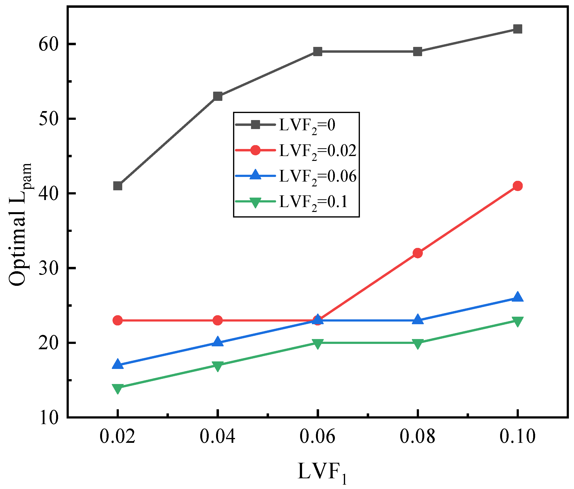
Varied LVF1 with fixed LVF2
Figure 13 is the ER with Lpm under fixed LVF2 of 0.02 and various LVF1. Specifically speaking, for LVF1 of 0.02, the ER reaches the peak value of 1.248 at Lpm = 8 mm. The maximum ER increases by 0.61% compared with the baseline ejector. In terms of LVF1 = 0.04, the ER increases slightly from 0.844 to 0.907, after the highest value, ER drops gradually, and the optimal Lpm is 14 mm in this condition. When LVF1 is in the range of 0.06 to 0.1, as Lpm increases, the increments of the ER do not change a lot. The optimal Lpm are 17 mm, 20 mm, and 23 mm for LVF1 of 0.06, 0.08, and 0.1, respectively. The corresponding maximum ER increases by 1.54%, 3.34%, and 6.65%, respectively. Generally speaking, for LVF2 of 0.02, as LVF1 varies from 0.02 to 0.1, the optimal Lpm, as displayed by the magnified point in Figure 13, becomes larger and larger.
Figure 14 depicts the effect of Lpm on the ER under fixed LVF2 of 0.06 and various LVF1. ERs always increase initially and then decrease. To be specific, for LVF1 of 0.02 and 0.04, both the ERs obtain the maximum value (1.915 and 1.544, respectively) at the Lpm of 5 mm, and the maximum ER increases by 13.58% and 4.17%, respectively. When LVF1 changes from 0.08 to 0.1, ER increases along with the increase of Lpm and obtain the maximum of 1.12 and 0.98, respectively, both the optimum Lpm are 11 mm. Overall, when LVF1 changes from 0.02 to 0.1, the optimal Lpm increases gradually, but all the optimal Lpm are no more than the Lpm of the baseline ejector. Compared with LVF1 = 0.02 as displayed in Figure 13, when LVF2 is 0.06, for each LVF1, all the maximum ERs increase, but optimal Lpm decrease.
Figure 15 displays the impact of Lpm on the ER under LVF2 = 0.1 and various LVF1. The results reveal that all the Ers follow a similar pattern, namely, they increase first and then decrease with the growth of Lpm. For LVF1 varied from 0.02 to 0.06, the maximum Ers (2.2, 1.9, and 1.66, respectively) are all achieved at the Lpm of 5 mm, which is slightly less than the baseline ejector. The maximum ER has an increase of 20.2%, 13.68%, and 6.98%, respectively. Moreover, when LVF1 increases from 0.08 to 0.1, the optimal Lpm increases to 8 mm. The corresponding maximum ERs are 1.47 and 1.32 for LVF1 of 0.08 and 0.1, respectively. In addition, the maximum ER increases by 3.01% and 1.4%, respectively. It is noteworthy that for fixed LVF2 of 0.1 and various LVF1, all the optimal Lpm are less than 11 mm. Compared with Figure 14 in which LVF2 is 0.06, for each LVF1, the maximum ER increases. Moreover, for LVF1 = 0.06–0.1, the optimal Lpm also increases.
Overall, from Figure 13, Figure 14 and Figure 15, it can be inferred that: (1) for each fixed LVF2, the optimal Lpm increases with the growth of LVF1; (2) with the increase of LVF2, the optimal Lpm is generally reduced; (3) when both LVF1 and LVF2 are in the range of 0.02–0.1, the optimal Lpm is in the range of 5–23 mm; (4) and, combined with Figure 6 in which LVF2 is 0, it can also be concluded that the when LVF1 is fixed in the range of 0–0.1, the optimal Lpm improves with the growth of LVF1, and the ER rises with the rise of LVF2.

3.2. Optimization of Lam

Based on the optimal Lpm determined in Section 3.1, the following simulations are performed to seek the optimal Lam.

3.2.1. Effect of Two-Phase Primary Flow

Figure 16 reveals the influence of Lam on ER under various LVF1 (LVF2 = 0). For LVF1 of 0.02 and 0.04, when Lam increases from 9 mm to 24 mm, the influence of Lam is not evident. The ER for LVF1 = 0.02 increases from 0.438 at the Lam of 9 mm to the maximum of 0.442 at the Lam of 18 mm and then drops. For LVF1 = 0.04, the ER rises first and reaches the maximum of 0.24 at Lam = 15 mm and then drops gradually. The optimal Lam for LVF1 of 0.02 and 0.04 are 18 mm and 15 mm, respectively. For LVF1 of 0.06 and 0.08, the optimal Lam are both 15 mm. Nonetheless, when Lam exceeds 15 mm, ER decreases abruptly. For LVF1 of 0.1, the peak value of ER is 0.064 at the Lam of 18 mm, which means the LVF1 = 0.1 has a more evident effect on the ER, the reason is that the liquid density is much higher than the vapor density. Likewise, after the peak value, ER drops suddenly. To avoid the malfunction of the ejector, the Lam should not exceed 15 mm, and the primary flow should not contain liquid. To identify the cause for the abrupt decrease, contours of static pressure, axial static pressure distribution, velocity contours, and the velocity vector field are displayed in Figure 17a–d, respectively. It can be observed from Figure 17a,b that the static pressure monotonically increases in the mixing chamber when Lam is 15 mm and 18 mm. In addition, when Lam rises to 21 mm, the mixed fluids have a momentum drop since the increase of the resistance weakens the ejector performance. In other words, when the friction loss caused by the increase of Lam exceeds the performance enhanced by the effect of more sufficient mixing, the ejector performance will decrease. Moreover, reflux occurs as illustrated in Figure 17d.

3.2.2. Effect of Two-Phase Secondary Flow

Figure 18 displays the effect of Lam on ER under fixed LVF1 of 0 and various LVF2. Obviously, under all the LVF2, ER increases first and then decreases. Nevertheless, for various LVF2, the optimal Lam is not always the same. Specifically, for LVF2 = 0.02, the maximum ER of 2.02 peaks at the Lam of 12 mm. For LVF2 = 0.04, the optimal Lam of 15 mm is the same as that of the baseline ejector. When LVF2 is in the range of 0.06–0.1, the optimal Lam is at 9 mm.

3.2.3. Effect of Two-Phase Primary and Secondary Flows

All the Lam are optimized under LVF1 = 0.02~0.1 and LVF2 = 0.02~0.1 with an interval of 0.02. Considering the limited space, only two cases (LVF1 = 0.1 and LVF2 = 0.02~0.1, LVF2 = 0.1 and LVF1 = 0.02~0.1) are displayed here.
Figure 19 displays the effect of Lam on ER under fixed LVF1 of 0.1 and various LVF2 (0.02–0.1). When Lam increases from 6 mm to 21 mm, for a fixed LVF2, the optimal Lam can be achieved.
Figure 20 presents the effect of Lam on ER under fixed LVF2 of 0.1 and various LVF1 (0.02–0.1). Obviously, for LVF1 = 0.02, 0.04, and 0.06, it can be seen that the change in ER is relatively evident, while for LVF1 = 0.08 and 0.1, the change in ER is pretty small. The results are similar to the variation of the optimal Lam with LVF in Figure 16, Figure 18 and Figure 19, namely the changing trend of optimal Lam is irregular.
In addition, the results of optimal Lam and ER under other LVF are presented in Table 5 and Table 6.
With the results of Section 3.2, it can be found that the relation of optimal Lam with LVF1 and LVF2 is irregular since optimal Lam is influenced by optimal Lpm. When the optimal Lpm is more than 8 mm, the optimization of Lam is not evident, or the influence of Lam is not distinct. Nevertheless, when the optimal Lpm is less than 8 mm, the influence of Lam will be significant. The optimum Lam are in the range of 6–21 mm, and they do not deviate much from the Lam of the baseline ejector model (15 mm).

3.3. A Combination of Optimal Lpm and Lam

Figure 21 depicts the relation of the sum of optimal Lpm and Lam (Lpam) with LVF2 under changed LVF1. It can be observed that for each LVF1, the optimal Lpam decreases with LVF2. Furthermore, the optimal Lpam increases with LVF1.
Figure 22 indicates the relation of the sum of optimal Lpm and Lam with LVF1 under different LVF2. Generally speaking, the optimal Lpam increases with LVF1 but reduces with LVF2, and the relation between optimal Lpm and Lpam is regular.

4. Conclusions

This paper numerically optimizes two mixing chamber geometries of a two-phase ejector under various primary and secondary inlet LVFs. The most important findings are given below:
(1)
When the primary inlet of the ejector contains liquid while the secondary inlet does not, the optimal Lpm and Lam are ranged between 23–44 mm and 15–18 mm. When the secondary inlet contains liquid while primary inlet does not, these two optimal lengths are ranged 2–5 mm and 9–15 mm, while when both the primary inlet and secondary inlet contain liquid, they are in the range of 5–23 mm and 6–18 mm, respectively. Thus, two mixing chamber lengths largely depend on the vapor or liquid state of the two inlets;
(2)
When primary inlet LVF is fixed and secondary inlet LVF increases from 0 to 0.1, the optimal Lpm decreases along with the growth of secondary inlet LVF; when secondary inlet LVF is fixed and primary inlet LVF varies from 0 to 0.1, the optimal Lpm increases along with the growth of primary inlet LVF;
(3)
The sum of optimal Lpm and optimal Lam increases with the increase of primary inlet LVF but decreases with the increase of secondary inlet LVF.

Author Contributions

Conceptualization, J.Y. and J.J.; methodology, H.W.; investigation, J.Y.; writing—original draft preparation, H.W.; writing—review and editing, Y.S. All authors have read and agreed to the published version of the manuscript.

Funding

The research was funded by the Educational Department of Sichuan Province, China (Funding No.: 17ZB0449).

Institutional Review Board Statement

Not applicable.

Informed Consent Statement

Not applicable.

Conflicts of Interest

The authors declare no conflict of interest.

Nomenclature

Lpmconstant-pressure mixing chamber length, mm
Lamconstant-area mixing chamber length, mm
Lpamsum of mixing chamber length, mm
Ppressure, kPa
Ttemperature, K or °C
m1primary mass flow rate, g·s−1
m2secondary mass flow rate, g·s−1
χ quality
α void fraction
ARarea ratio
ERentrainment ratio
PRRpressure recovery ratio
LVF1liquid volume fraction of primary flow
LVF2liquid volume fraction of secondary flow
NXPnozzle exit position
MERSmulti-evaporator refrigeration system

References

  1. Besagni, G.; Mereu, R.; Inzoli, F. Ejector refrigeration: A comprehensive review. Renew. Sustain. Energy Rev. 2016, 53, 373–407. [Google Scholar] [CrossRef] [Green Version]
  2. Wang, J.; Qv, D.; Yao, Y.; Ni, L. The difference between vapor injection cycle with flash tank and intermediate heat exchanger for air source heat pump: An experimental and theoretical study. Energy 2021, 221, 119796. [Google Scholar] [CrossRef]
  3. Cuong, L.N.; Oh, J.T. The Comparison of Experiment Results and CFD Simulation in the Heat Pump System Using Thermobank and Two-Phase Ejector for Heating Room and Cold Storage. Int. J. Air-Cond. Refrig. 2016, 24, 1650004. [Google Scholar] [CrossRef]
  4. Shi, Y.; Guo, X.; Zhang, X. Study on Economized Vapor Injection Heat Pump System Using Refrigerant R32. Int. J. Air-Cond. Refrig. 2016, 24, 1650006. [Google Scholar] [CrossRef]
  5. Gullo, P.; Kærn, M.R.; Haida, M.; Smolka, J.; Elbel, S. A review on current status of capacity control techniques for two-phase ejectors. Int. J. Refrig. 2020, 119, 64–79. [Google Scholar] [CrossRef]
  6. Chen, Q.; Hwang, Y.; Yan, G.; Yu, J. Theoretical investigation on the performance of an ejector enhanced refrigeration cycle using hydrocarbon mixture R290/R600a. Appl. Therm. Eng. 2020, 164, 114456. [Google Scholar] [CrossRef]
  7. Dokandari, D.A.; Khoshkhoo, R.H.; Bidi, M.; Mafi, M. Thermodynamic investigation and optimization of two novel combined power-refrigeration cycles using cryogenic LNG energy. Int. J. Refrig. 2021, 124, 167–183. [Google Scholar] [CrossRef]
  8. Barta, R.B.; Dhillon, P.; Braun, J.E.; Ziviani, D.; Groll, E.A. Design and Optimization Strategy for Ejectors Applied in Refrigeration Cycles. Appl. Therm. Eng. 2021, 189, 116682. [Google Scholar] [CrossRef]
  9. Liu, J.; Lin, Z. A novel dual-temperature ejector-compression heat pump cycle-exergetic and economic analyses. Int. J. Refrig. 2021, 126, 155–167. [Google Scholar] [CrossRef]
  10. Elliott, M.S.; Rasmussen, B.P. Decentralized model predictive control of a multi-evaporator air conditioning system. Control Eng. Pract. 2013, 21, 1665–1677. [Google Scholar] [CrossRef]
  11. Li, C.; Yan, J.; Li, Y.; Cai, W.; Lin, C.; Chen, H. Experimental study on a multi-evaporator refrigeration system with variable area ratio ejector. Appl. Therm. Eng. 2016, 102, 196–203. [Google Scholar] [CrossRef]
  12. Li, S.; Yan, J.; Liu, Z.; Yao, Y.; Li, X.; Wen, N.; Zou, G. Optimization on crucial ejector geometries in a multi-evaporator refrigeration system for tropical region refrigerated trucks. Energy 2019, 189, 116347. [Google Scholar] [CrossRef]
  13. Yan, J.; Li, S.; Li, R. Numerical study on the auxiliary entrainment performance of an ejector with different area ratio. Appl. Therm. Eng. 2020, 185, 116369. [Google Scholar] [CrossRef]
  14. Wen, N.; Wang, L.; Yan, J.; Li, X.; Liu, Z.; Li, S.; Zou, G. Effects of operating conditions and cooling loads on two-stage ejector performances. Appl. Therm. Eng. 2019, 150, 770–780. [Google Scholar] [CrossRef]
  15. Wen, H.; Yan, J.; Li, X. Influence of liquid volume fraction on ejector performance: A numerical study. Appl. Therm. Eng. 2021, 190, 116845. [Google Scholar] [CrossRef]
  16. Kumar, V.; Sachdeva, G. 1-D model for finding geometry of a single phase ejector. Energy 2018, 165, 75–92. [Google Scholar] [CrossRef]
  17. Ramesh, A.S.; Sekhar, S.J. Experimental and numerical investigations on the effect of suction chamber angle and nozzle exit position of a steam-jet ejector. Energy 2018, 164, 1097–1113. [Google Scholar] [CrossRef]
  18. Palacz, M.; Haida, M.; Smolka, J.; Nowak, A.J.; Banasiak, K.; Hafner, A. HEM and HRM accuracy comparison for the simulation of CO2 expansion in two-phase ejectors for supermarket refrigeration systems. Appl. Therm. Eng. 2017, 115, 160–169. [Google Scholar] [CrossRef]
  19. Aidoun, Z.; Ameur, K.; Falsafioon, M.; Badache, M. Current advances in ejector modeling, experimentation and applications for refrigeration and heat pumps. Part 2: Two-phase ejectors. Inventions 2019, 4, 16. [Google Scholar] [CrossRef] [Green Version]
  20. Fu, W.; Li, Y.; Liu, Z.; Wu, H.; Wu, T. Numerical study for the influences of primary nozzle on steam ejector performance. Appl. Therm. Eng. 2016, 106, 1148–1156. [Google Scholar] [CrossRef]
  21. Chunnanond, K.; Aphornratana, S. Ejectors: Applications in refrigeration technology. Renew. Sustain. Energy Rev. 2004, 8, 129–155. [Google Scholar] [CrossRef]
  22. Jeon, Y.; Kim, D.; Jung, J.; Jang, D.S.; Kim, Y. Comparative performance evaluation of conventional and condenser outlet split ejector-based domestic refrigerator-freezers using R600a. Energy 2018, 161, 1085–1095. [Google Scholar] [CrossRef]
  23. Tang, Y.; Liu, Z.; Li, Y.; Huang, Z.; Jon, K. Study on fundamental link between mixing efficiency and entrainment performance of a steam ejector. Energy 2021, 215, 119128. [Google Scholar] [CrossRef]
  24. Nakagawa, M.; Marasigan, A.R.; Matsukawa, T.A. Kurashina, Experimental investigation on the effect of mixing length on the performance of two-phase ejector for CO2 refrigeration cycle with and without heat exchanger. Int. J. Refrig. 2011, 34, 1604–1613. [Google Scholar] [CrossRef]
  25. Sarkar, J. Ejector enhanced vapor compression refrigeration and heat pump systems—A review. Renew. Sustain. Energy Rev. 2012, 16, 6647–6659. [Google Scholar] [CrossRef]
  26. Banasiak, K.; Hafner, A.; Andresen, T. Experimental and numerical investigation of the influence of the two-phase ejector geometry on the performance of the R744 heat pump. Int. J. Refrig. 2012, 35, 1617–1625. [Google Scholar] [CrossRef]
  27. Jeon, Y.; Kim, S.; Kim, D.; Chung, H.J.; Kim, Y. Performance characteristics of an R600a household refrigeration cycle with a modified two-phase ejector for various ejector geometries and operating conditions. Appl. Energy 2017, 205, 1059–1067. [Google Scholar] [CrossRef]
  28. Fu, W.; Liu, Z.; Li, Y.; Wu, H.; Tang, Y. Numerical study for the influences of primary steam nozzle distance and mixing chamber throat diameter on steam ejector performance. Int. J. Therm. Sci. 2018, 132, 509–516. [Google Scholar] [CrossRef]
  29. Dong, J.; Hu, Q.; Yu, M.; Han, Z.; Cui, W.; Liang, D.; Ma, H.; Pan, X. Numerical investigation on the influence of mixing chamber length on steam ejector performance. Appl. Therm. Eng. 2020, 174, 115204. [Google Scholar] [CrossRef]
  30. Hemidi, A.; Henry, F.; Leclaire, S.; Seynhaeve, J.M.; Bartosiewicz, Y. CFD analysis of a supersonic air ejector. Part I: Experimental validation of single-phase and two-phase operation. Appl. Therm. Eng. 2009, 29, 1523–1531. [Google Scholar] [CrossRef]
  31. Yuan, G.; Zhang, L.; Zhang, H.; Wang, Z. Numerical and experimental investigation of performance of the liquid-gas and liquid jet pumps in desalination systems. Desalination 2011, 276, 89–95. [Google Scholar] [CrossRef]
  32. Chen, W.; Huang, C.; Bai, Y.; Chong, D.; Yan, J.; Liu, J. Experimental and numerical investigation of two phase ejector performance with the water injected into the induced flow. Int. J. Adv. Nucl. React. Des. Technol. 2020, 2, 15–24. [Google Scholar] [CrossRef]
  33. Aliabadi, M.A.F.; Bahiraei, M. Effect of water nano-droplet injection on steam ejector performance based on non-equilibrium spontaneous condensation: A droplet number study. Appl. Therm. Eng. 2021, 184, 116236. [Google Scholar] [CrossRef]
  34. Yan, J.; Li, S.; Liu, Z. Numerical investigation on optimization of ejector primary nozzle geometries with fixed/varied nozzle exit position. Appl. Therm. Eng. 2020, 175, 115426. [Google Scholar] [CrossRef]
  35. Li, C.; Li, Y.Z. Investigation of entrainment behavior and characteristics of gas-liquid ejectors based on CFD simulation. Chem. Eng. Sci. 2011, 66, 405–416. [Google Scholar] [CrossRef]
  36. Palacz, M.; Smolka, J.; Kus, W.; Fic, A.; Bulinski, Z.; Nowak, A.J.; Banasiak, K.; Hafner, A. CFD-based shape optimisation of a CO2 two-phase ejector mixing section. Appl. Therm. Eng. 2016, 95, 62–69. [Google Scholar] [CrossRef]
  37. Besagni, G.; Cristiani, N.; Croci, L.; Guédon, G.R.; Inzoli, F. Computational fluid-dynamics modelling of supersonic ejectors: Screening of modelling approaches, comprehensive validation and assessment of ejector component efficiencies. Appl. Therm. Eng. 2021, 186, 116431. [Google Scholar] [CrossRef]
  38. Carrillo, J.A.E.; de la Flor, F.J.S.; Lissén, J.M.S. Single-phase ejector geometry optimisation by means of a multi-objective evolutionary algorithm and a surrogate CFD model. Energy 2018, 164, 46–64. [Google Scholar] [CrossRef]
  39. Croquer, S.; Poncet, S.; Aidoun, Z. Turbulence modeling of a single-phase R134a supersonic ejector. Part 1: Numerical benchmark. Int. J. Refrig. 2016, 61, 140–152. [Google Scholar] [CrossRef]
Figure 1. Schematic of a two-temperature evaporator-based EMERS.
Entropy 25 00007 g001
Figure 2. Schematic of the ejector.
Entropy 25 00007 g002
Figure 3. Densified meshes of the ejector.
Entropy 25 00007 g003
Figure 4. Comparison of α between simulation and correlation results.
Entropy 25 00007 g004
Figure 5. The relation of mass flow rate and ER with diverging section length of the primary nozzle.
Entropy 25 00007 g005
Figure 6. The Mach number contours under different nozzle diverging section lengths: (a) 0 mm; (b) 2 mm; (c) 4 mm; and (d) 6 mm.
Entropy 25 00007 g006
Figure 7. Optimization of Lpm on ER under LVF1 = 0.02~0.1 (LVF2 = 0).
Entropy 25 00007 g007
Figure 8. Pressure inside the ejector with different Lpm under LVF1 = 0.06 and LVF2 = 0: (a) Contour of static pressure; (b) Static pressure along the centerline; (c) Contour of velocity.
Entropy 25 00007 g008aEntropy 25 00007 g008b
Figure 9. Optimization of Lpm on ER with LVF1 = 0 and LVF2 = 0.02~0.1.
Entropy 25 00007 g009
Figure 10. The relation of ER with Lpm under LVF1 = 0.02 and LVF2 = 0.02~0.1.
Entropy 25 00007 g010
Figure 11. The relation of ER with Lpm under LVF1 = 0.06 and LVF2 = 0.02~0.1.
Entropy 25 00007 g011
Figure 12. The relation of ER with Lpm under LVF1 = 0.1 and various LVF2.
Entropy 25 00007 g012
Figure 13. The relation of ER with Lpm under LVF2 = 0.02 and LVF1 = 0.02~0.1.
Entropy 25 00007 g013
Figure 14. The relation of ER with Lpm under LVF2 = 0.06 and LVF1 = 0.02~0.1.
Entropy 25 00007 g014
Figure 15. The variation of ER with Lpm under LVF2 = 0.1 and LVF1 = 0.02~0.1.
Entropy 25 00007 g015
Figure 16. ER with Lam under LVF1 = 0.02~0.1 (LVF2 = 0).
Entropy 25 00007 g016
Figure 17. Pressure inside the ejector with different Lam under LVF1 = 0.1 and LVF2 = 0: (a) Contour of static pressure; (b) Static pressure along the centerline; (c) Contour of velocity and (d) Velocity vector field of Lam = 21 mm.
Entropy 25 00007 g017aEntropy 25 00007 g017b
Figure 18. ER with Lam under LVF2 = 0.02~0.1 (LVF1 = 0).
Entropy 25 00007 g018
Figure 19. The relation of ER with Lam under LVF1 = 0.1 and LVF2 = 0.02~0.1.
Entropy 25 00007 g019
Figure 20. The relation of ER with Lam under LVF2 = 0.1 and LVF1 = 0.02~0.1.
Entropy 25 00007 g020
Figure 21. The relation of optimal Lpam with LVF2 under different LVF1.
Entropy 25 00007 g021
Figure 22. The relation of optimal Lpam with LVF1 under given LVF2.
Entropy 25 00007 g022
Table 1. Initial geometrical parameters of the ejector.
ParametersValue (mm)
The suction chamber diameter, Ds19.6
The primary nozzle inlet diameter, Dp9.6
The primary nozzle outlet diameter, Dn3
The constant-area mixing chamber diameter, Dam5.2
The diffuser outlet diameter, Dd10
The primary nozzle length, Lp20
The constant-pressure mixing chamber length, Lpm11
The constant-area mixing chamber length, Lam15
The diffuser length, Ld56
Table 2. Boundary conditions for the ejector.
ParametersTypePressure (kPa)Temperature (K)
Superheated GasTwo-Phase
Primary inletPressure inlet374.6290280
Secondary inletPressure inlet243.3278268
OutletPressure outlet267.63--
Table 3. Mesh sensitivity analysis of area A.
Grid NumberPressure (Pa)Error (%)Velocity (m·s−1)Error (%)
52,200274,947-120.138-
68,520275,2880.12119.8930.2
83,100275,5210.085119.6840.17
114,880275,6130.033119.6230.051
Table 4. Mesh sensitivity analysis of area B.
Grid NumberPressure (Pa)Error (%)Velocity (m·s−1)Error (%)
52,200206,538-165.218-
68,520206,8790.165164.9340.172
83,100207,0540.085164.8410.056
114,880207,1230.033164.7880.032
Table 5. Results of optimal Lam and maximum ER under varied LVF1 for a given LVF2.
LVF2 = 0
(ER)
LVF2 = 0.02
(ER)
LVF2 = 0.06 (ER)LVF2 = 0.1 (ER)
LVF1 = 0.0218 (0.442)15 (1.248)12 (1.941)9 (2.344)
LVF1 = 0.0421 (0.24)9 (0.912)15 (1.544)12 (1.932)
LVF1 = 0.0615 (0.145)6 (0.693)15 (1.306)15 (1.661)
LVF1 = 0.0815 (0.092)12 (0.536)12 (1.128)12 (1.474)
LVF1 = 0.118 (0.065)18 (0.423)15 (0.983)15 (1.321)
Table 6. Results of optimal Lam and maximum ER under varied LVF2 for a given LVF1.
LVF1 = 0
(ER)
LVF1 = 0.02
(ER)
LVF1 = 0.06 (ER)LVF1 = 0.1 (ER)
LVF2 = 0.0212 (2.02)15 (1.248)6 (0.693)18 (0.423)
LVF2 = 0.0415 (2.362)15 (1.651)12 (1.055)12 (0.744)
LVF2 = 0.069 (2.687)12 (1.941)15 (1.306)15 (0.983)
LVF2 = 0.089 (2.958)9 (2.158)12 (1.504)12 (1.172)
LVF2 = 0.19 (3.17)9 (2.344)15 (1.661)15 (1.321)
Disclaimer/Publisher’s Note: The statements, opinions and data contained in all publications are solely those of the individual author(s) and contributor(s) and not of MDPI and/or the editor(s). MDPI and/or the editor(s) disclaim responsibility for any injury to people or property resulting from any ideas, methods, instructions or products referred to in the content.

