
Physics-Informed Neural Networks for Solving Coupled Stokes–Darcy Equation

Abstract
:1. Introduction
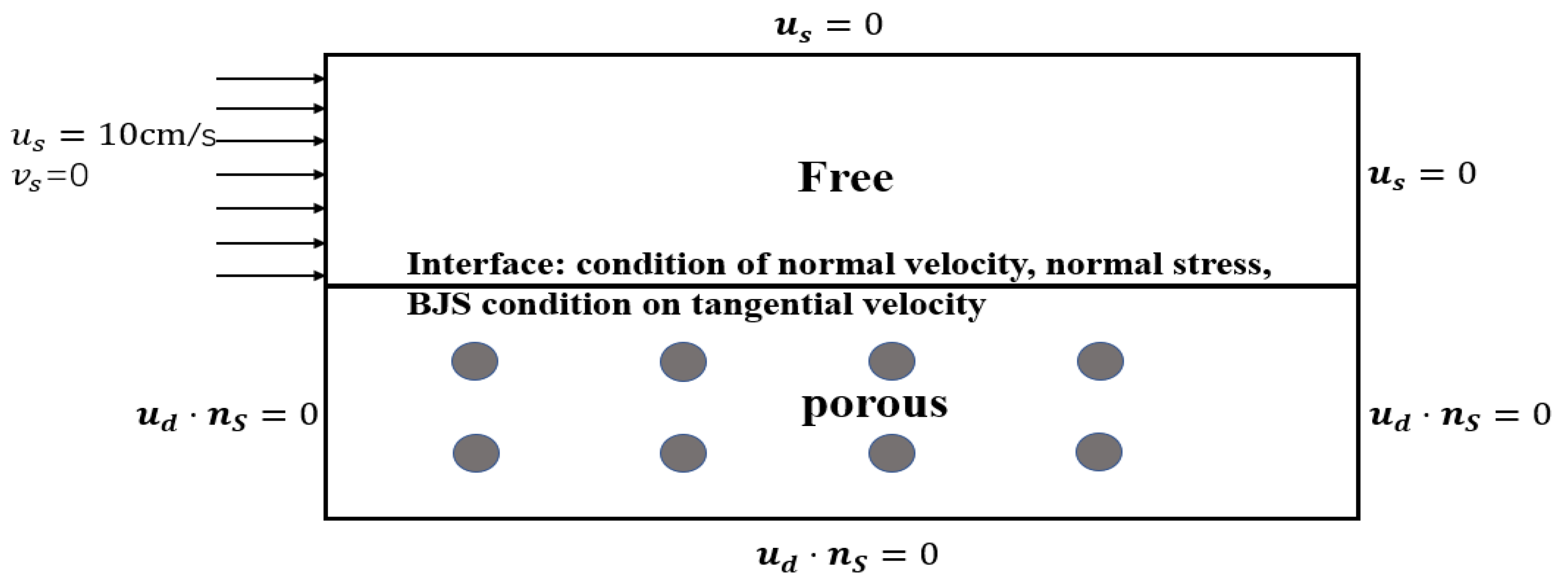
2. Problem Setup
3. Numerical Method
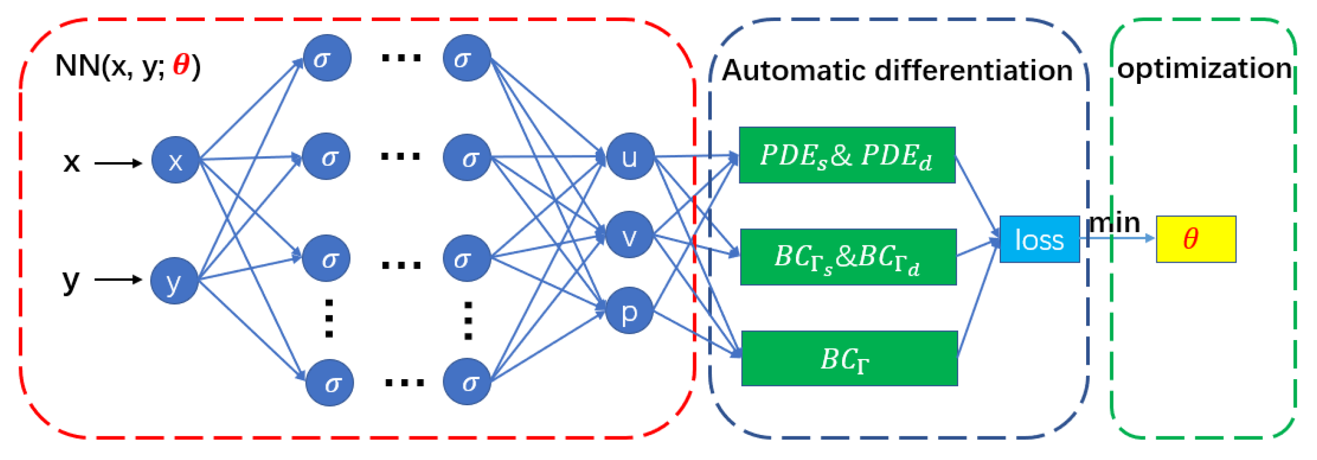
3.1. Network Formation
3.2. Physics-Informed Neural Networks
3.3. Improving Strategy of Physical-Informed Neural Network
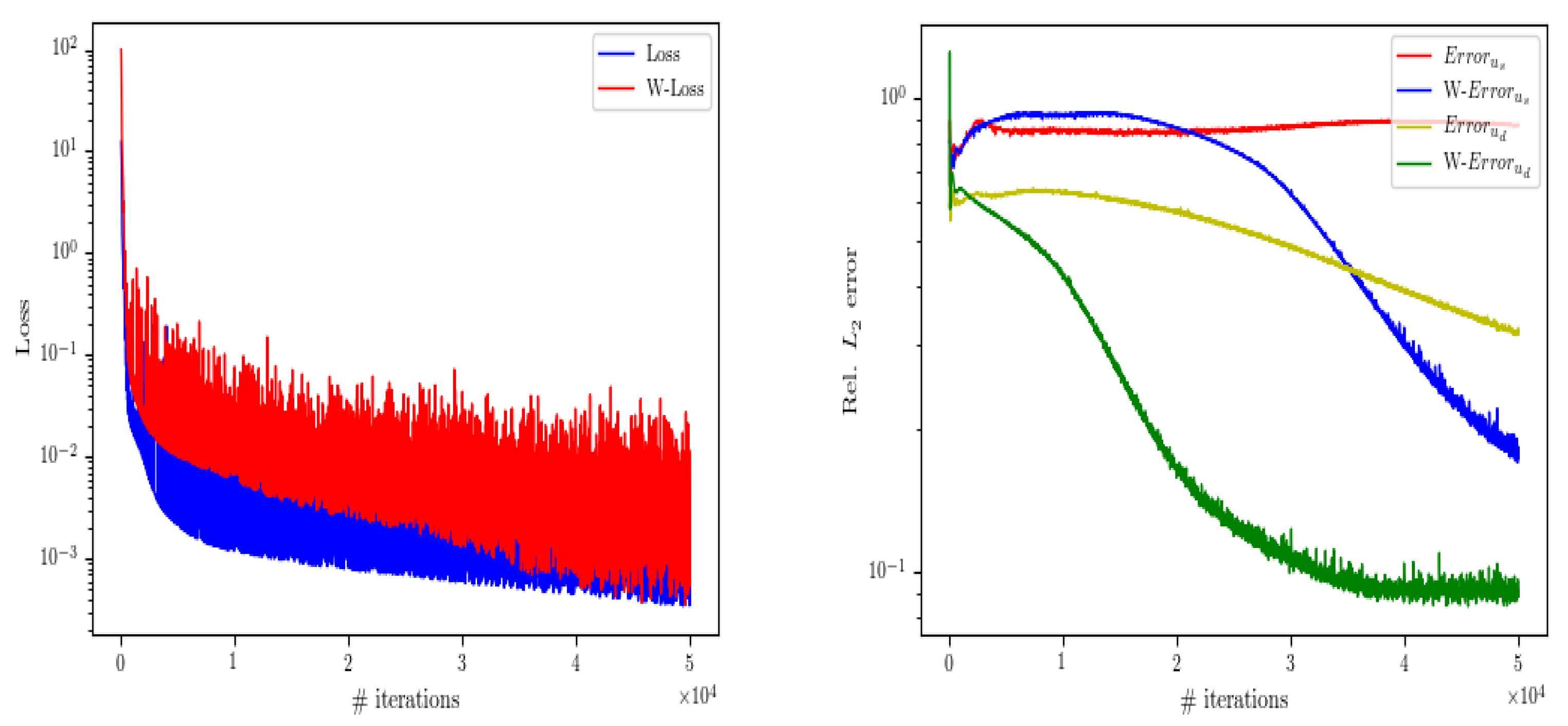
3.3.1. Add a Weight Function to the Loss Function
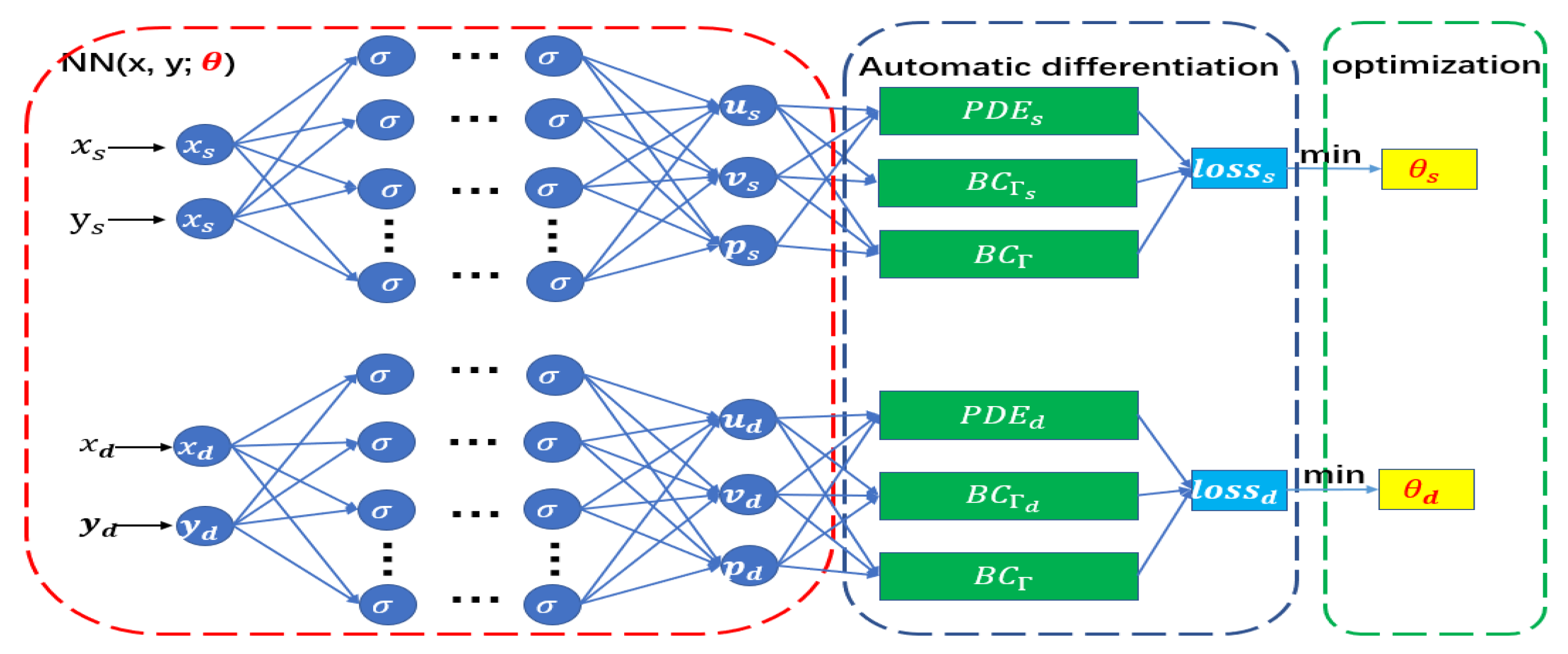
3.3.2. Parallel Network Architecture
3.3.3. Local Adaptive Activation Function Strategy
4. Numerical Experiments
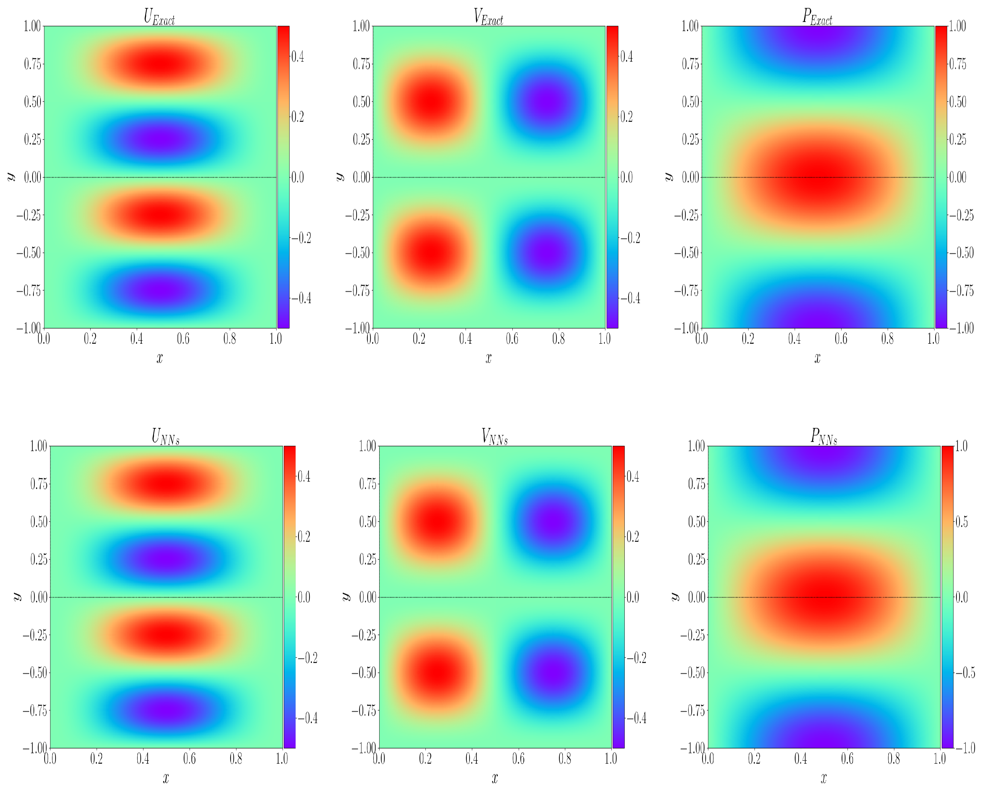
4.1. Interface Continuous Solution Problem
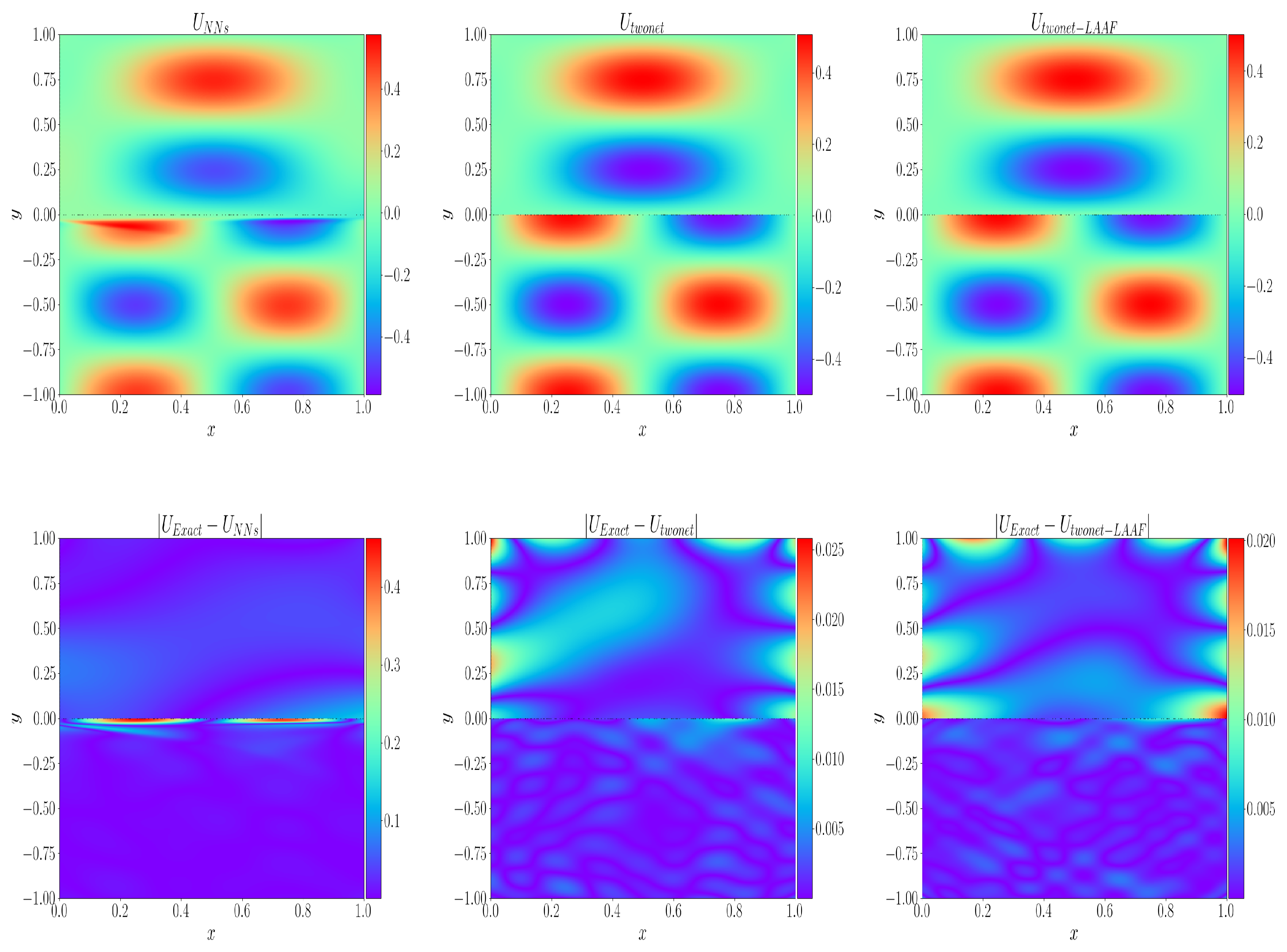
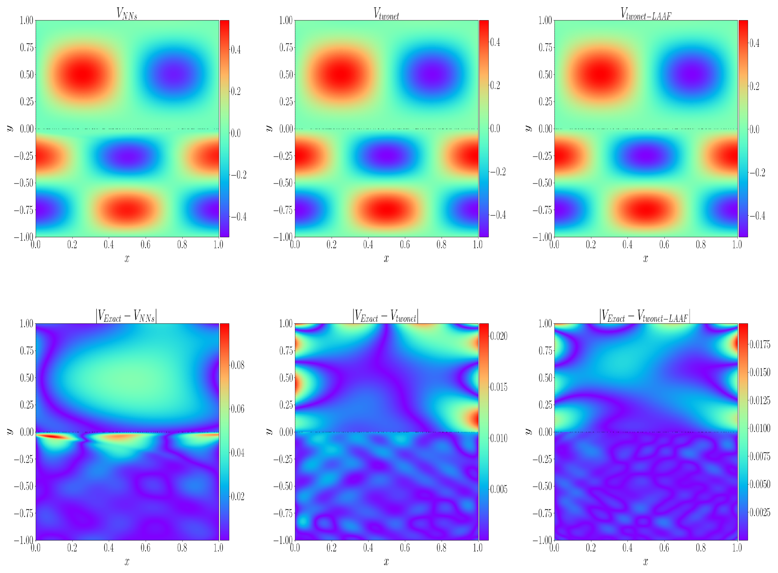
4.2. Interface Discontinuity Solution Problem
4.3. Curved Interface Problem
4.4. No-True Solution Problem
5. Conclusions
Author Contributions
Funding
Acknowledgments
Conflicts of Interest
References
- Yarotsky, D. Error bounds for approximations with deep ReLU networks. Neural Netw. 2017, 94, 103–114. [Google Scholar] [CrossRef] [PubMed]
- Chen, W.B.; Wang, F.; Wang, Y.Q. Weak Galerkin method for the coupled Darcy-Stokes flow. IMA J. Numer. Anal. 2016, 36, 897–921. [Google Scholar] [CrossRef]
- Chen, W.B.; Gunzburger, M.; Hua, F.; Wang, X. A parallel robin-robin domain decomposition method for the Stokes–Darcy system. IMA J. Numer. Anal. 2011, 49, 1064–1084. [Google Scholar] [CrossRef]
- Discacciati, M.; Quarteroni, A. Convergence analysis of a subdomain iterative method for the finite element approximation of the coupling of Stokes and Darcy equations. Comput. Vis. Sci. 2004, 6, 93–103. [Google Scholar] [CrossRef]
- Discacciati, M.; Miglio, E.; Quarteroni, A. Mathematical and numerical models for coupling surface and groundwater flows. Appl. Numer. Math. 2002, 43, 57–74. [Google Scholar] [CrossRef]
- Jiang, B. A parallel domain decomposition method for coupling of surface and groundwater flows. Comput. Method Appl. Mech. Eng. 2009, 198, 947–957. [Google Scholar] [CrossRef]
- Kanschat, G.; Rivière, B. A strongly conservative finite element method for the coupling of Stokes and Darcy flow. J. Comput. Phys. 2010, 229, 5933–5943. [Google Scholar] [CrossRef]
- Goodfellow, I.; Bengio, Y.; Courville, A. Deep Learning; MIT Press: Cambrigde, MA, USA, 2016. [Google Scholar]
- Lecun, Y.; Bengio, Y.; Hinton, G. Deep learning. Nature 2015, 521, 436–444. [Google Scholar] [CrossRef]
- Dockhorn, T. A discussion on solving partial differential equations using neural networks. arXiv 2022, arXiv:1904.07200. [Google Scholar]
- Berg, J.; Nyström, K. Data-driven discovery of PDEs in complex datasets. J. Comput. Phys. 2019, 384, 239–252. [Google Scholar] [CrossRef]
- Sirignano, J.; Spiliopoulos, K. A deep learning algorithm for solving partial differential equations. J. Comput. Phys. 2018, 375, 1339–1364. [Google Scholar] [CrossRef]
- Yu, B. The deep Ritz method: A deep learning-based numerical algorithm for solving variational problems. Commun. Math. Stat. 2018, 6, 1–12. [Google Scholar]
- Raissi, M.; Perdikaris, P.; Karniadakis, G.E. Physics-informed neural networks: A deep learning framework for solving forward and inverse problems involving nonlinear partial differential equations. J. Comput. Phys. 2019, 378, 686–707. [Google Scholar] [CrossRef]
- Dwivedi, V.; Parashar, N.; Srinivasan, B. Distributed physics informed neural network for data-efficient solution to partial differential equations. arXiv 2019, arXiv:1907.08967. [Google Scholar]
- Jagtap, A.D.; Karniadakis, G.E. Extended physics-informed neural networks (XPINNs): A generalized space-time domain decomposition based deep learning framework for nonlinear partial differential equations. Commun. Comput. Phys. 2020, 28, 2002–2041. [Google Scholar]
- Jin, X.; Cai, S.; Li, H.; Karniadakis, G.E. NSFnets (Navier–Stokes Flow nets): Physics-informed neural networks for the incompressible Navier–Stokes equations. J. Comput. Phys. 2021, 426, 109951. [Google Scholar] [CrossRef]
- Kharazmi, E.; Zhang, Z.; Karniadakis, G.E. Variational physics-informed neural networks for solving partial differential equations. arXiv 2019, arXiv:1912.00873. [Google Scholar]
- Meng, X.; Li, Z.; Zhang, D.; Karniadakis, G.E. PPINN: Parareal physics-informed neural network for time-dependent PDEs. Comput. Method Appl. Mech. Eng. 2020, 370, 113250. [Google Scholar] [CrossRef]
- Shukla, K.; Jagtap, A.D.; Blackshire, J.L.; Sparkman, D.; Karniadakis, G.E. A Physics-Informed Neural Network for Quantifying the Microstructural Properties of Polycrystalline Nickel Using Ultrasound Data: A promising approach for solving inverse problems. IEEE. Signal. Proc. Mag. 2021, 39, 68–77. [Google Scholar] [CrossRef]
- Jagtap, A.D.; Mitsotakis, D.; Karniadakis, G.E. Deep learning of inverse water waves problems using multi-fidelity data: Application to Serre–Green–Naghdi equations. Ocean. Eng. 2022, 248, 110775. [Google Scholar] [CrossRef]
- Jagtap, A.D.; Mao, Z.; Adams, N.; Karniadakis, G.E. Physics-informed neural networks for inverse problems in supersonic flows. J. Comput. Phys. 2022, 466, 111402. [Google Scholar] [CrossRef]
- Wang, S.; Yu, X.; Perdikaris, P. When and why pinns fail to train: A neural tangent kernel perspective. J. Comput. Phys. 2022, 499, 110768. [Google Scholar] [CrossRef]
- Mao, Z.; Jagtap, A.D.; Karniadakis, G.E. Physics-informed neural networks for high-speed flows. Comput. Method Appl. Mech. Eng. 2020, 360, 112789. [Google Scholar] [CrossRef]
- Lu, L.; Meng, X.; Mao, Z.; Karniadakis, G.E. DeepXDE: A deep learning library for solving differential equations. SIAM Rev. 2021, 63, 208–228. [Google Scholar] [CrossRef]
- Mishra, S.; Molinaro, R. Estimates on the generalization error of physics-informed neural networks for approximating a class of inverse problems for PDEs. IMA J. Numer. Anal. 2022, 42, 981–1022. [Google Scholar] [CrossRef]
- De Ryck, T.; Jagtap, A.D.; Mishra, S. Error estimates for physics informed neural networks approximating the Navier–Stokes equations. arXiv 2022, arXiv:2203.09346. [Google Scholar]
- Hu, Z.; Jagtap, A.D.; Karniadakis, G.E.; Kawaguchi, K. When do extended physics-informed neural networks (XPINNs) improve generalization? arXiv 2021, arXiv:2109.09444. [Google Scholar]
- Wang, Z.; Zhang, Z. A mesh-free method for interface problems using the deep learning approach. J. Comput. Phys. 2020, 400, 108963. [Google Scholar] [CrossRef]
- Rui, H.; Zhang, R. A unified stabilized mixed finite element method for coupling Stokes and Darcy flows. Comput. Method Appl. Mech. Eng. 2009, 198, 2692–2699. [Google Scholar] [CrossRef]
- Arbogast, T.; Brunson, D.S. A computational method for approximating a Darcy-Stokes system governing a vuggy porous medium. Computat. Geosci. 2007, 11, 207–218. [Google Scholar] [CrossRef]
- Vassilev, D.; Yotov, I. Coupling Stokes–Darcy flow with transport. SIAM J. Sci. Comput. 2009, 31, 3661–3684. [Google Scholar] [CrossRef]
- Jäger, W.; Mikelic, A. On the interface boundary condition of Beavers, Joseph, and Saffman. SIAM J. Appl. Math. 2000, 60, 1111–1127. [Google Scholar]
- Beavers, G.S.; Joseph, D.D. Boundary conditions at a naturally permeable wall. J. Fluid Mech. 1967, 30, 197–207. [Google Scholar] [CrossRef]
- Saffman, P.G. On the boundary condition at the surface of a porous medium. Stud. Appl. Math. 1971, 50, 93–101. [Google Scholar] [CrossRef]
- Baydin, A.G.; Pearlmutter, B.A.; Radul, A.A.; Siskind, J.M. Automatic differentiation in machine learning: A survey. J. Mach. Learn. Res. 2017, 18, 5595–5637. [Google Scholar]
- Kingma, D.P.; Ba, J.L. Adam: A method for stochastic optimization. arXiv 2014, arXiv:1412.6980. [Google Scholar]
- Zhu, C.; Byrd, R.H.; Lu, P.; Nocedal, J. Algorithm 778: L-BFGS-B: Fortran subroutines for large-scale bound-constrained optimization. ACM. Trans. Math. Softw. 1997, 23, 550–560. [Google Scholar] [CrossRef]
- Wang, S.; Teng, Y.; Perdikaris, P. Understanding and mitigating gradient flow pathologies in physics-informed neural networks. SIAM J. Sci. Comput. 2021, 43, A3055–A3081. [Google Scholar] [CrossRef]
- McClenny, L.; Braga-Neto, U. Self-Adaptive Physics-Informed Neural Networks using a Soft Attention Mechanism. arXiv 2020, arXiv:2009.04544. [Google Scholar]
- Jagtap, A.D.; Kharazmi, E.; Karniadakis, G.E. Conservative physics-informed neural networks on discrete domains for conservation laws: Applications to forward and inverse problems. Comput. Method Appl. Mech. Eng. 2020, 365, 113028. [Google Scholar] [CrossRef]
- Shukla, K.; Jagtap, A.D.; Karniadakis, G.E. Parallel physics-informed neural networks via domain decomposition. J. Comput. Phys. 2021, 447, 110683. [Google Scholar] [CrossRef]
- Jagtap, A.D.; Shin, Y.; Kawaguchi, K. Deep Kronecker neural networks: A general framework for neural networks with adaptive activation functions. Neurocomputing 2022, 468, 165–180. [Google Scholar] [CrossRef]
- Jagtap, A.D.; Kawaguchi, K.; Karniadakis, G.E. Adaptive activation functions accelerate convergence in deep and physics-informed neural networks. J. Sci. Comput. 2020, 404, 109136. [Google Scholar] [CrossRef]


| 500 | 125 | 15,000 | 5 | 100 | Adam&L-BFGS | 30,903 |
| , | ||||||||
|---|---|---|---|---|---|---|---|---|
| , | ||||||||
|---|---|---|---|---|---|---|---|---|
| [2] + 4 × [10] + [3] | ||||
| [2] + 4 × [20] + [3] | ||||
| [2] + 4 × [40] + [3] | ||||
| [2] + 4 × [60] + [3] | ||||
| [2] + 4 × [80] + [3] |
| [2] + 2 × [60] + [3] | ||||
| [2] + 4 × [60] + [3] | ||||
| [2] + 6 × [60] + [3] | ||||
| [2] + 8 × [60] + [3] |
| Single Network | Parallel Network, a = 1 | Variable a, (n = 20) | |
|---|---|---|---|
| network architecture | [2] + 4 × [100] + [3] | [2] + 4 × [70] + [3] (double) | [2] + 4 × [70] + [3] (double) |
| 30,903 | 30,666 | 30,666 | |
| Training times | 50,000 | 50,000 | 50,000 |
| N | 31,000 | 31,000 | 31,000 |
| CPU-time(s) | 11,482.7207 | 8482.6347 | 10,607.3143 |
| 500 | 200 | 15,000 | 5 | 100 | 30,903 |
| 375 | 125 | 15,000 | 5 | 100 | 30,903 |
Publisher’s Note: MDPI stays neutral with regard to jurisdictional claims in published maps and institutional affiliations. |
© 2022 by the authors. Licensee MDPI, Basel, Switzerland. This article is an open access article distributed under the terms and conditions of the Creative Commons Attribution (CC BY) license (https://creativecommons.org/licenses/by/4.0/).
Share and Cite
Pu, R.; Feng, X. Physics-Informed Neural Networks for Solving Coupled Stokes–Darcy Equation. Entropy 2022, 24, 1106. https://doi.org/10.3390/e24081106
Pu R, Feng X. Physics-Informed Neural Networks for Solving Coupled Stokes–Darcy Equation. Entropy. 2022; 24(8):1106. https://doi.org/10.3390/e24081106
Chicago/Turabian StylePu, Ruilong, and Xinlong Feng. 2022. "Physics-Informed Neural Networks for Solving Coupled Stokes–Darcy Equation" Entropy 24, no. 8: 1106. https://doi.org/10.3390/e24081106