
Differential Expression Analysis of Single-Cell RNA-Seq Data: Current Statistical Approaches and Outstanding Challenges


Abstract
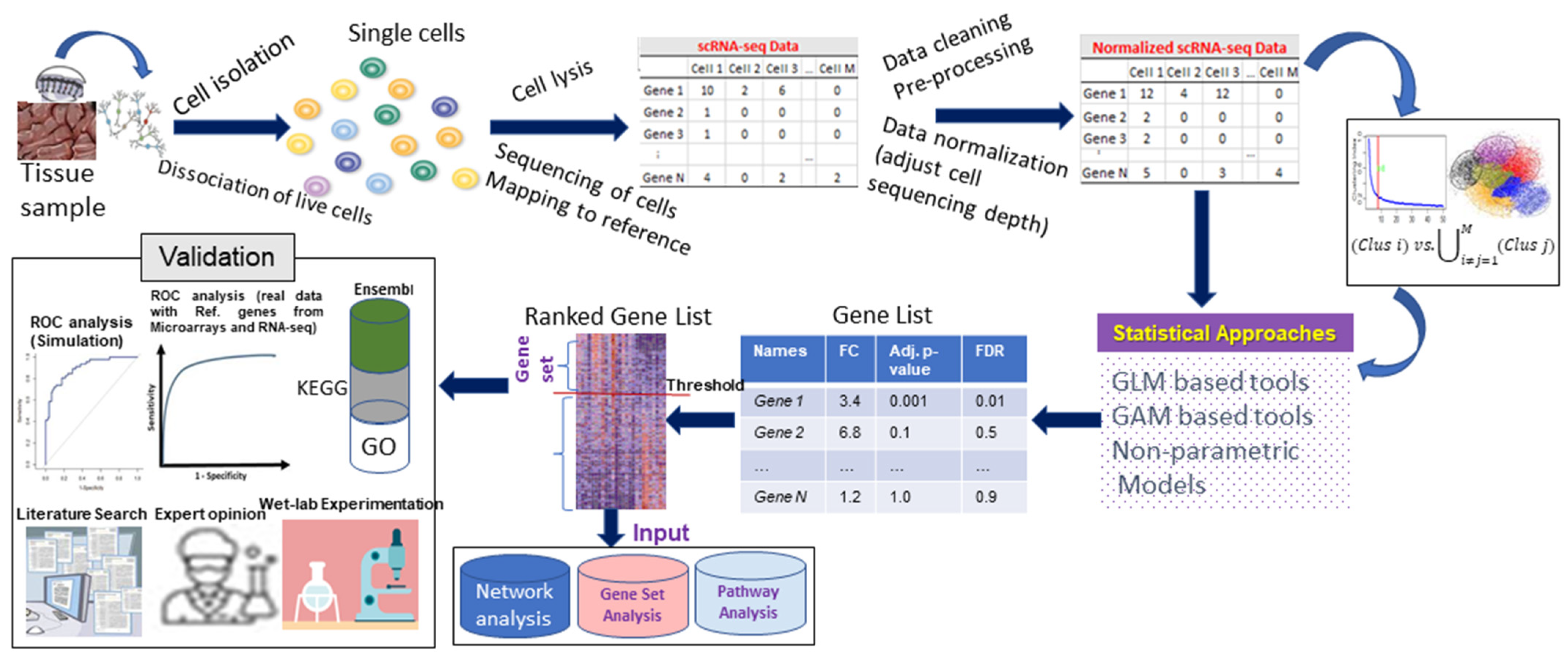
:1. Background
2. Current Statistical Approaches
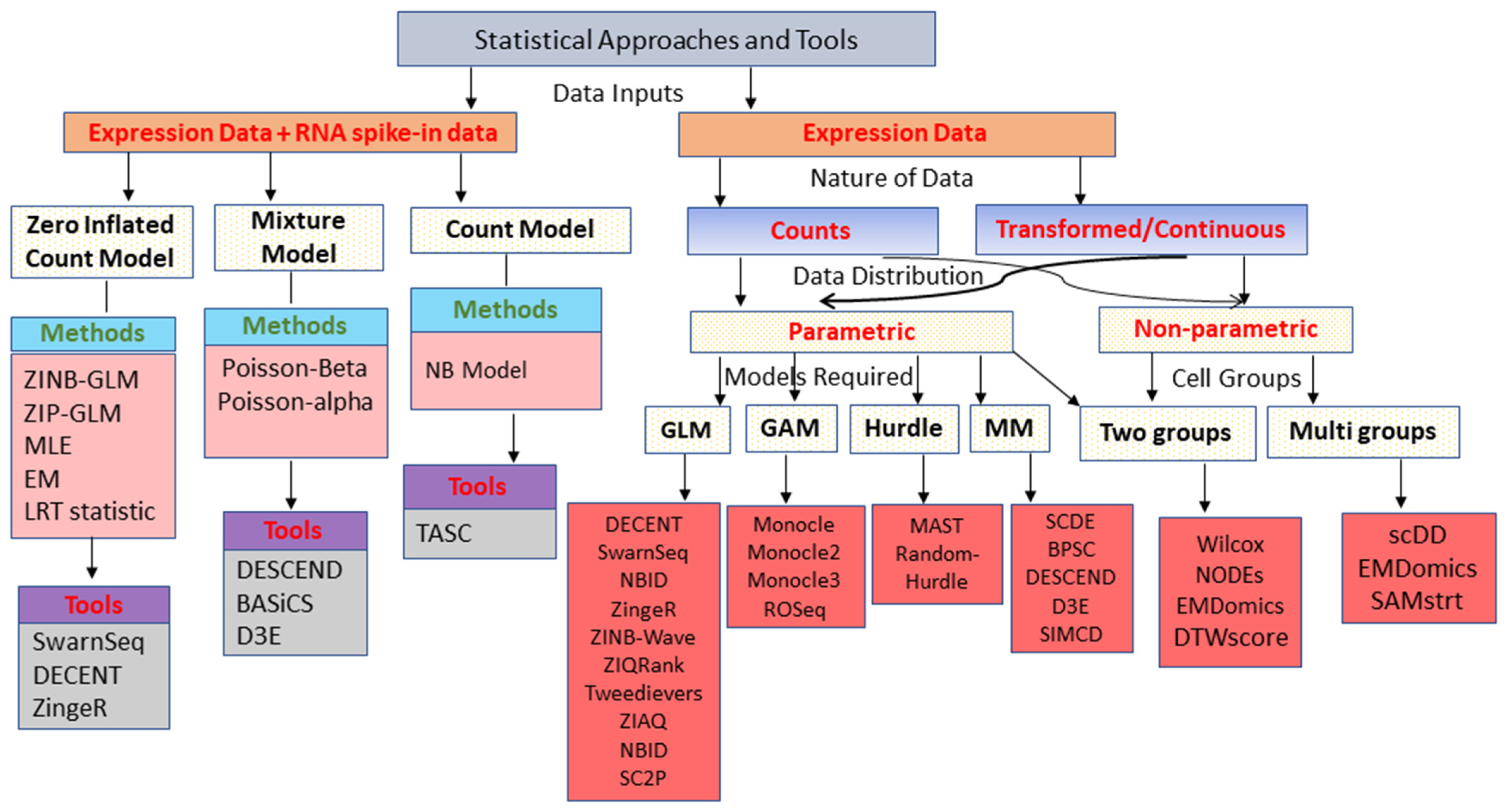
3. Classes of Statistical Approaches for DEA
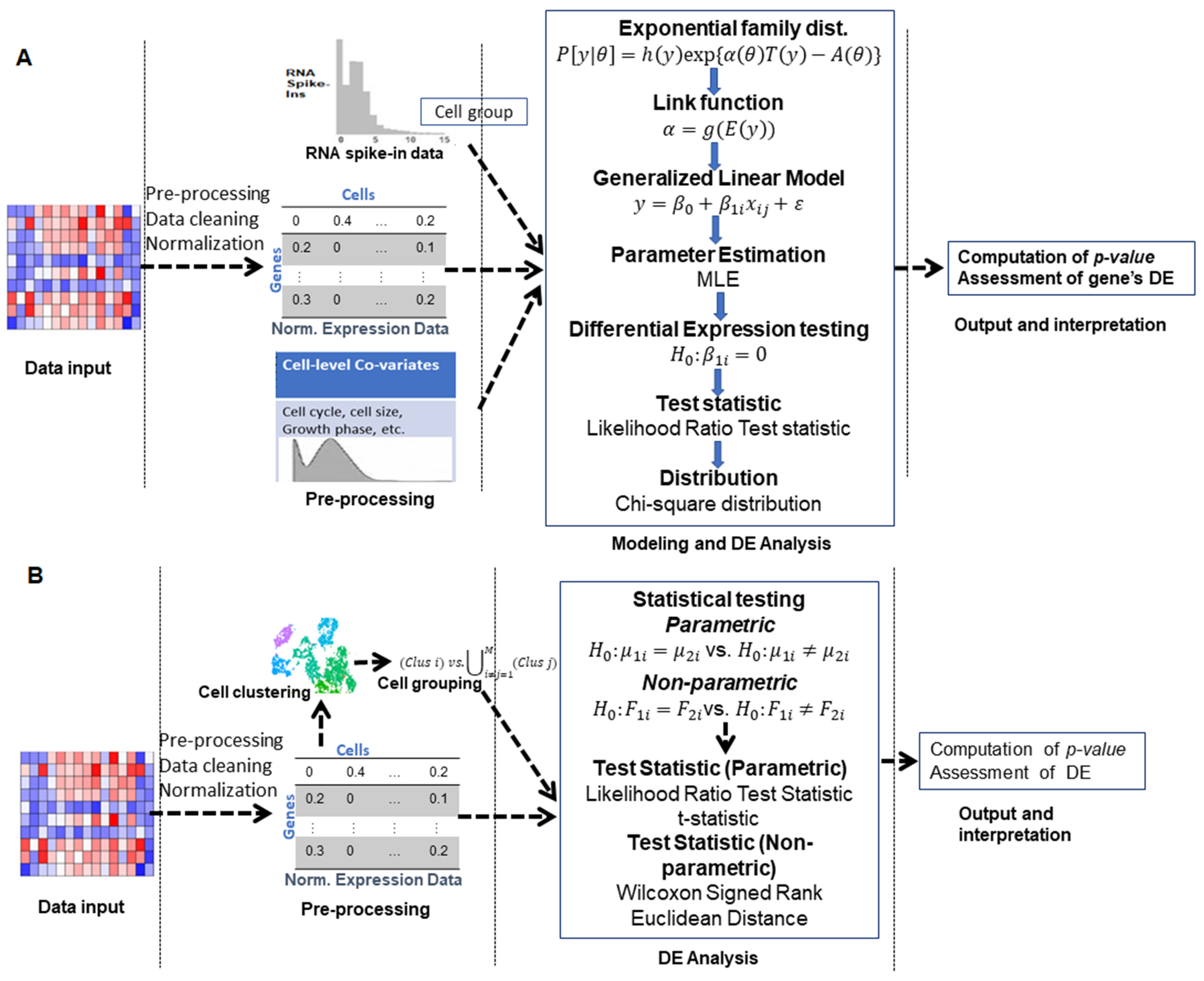
3.1. Generalized Linear Model-Based Approaches
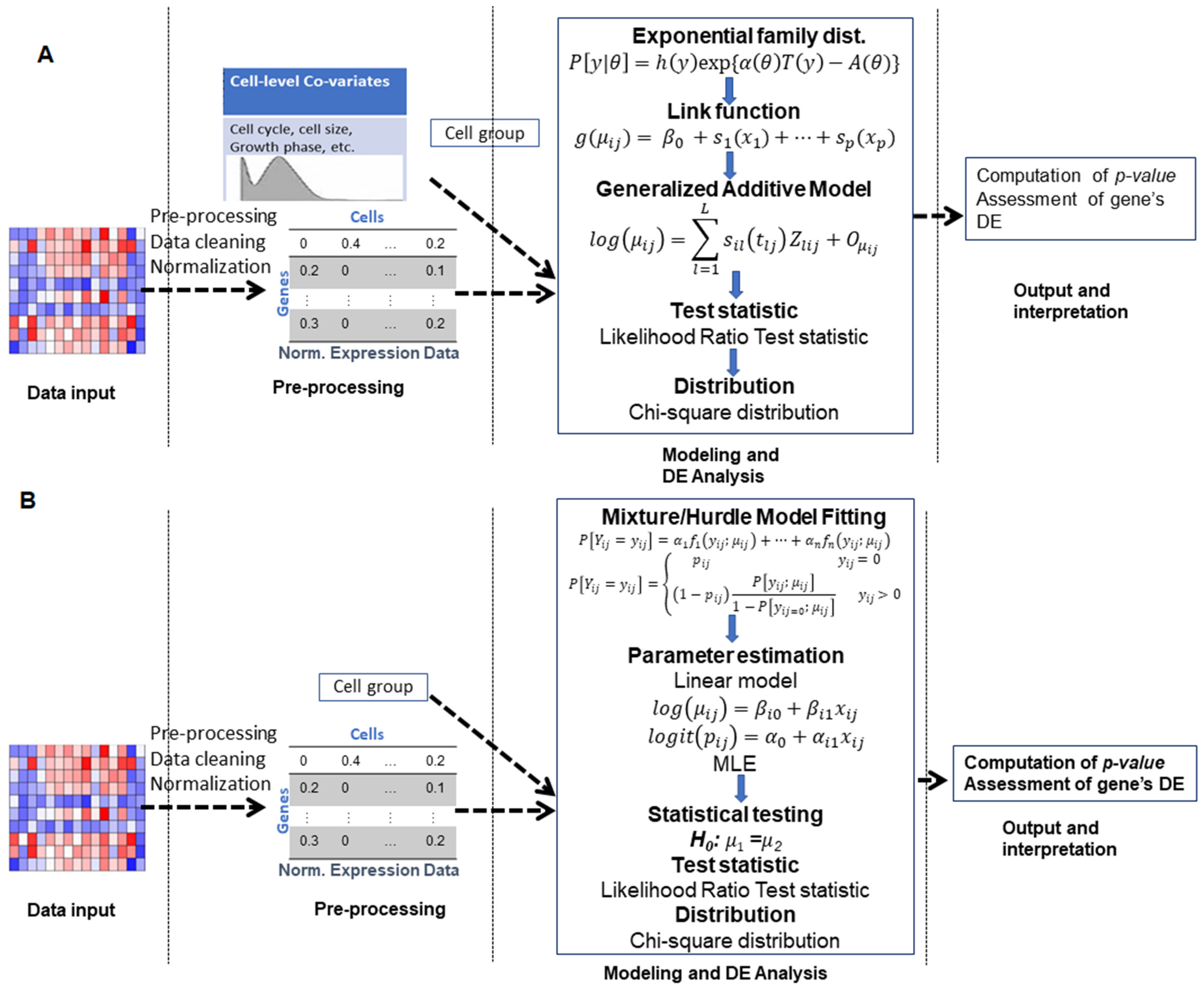
3.2. Generalized Additive Model-Based Approaches
3.3. Mixture Model-Based Approaches
3.4. Hurdle Model-Based Approaches
3.5. Two-Class Comparison (Parametric) Approaches
3.6. Non-Parametric Approaches
4. Outstanding Challenges
4.1. Biological Challenges
4.1.1. Proper Biological Benchmarking
4.1.2. Annotation
4.2. Methodological Challenges
4.2.1. Gold Standard scRNA-seq Data
4.2.2. Excess Heterogeneity
4.2.3. Dropouts or Excess Zeros of Single-Cell Data
4.2.4. Pre-Processing of scRNA-seq Data
4.2.5. Lack of Biological Relevant Criteria
4.2.6. Statistical Methods for DEA across Individuals
4.2.7. False Discoveries in DEA
4.2.8. Improved Methods for Dispersion Estimation
4.2.9. Random/Mixed Effect Models
4.2.10. Optimal Combination of Algorithms
4.2.11. Integration of Multi-Omics Data
4.2.12. Slow Computational Processing
5. Conclusions
Supplementary Materials
Author Contributions
Funding
Institutional Review Board Statement
Informed Consent Statement
Data Availability Statement
Acknowledgments
Conflicts of Interest
References
- Liu, S.; Trapnell, C. Single-cell transcriptome sequencing: Recent advances and remaining challenges. F1000Research 2016, 5, 182. [Google Scholar] [CrossRef] [PubMed]
- Kiselev, V.Y.; Andrews, T.S.; Hemberg, M. Challenges in unsupervised clustering of single-cell RNA-seq data. Nat. Rev. Genet. 2019, 20, 273–282. [Google Scholar] [CrossRef] [PubMed]
- Saliba, A.-E.; Westermann, A.J.; Gorski, S.A.; Vogel, J. Single-cell RNA-seq: Advances and future challenges. Nucleic Acids Res. 2014, 42, 8845–8860. [Google Scholar] [CrossRef] [PubMed]
- Macosko, E.Z.; Basu, A.; Satija, R.; Nemesh, J.; Shekhar, K.; Goldman, M.; Tirosh, I.; Bialas, A.R.; Kamitaki, N.; Martersteck, E.M.; et al. Highly Parallel Genome-wide Expression Profiling of Individual Cells Using Nanoliter Droplets. Cell 2015, 161, 1202–1214. [Google Scholar] [CrossRef] [PubMed] [Green Version]
- Zheng, G.X.Y.; Terry, J.M.; Belgrader, P.; Ryvkin, P.; Bent, Z.W.; Wilson, R.; Ziraldo, S.B.; Wheeler, T.D.; McDermott, G.P.; Zhu, J.; et al. Massively parallel digital transcriptional profiling of single cells. Nat. Commun. 2017, 8, 14049. [Google Scholar] [CrossRef] [Green Version]
- Picelli, S.; Faridani, O.R.; Björklund, Å.K.; Winberg, G.; Sagasser, S.; Sandberg, R. Full-length RNA-seq from single cells using Smart-seq2. Nat. Protoc. 2014, 9, 171–181. [Google Scholar] [CrossRef]
- Pollen, A.A.; Nowakowski, T.J.; Shuga, J.; Wang, X.; Leyrat, A.A.; Lui, J.H.; Li, N.; Szpankowski, L.; Fowler, B.; Chen, P.; et al. Low-coverage single-cell mRNA sequencing reveals cellular heterogeneity and activated signaling pathways in developing cerebral cortex. Nat. Biotechnol. 2014, 32, 1053–1058. [Google Scholar] [CrossRef] [Green Version]
- Jiang, R.; Sun, T.; Song, D.; Li, J.J. Statistics or biology: The zero-inflation controversy about scRNA-seq data. Genome Biol. 2022, 23, 31. [Google Scholar] [CrossRef]
- Svensson, V. Reply to: UMI or not UMI, that is the question for scRNA-seq zero-inflation. Nat. Biotechnol. 2021, 39, 160. [Google Scholar] [CrossRef]
- Das, S.; Rai, A.; Merchant, M.L.; Cave, M.C.; Rai, S.N. A Comprehensive Survey of Statistical Approaches for Differential Expression Analysis in Single-Cell RNA Sequencing Studies. Genes 2021, 12, 1947. [Google Scholar] [CrossRef]
- Mou, T.; Deng, W.; Gu, F.; Pawitan, Y.; Vu, T.N. Reproducibility of Methods to Detect Differentially Expressed Genes from Single-Cell RNA Sequencing. Front. Genet. 2020, 10, 1331. [Google Scholar] [CrossRef] [PubMed]
- Vu, T.N.; Wills, Q.F.; Kalari, K.R.; Niu, N.; Wang, L.; Rantalainen, M.; Pawitan, Y. Beta-Poisson model for single-cell RNA-seq data analyses. Bioinformatics 2016, 32, 2128–2135. [Google Scholar] [CrossRef] [PubMed]
- Das, S.; Rai, S.N. SwarnSeq: An improved statistical approach for differential expression analysis of single-cell RNA-seq data. Genomics 2021, 113, 1308–1324. [Google Scholar] [CrossRef] [PubMed]
- Dal Molin, A.; Baruzzo, G.; Di Camillo, B. Single-cell RNA-sequencing: Assessment of differential expression analysis methods. Front. Genet. 2017, 8, 62. [Google Scholar] [CrossRef]
- Wang, T.; Li, B.; Nelson, C.E.; Nabavi, S. Comparative analysis of differential gene expression analysis tools for single-cell RNA sequencing data. BMC Bioinform. 2019, 20, 40. [Google Scholar] [CrossRef] [Green Version]
- Soneson, C.; Robinson, M.D. Bias, robustness and scalability in single-cell differential expression analysis. Nat. Methods 2018, 15, 255–261. [Google Scholar] [CrossRef]
- Jaakkola, M.K.; Seyednasrollah, F.; Mehmood, A.; Elo, L.L. Comparison of methods to detect differentially expressed genes between single-cell populations. Brief. Bioinform. 2016, 18, 735–743. [Google Scholar] [CrossRef]
- Miao, Z.; Zhang, X. Differential expression analyses for single-cell RNA-Seq: Old questions on new data. Quant. Biol. 2016, 4, 243–260. [Google Scholar] [CrossRef] [Green Version]
- Cui, X.; Churchill, G.A. Statistical tests for differential expression in cDNA microarray experiments. Genome Biol. 2003, 4, 210. [Google Scholar] [CrossRef] [Green Version]
- Costa-Silva, J.; Domingues, D.; Lopes, F.M. RNA-Seq differential expression analysis: An extended review and a software tool. PLoS ONE 2017, 12, e0190152. [Google Scholar] [CrossRef] [Green Version]
- Das, S.; Rai, A.; Mishra, D.C.; Rai, S.N. Statistical approach for selection of biologically informative genes. Gene 2018, 655, 71–83. [Google Scholar] [CrossRef]
- Das, S.; Rai, S.N. Statistical approach for biologically relevant gene selection from high-throughput gene expression data. Entropy 2020, 22, 1205. [Google Scholar] [CrossRef] [PubMed]
- Pratapa, A.; Jalihal, A.P.; Law, J.N.; Bharadwaj, A.; Murali, T.M. Benchmarking algorithms for gene regulatory network inference from single-cell transcriptomic data. Nat. Methods 2020, 17, 147–154. [Google Scholar] [CrossRef] [PubMed]
- Ye, C.; Speed, T.P.; Salim, A. DECENT: Differential expression with capture efficiency adjustmeNT for single-cell RNA-seq data. Bioinformatics 2019, 35, 5155–5162. [Google Scholar] [CrossRef] [PubMed] [Green Version]
- Vallejos, C.A.; Marioni, J.C.; Richardson, S. BASiCS: Bayesian Analysis of Single-Cell Sequencing Data. PLoS Comput. Biol. 2015, 11, e1004333. [Google Scholar] [CrossRef] [PubMed]
- Jia, C.; Hu, Y.; Kelly, D.; Kim, J.; Li, M.; Zhang, N.R. Accounting for technical noise in differential expression analysis of single-cell RNA sequencing data. Nucleic Acids Res. 2017, 45, 10978–10988. [Google Scholar] [CrossRef] [Green Version]
- Das, S.; Rai, S.N. Statistical methods for analysis of single-cell RNA-sequencing data. MethodsX 2021, 8, 101580. [Google Scholar] [CrossRef]
- Wang, J.; Huang, M.; Torre, E.; Dueck, H.; Shaffer, S.; Murray, J.; Raj, A.; Li, M.; Zhang, N.R. Gene expression distribution deconvolution in single-cell RNA sequencing. Proc. Natl. Acad. Sci. USA 2018, 115, E6437–E6446. [Google Scholar] [CrossRef] [Green Version]
- The External RNA Controls Consortium: A progress report. Nat. Methods 2005, 2, 731–734. [CrossRef]
- Chen, W.; Li, Y.; Easton, J.; Finkelstein, D.; Wu, G.; Chen, X. UMI-count modeling and differential expression analysis for single-cell RNA sequencing. Genome Biol. 2018, 19, 70. [Google Scholar] [CrossRef] [Green Version]
- Risso, D.; Perraudeau, F.; Gribkova, S.; Dudoit, S.; Vert, J.-P. A general and flexible method for signal extraction from single-cell RNA-seq data. Nat. Commun. 2018, 9, 284. [Google Scholar] [CrossRef] [PubMed] [Green Version]
- Van den Berge, K.; Soneson, C.; Love, M.I.; Robinson, M.D.; Clement, L. zingeR: Unlocking RNA-seq tools for zero-inflation and single cell applications. bioRxiv 2017. [Google Scholar] [CrossRef] [Green Version]
- Van den Berge, K.; Perraudeau, F.; Soneson, C.; Love, M.I.; Risso, D.; Vert, J.-P.; Robinson, M.D.; Dudoit, S.; Clement, L. Observation weights unlock bulk RNA-seq tools for zero inflation and single-cell applications. Genome Biol. 2018, 19, 24. [Google Scholar] [CrossRef] [Green Version]
- Mallick, H.; Chatterjee, S.; Chowdhury, S.; Chatterjee, S.; Rahnavard, A.; Hicks, S.C. Differential expression of single-cell RNA-seq data using Tweedie models. Stat. Med. 2022, 41, 3492–3510. [Google Scholar] [CrossRef]
- He, Z.; Pan, Y.; Shao, F.; Wang, H. Identifying Differentially Expressed Genes of Zero Inflated Single Cell RNA Sequencing Data Using Mixed Model Score Tests. Front. Genet. 2021, 12, 616686. [Google Scholar] [CrossRef]
- Shi, Y.; Lee, J.-H.; Kang, H.; Jiang, H. A Two-Part Mixed Model for Differential Expression Analysis in Single-Cell High-Throughput Gene Expression Data. Genes 2022, 13, 377. [Google Scholar] [CrossRef] [PubMed]
- Trapnell, C.; Cacchiarelli, D.; Grimsby, J.; Pokharel, P.; Li, S.; Morse, M.; Lennon, N.J.; Livak, K.J.; Mikkelsen, T.S.; Rinn, J.L. The dynamics and regulators of cell fate decisions are revealed by pseudotemporal ordering of single cells. Nat. Biotechnol. 2014, 32, 381–386. [Google Scholar] [CrossRef] [PubMed] [Green Version]
- Qiu, X.; Mao, Q.; Tang, Y.; Wang, L.; Chawla, R.; Pliner, H.A.; Trapnell, C. Reversed graph embedding resolves complex single-cell trajectories. Nat. Methods 2017, 14, 979–982. [Google Scholar] [CrossRef] [Green Version]
- Van den Berge, K.; Roux de Bézieux, H.; Street, K.; Saelens, W.; Cannoodt, R.; Saeys, Y.; Dudoit, S.; Clement, L. Trajectory-based differential expression analysis for single-cell sequencing data. Nat. Commun. 2020, 11, 1201. [Google Scholar] [CrossRef] [Green Version]
- Finak, G.; McDavid, A.; Yajima, M.; Deng, J.; Gersuk, V.; Shalek, A.K.; Slichter, C.K.; Miller, H.W.; McElrath, M.J.; Prlic, M.; et al. MAST: A flexible statistical framework for assessing transcriptional changes and characterizing heterogeneity in single-cell RNA sequencing data. Genome Biol. 2015, 16, 278. [Google Scholar] [CrossRef] [Green Version]
- Sekula, M.; Gaskins, J.; Datta, S. Detection of differentially expressed genes in discrete single-cell RNA sequencing data using a hurdle model with correlated random effects. Biometrics 2019, 75, 1051–1062. [Google Scholar] [CrossRef] [PubMed]
- Kharchenko, P.V.; Silberstein, L.; Scadden, D.T. Bayesian approach to single-cell differential expression analysis. Nat. Methods 2014, 11, 740–742. [Google Scholar] [CrossRef] [PubMed]
- Delmans, M.; Hemberg, M. Discrete distributional differential expression (D3E)-A tool for gene expression analysis of single-cell RNA-seq data. BMC Bioinform. 2016, 17, 110. [Google Scholar] [CrossRef] [PubMed] [Green Version]
- Wu, Z.; Zhang, Y.; Stitzel, M.L.; Wu, H. Two-phase differential expression analysis for single cell RNA-seq. Bioinformatics 2018, 34, 3340–3348. [Google Scholar] [CrossRef] [PubMed]
- Zhang, W.; Wei, Y.; Zhang, D.; Xu, E.Y. ZIAQ: A quantile regression method for differential expression analysis of single-cell RNA-seq data. Bioinformatics 2020, 36, 3124–3130. [Google Scholar] [CrossRef]
- Niyakan, S.; Hajiramezanali, E.; Boluki, S.; Zamani Dadaneh, S. SimCD: Simultaneous Clustering and Differential expression analysis for single-cell transcriptomic data. arXiv 2021, arXiv:2104.01512. [Google Scholar]
- Ling, W.; Zhang, W.; Cheng, B.; Wei, Y. Zero-inflated quantile rank-score based test (ZIQRank) with application to scRNA-seq differential gene expression analysis. Ann. Appl. Stat. 2021, 15, 1673–1696. [Google Scholar] [CrossRef]
- Satija, R.; Farrell, J.A.; Gennert, D.; Schier, A.F.; Regev, A. Spatial reconstruction of single-cell gene expression data. Nat. Biotechnol. 2015, 33, 495–502. [Google Scholar] [CrossRef] [Green Version]
- Hao, Y.; Hao, S.; Andersen-Nissen, E.; Mauck, W.M.; Zheng, S.; Butler, A.; Lee, M.J.; Wilk, A.J.; Darby, C.; Zager, M.; et al. Integrated analysis of multimodal single-cell data. Cell 2021, 184, 3573–3587.e29. [Google Scholar] [CrossRef]
- Korthauer, K.D.; Chu, L.F.; Newton, M.A.; Li, Y.; Thomson, J.; Stewart, R.; Kendziorski, C. A statistical approach for identifying differential distributions in single-cell RNA-seq experiments. Genome Biol. 2016, 17, 222. [Google Scholar] [CrossRef] [Green Version]
- Miao, Z.; Deng, K.; Wang, X.; Zhang, X. DEsingle for detecting three types of differential expression in single-cell RNA-seq data. Bioinformatics 2018, 34, 3223–3224. [Google Scholar] [CrossRef] [Green Version]
- Ntranos, V.; Yi, L.; Melsted, P.; Pachter, L. A discriminative learning approach to differential expression analysis for single-cell RNA-seq. Nat. Methods 2019, 16, 163–166. [Google Scholar] [CrossRef] [PubMed]
- Zhang, M.; Liu, S.; Miao, Z.; Han, F.; Gottardo, R.; Sun, W. IDEAS: Individual level differential expression analysis for single-cell RNA-seq data. Genome Biol. 2022, 23, 33. [Google Scholar] [CrossRef] [PubMed]
- Katayama, S.; Töhönen, V.; Linnarsson, S.; Kere, J. SAMstrt: Statistical test for differential expression in single-cell transcriptome with spike-in normalization. Bioinformatics 2013, 29, 2943–2945. [Google Scholar] [CrossRef] [PubMed] [Green Version]
- Guo, M.; Wang, H.; Potter, S.S.; Whitsett, J.A.; Xu, Y. SINCERA: A Pipeline for Single-Cell RNA-Seq Profiling Analysis. PLoS Comput. Biol. 2015, 11, e1004575. [Google Scholar] [CrossRef]
- Sengupta, D.; Rayan, N.A.; Lim, M.; Lim, B.; Prabhakar, S. Fast, scalable and accurate differential expression analysis for single cells. bioRxiv 2016, 049734. [Google Scholar] [CrossRef]
- Nabavi, S.; Schmolze, D.; Maitituoheti, M.; Malladi, S.; Beck, A.H. EMDomics: A robust and powerful method for the identification of genes differentially expressed between heterogeneous classes. Bioinformatics 2016, 32, 533–541. [Google Scholar] [CrossRef]
- Wang, T.; Nabavi, S. SigEMD: A powerful method for differential gene expression analysis in single-cell RNA sequencing data. Methods 2018, 145, 25–32. [Google Scholar] [CrossRef]
- Wang, Z.; Jin, S.; Liu, G.; Zhang, X.; Wang, N.; Wu, D.; Hu, Y.; Zhang, C.; Jiang, Q.; Xu, L.; et al. DTWscore: Differential expression and cell clustering analysis for time-series single-cell RNA-seq data. BMC Bioinform. 2017, 18, 270. [Google Scholar] [CrossRef] [Green Version]
- Gupta, K.; Lalit, M.; Biswas, A.; Sanada, C.; Greene, C.; Hukari, K.; Maulik, U.; Bandyopadhyay, S.; Ramalingam, N.; Ahuja, G.; et al. Modeling expression ranks for noise-tolerant differential expression analysis of scRNA-seq data. Genome Res. 2021, 31, 689–697. [Google Scholar] [CrossRef]
- Li, H.-S.; Ou-Yang, L.; Zhu, Y.; Yan, H.; Zhang, X.-F. scDEA: Differential expression analysis in single-cell RNA-sequencing data via ensemble learning. Brief. Bioinform. 2022, 23, bbab402. [Google Scholar] [CrossRef] [PubMed]
- Müller, M. Generalized Linear Models. In XploRe—Learning Guide; Springer: Berlin/Heidelberg, Germany, 2000; pp. 205–228. [Google Scholar]
- McCullagh, P.; Nelder, J.A. Generalized Linear Models; Springer: Boston, MA, USA, 1989; ISBN 978-0-412-31760-6. [Google Scholar]
- Kærn, M.; Elston, T.C.; Blake, W.J.; Collins, J.J. Stochasticity in gene expression: From theories to phenotypes. Nat. Rev. Genet. 2005, 6, 451–464. [Google Scholar] [CrossRef] [PubMed]
- Birtwistle, M.R.; Rauch, J.; Kiyatkin, A.; Aksamitiene, E.; Dobrzyński, M.; Hoek, J.B.; Kolch, W.; Ogunnaike, B.A.; Kholodenko, B.N. Emergence of bimodal cell population responses from the interplay between analog single-cell signaling and protein expression noise. BMC Syst. Biol. 2012, 6, 109. [Google Scholar] [CrossRef] [PubMed] [Green Version]
- Singer, Z.S.; Yong, J.; Tischler, J.; Hackett, J.A.; Altinok, A.; Surani, M.A.; Cai, L.; Elowitz, M.B. Dynamic Heterogeneity and DNA Methylation in Embryonic Stem Cells. Mol. Cell 2014, 55, 319–331. [Google Scholar] [CrossRef] [PubMed] [Green Version]
- Dobrzyński, M.; Nguyen, L.K.; Birtwistle, M.R.; von Kriegsheim, A.; Blanco Fernández, A.; Cheong, A.; Kolch, W.; Kholodenko, B.N. Nonlinear signalling networks and cell-to-cell variability transform external signals into broadly distributed or bimodal responses. J. R. Soc. Interface 2014, 11, 20140383. [Google Scholar] [CrossRef]
- Bendall, S.C.; Davis, K.L.; Amir, E.D.; Tadmor, M.D.; Simonds, E.F.; Chen, T.J.; Shenfeld, D.K.; Nolan, G.P.; Pe’er, D. Single-Cell Trajectory Detection Uncovers Progression and Regulatory Coordination in Human B Cell Development. Cell 2014, 157, 714–725. [Google Scholar] [CrossRef] [Green Version]
- Bacher, R.; Kendziorski, C. Design and computational analysis of single-cell RNA-sequencing experiments. Genome Biol. 2016, 17, 63. [Google Scholar] [CrossRef] [Green Version]
- Moris, N.; Pina, C.; Arias, A.M. Transition states and cell fate decisions in epigenetic landscapes. Nat. Rev. Genet. 2016, 17, 693–703. [Google Scholar] [CrossRef] [Green Version]
- Hafemeister, C.; Satija, R. Normalization and variance stabilization of single-cell RNA-seq data using regularized negative binomial regression. Genome Biol. 2019, 20, 296. [Google Scholar] [CrossRef] [Green Version]
- Townes, F.W.; Hicks, S.C.; Aryee, M.J.; Irizarry, R.A. Feature selection and dimension reduction for single-cell RNA-Seq based on a multinomial model. Genome Biol. 2019, 20, 295. [Google Scholar] [CrossRef] [Green Version]
- Anders, S.; Huber, W. Differential expression analysis for sequence count data. Genome Biol. 2010, 11, R106. [Google Scholar] [CrossRef] [PubMed] [Green Version]
- Klein, A.M.; Mazutis, L.; Akartuna, I.; Tallapragada, N.; Veres, A.; Li, V.; Peshkin, L.; Weitz, D.A.; Kirschner, M.W. Droplet barcoding for single-cell transcriptomics applied to embryonic stem cells. Cell 2015, 161, 1187–1201. [Google Scholar] [CrossRef] [PubMed] [Green Version]
- Seyednasrollah, F.; Rantanen, K.; Jaakkola, P.; Elo, L.L. ROTS: Reproducible RNA-seq biomarker detector-Prognostic markers for clear cell renal cell cancer. Nucleic Acids Res. 2016, 44, e1. [Google Scholar] [CrossRef] [Green Version]
- Glazko, G.V.; Emmert-Streib, F. Unite and conquer: Univariate and multivariate approaches for finding differentially expressed gene sets. Bioinformatics 2009, 25, 2348–2354. [Google Scholar] [CrossRef] [PubMed] [Green Version]
- Das, S.; McClain, C.J.; Rai, S.N. Fifteen Years of Gene Set Analysis for High-Throughput Genomic Data: A Review of Statistical Approaches and Future Challenges. Entropy 2020, 22, 427. [Google Scholar] [CrossRef] [Green Version]
- Das, S.; Rai, A.; Mishra, D.C.; Rai, S.N. Statistical Approach for Gene Set Analysis with Trait Specific Quantitative Trait Loci. Sci. Rep. 2018, 8, 2391. [Google Scholar] [CrossRef] [Green Version]
- Squair, J.W.; Gautier, M.; Kathe, C.; Anderson, M.A.; James, N.D.; Hutson, T.H.; Hudelle, R.; Qaiser, T.; Matson, K.J.E.; Barraud, Q.; et al. Confronting false discoveries in single-cell differential expression. Nat. Commun. 2021, 12, 5692. [Google Scholar] [CrossRef] [PubMed]
- Mehta, T.; Tanik, M.; Allison, D.B. Towards sound epistemological foundations of statistical methods for high-dimensional biology. Nat. Genet. 2004, 36, 943–947. [Google Scholar] [CrossRef]
- Chen, S.; Mar, J.C. Evaluating methods of inferring gene regulatory networks highlights their lack of performance for single cell gene expression data. BMC Bioinform. 2018, 19, 232. [Google Scholar] [CrossRef] [Green Version]
- Hou, W.; Ji, Z.; Ji, H.; Hicks, S.C. A systematic evaluation of single-cell RNA-sequencing imputation methods. Genome Biol. 2020, 21, 218. [Google Scholar] [CrossRef]
- Ziegenhain, C.; Vieth, B.; Parekh, S.; Reinius, B.; Guillaumet-Adkins, A.; Smets, M.; Leonhardt, H.; Heyn, H.; Hellmann, I.; Enard, W. Comparative Analysis of Single-Cell RNA Sequencing Methods. Mol. Cell 2017, 65, 631–643.e4. [Google Scholar] [CrossRef] [PubMed] [Green Version]
- Robinson, M.D.; Smyth, G.K. Moderated statistical tests for assessing differences in tag abundance. Bioinformatics 2007, 23, 2881–2887. [Google Scholar] [CrossRef] [PubMed] [Green Version]
- Sandberg, R. Entering the era of single-cell transcriptomics in biology and medicine. Nat. Methods 2014, 11, 22–24. [Google Scholar] [CrossRef] [PubMed] [Green Version]
- Trapnell, C. Defining cell types and states with single-cell genomics. Genome Res. 2015, 25, 1491–1498. [Google Scholar] [CrossRef] [Green Version]
- Islam, S.; Kjällquist, U.; Moliner, A.; Zajac, P.; Fan, J.B.; Lönnerberg, P.; Linnarsson, S. Characterization of the single-cell transcriptional landscape by highly multiplex RNA-seq. Genome Res. 2011, 21, 1160–1167. [Google Scholar] [CrossRef] [Green Version]
- Luecken, M.D.; Theis, F.J. Current best practices in single-cell RNA-seq analysis: A tutorial. Mol. Syst. Biol. 2019, 15, e8746. [Google Scholar] [CrossRef]
- Tung, P.-Y.; Blischak, J.D.; Hsiao, C.J.; Knowles, D.A.; Burnett, J.E.; Pritchard, J.K.; Gilad, Y. Batch effects and the effective design of single-cell gene expression studies. Sci. Rep. 2017, 7, 39921. [Google Scholar] [CrossRef] [Green Version]
- Kolodziejczyk, A.A.; Kim, J.K.; Svensson, V.; Marioni, J.C.; Teichmann, S.A. The Technology and Biology of Single-Cell RNA Sequencing. Mol. Cell 2015, 58, 610–620. [Google Scholar] [CrossRef] [Green Version]
- Stegle, O.; Teichmann, S.A.; Marioni, J.C. Computational and analytical challenges in single-cell transcriptomics. Nat. Rev. Genet. 2015, 16, 133–145. [Google Scholar] [CrossRef]
- Ma, Y.; Qiu, F.; Deng, C.; Li, J.; Huang, Y.; Wu, Z.; Zhou, Y.; Zhang, Y.; Xiong, Y.; Yao, Y.; et al. Integrating single-cell sequencing data with GWAS summary statistics reveals CD16+monocytes and memory CD8+T cells involved in severe COVID-19. Genome Med. 2022, 14, 16. [Google Scholar] [CrossRef]
- Cui, C.; Shu, W.; Li, P. Fluorescence In situ Hybridization: Cell-Based Genetic Diagnostic and Research Applications. Front. Cell Dev. Biol. 2016, 4, 89. [Google Scholar] [CrossRef] [PubMed] [Green Version]
- Love, M.I.; Huber, W.; Anders, S. Moderated estimation of fold change and dispersion for RNA-seq data with DESeq2. Genome Biol. 2014, 15, 550. [Google Scholar] [CrossRef] [PubMed] [Green Version]
- Malhotra, A.; Das, S.; Rai, S.N. Analysis of Single-Cell RNA-Sequencing Data: A Step-by-Step Guide. BioMedInformatics 2022, 2, 43–61. [Google Scholar] [CrossRef]
- Robinson, M.D.; McCarthy, D.J.; Smyth, G.K. EdgeR: A Bioconductor package for differential expression analysis of digital gene expression data. Bioinformatics 2010, 26, 139–140. [Google Scholar] [CrossRef] [PubMed] [Green Version]
- Zeileis, A.; Kleiber, C.; Jackman, S. Regression Models for Count Data in R. J. Stat. Softw. 2008, 27, 1–25. [Google Scholar] [CrossRef] [Green Version]
- Kempc, D.; Kempa, W. Some properties of the “Hermite” distribution. Biometrika 1965, 52, 381–394. [Google Scholar]
- Boon, W.C.; Petkovic-Duran, K.; Zhu, Y.; Manasseh, R.; Horne, M.K.; Aumann, T.D. Increasing cDNA Yields from Single-cell Quantities of mRNA in Standard Laboratory Reverse Transcriptase Reactions using Acoustic Microstreaming. J. Vis. Exp. 2011, 53, e3144. [Google Scholar] [CrossRef] [Green Version]
- Macaulay, I.C.; Voet, T. Single Cell Genomics: Advances and Future Perspectives. PLoS Genet. 2014, 10, e1004126. [Google Scholar] [CrossRef] [Green Version]
- Marinov, G.K.; Williams, B.A.; McCue, K.; Schroth, G.P.; Gertz, J.; Myers, R.M.; Wold, B.J. From single-cell to cell-pool transcriptomes: Stochasticity in gene expression and RNA splicing. Genome Res. 2013, 24, 496–510. [Google Scholar] [CrossRef] [Green Version]
- Pierson, E.; Yau, C. ZIFA: Dimensionality reduction for zero-inflated single-cell gene expression analysis. Genome Biol. 2015, 16, 241. [Google Scholar] [CrossRef] [Green Version]
- Wang, Y.; Navin, N.E. Advances and Applications of Single-Cell Sequencing Technologies. Mol. Cell 2015, 58, 598–609. [Google Scholar] [CrossRef] [PubMed] [Green Version]
- McElduff, F.; Cortina-Borja, M.; Chan, S.-K.; Wade, A. When t-tests or Wilcoxon-Mann-Whitney tests won’t do. Adv. Physiol. Educ. 2010, 34, 128–133. [Google Scholar] [CrossRef] [PubMed] [Green Version]
- Qiu, X.; Hill, A.; Packer, J.; Lin, D.; Ma, Y.-A.; Trapnell, C. Single-cell mRNA quantification and differential analysis with Census. Nat. Methods 2017, 14, 309–315. [Google Scholar] [CrossRef] [PubMed]


| SN. | Methods | Year | Model | Input | DE Test Stat. | Runtime | Platform | Ref. |
|---|---|---|---|---|---|---|---|---|
| 1 | NBID | 2018 | NB (GLM) | Counts | LRT | Medium | R code | [30] |
| 2 | ZINB–WaVE | 2018 | ZINB (GLM) | Counts | LRT | High | Bioconductor, GitHub | [31] |
| 3 | zingeR | 2018 | ZINB (GLM) | Counts | LRT | High | GitHub | [32,33] |
| 4 | DECENT | 2019 | ZINB (GLM) | Counts | LRT | High | GitHub | [24] |
| 5 | SwarnSeq | 2021 | ZINB (GLM) | Counts | LRT | High | GitHub | [13] |
| 6 | Tweedieverse | 2021 | ZITweedie (GLM) | Counts | Wald | High | GitHub | [34] |
| 7 | scMMST | 2021 | GLMM | Counts | Norm. score | High | NA | [35] |
| 8 | TPMM | 2022 | GLMM | Norm. | Wald/LRT | High | GitHub | [36] |
| 9 | Monocle2 | 2017 | GAM | Norm. | LRT | Medium | Bioconductor | [37,38] |
| 10 | tradeSeq | 2020 | GAM | Counts | Wald | Medium | GitHub | [39] |
| 11 | MAST | 2015 | Hurdle | Norm. | LRT/Wald | Medium | Bioconductor | [40] |
| 12 | Random-Hurdle | 2019 | Hurdle | Counts | Chi-square test statistic | High | NA | [41] |
| 13 | SCDE | 2014 | Poisson-NB (MM) | Counts | Bayesian stat. | High | Bioconductor | [42] |
| 14 | BASiCS | 2015 | Poisson-Gamma (MM) | Norm. | Posterior prob. | High | Bioconductor | [25] |
| 15 | D3E | 2016 | Poisson-Beta (MM) | Counts | CM/KS test | High | GitHub | [43] |
| 16 | BPSC | 2016 | Beta-Poisson (MM) | Counts | LRT | Medium | GitHub | [12] |
| 17 | TASC | 2017 | Logistic, Poisson Models (MM) | UMI | LRT | High | GitHub | [26] |
| 18 | DESCEND | 2018 | Poisson-Alpha (MM) | Counts | Normalized Gini Score | High | GitHub | [28] |
| 19 | SC2P | 2018 | ZIP, Poisson-Lognormal (MM) | Counts | Posterior prob. | High | GitHub | [44] |
| 20 | ZIAQ | 2020 | Logistic and quantile Regression (MM) | Norm. | Fisher’s test | Medium | GitHub | [45] |
| 21 | SimCD | 2021 | Gamma-NB (MM) | Counts | Bayesian | High | GitHub | [46] |
| 22 | ZIQRank | 2022 | Zero-inflated model, quantile regression (MM) | Cont. | Rank-score test | High | NA | [47] |
| 23 | Seurat | 2015 | NB (TCP) | Counts | LRT | Low | CRAN | [48,49] |
| 24 | scDD | 2016 | Multi-modal Bayesian (TCP) | Norm. | Bayesian stat. | High | Bioconductor | [50] |
| 25 | DEsingle | 2018 | ZINB (TCP) | Counts | LRT | High | Bioconductor, GitHub | [51] |
| 26 | NYMP | 2019 | Logistic regression (TCP) | Cont. | Medium | GitHub | [52] | |
| 27 | t-test | logCPM (TCP) | Norm. | T stat | Low | CRAN | [10] | |
| 28 | IDEAS | 2022 | NB/ZINB/Kernel Density estimation/ Cumulative distribution function (TCP) | Counts/Cont. | Jensen–Shannon Divergence/ Wasserstein distance | High | GitHub | [53] |
| 29 | SAMstrt | 2013 | NP | Counts | Medium | GitHub | [54] | |
| 30 | Wilcox | NP | Counts/Norm. | Sum ranks | Low | CRAN | [10] | |
| 31 | SINCERA | 2015 | NP | Norm. | Welch (LS)/ Wilcox (SS) | High | GitHub | [55] |
| 32 | NODES | 2016 | NP | Norm. | Wilcox | Medium | Dropbox | [56] |
| 33 | EMDomics | 2016 | NP | Norm. | Euclidean distance | High | Bioconductor | [57] |
| 34 | sigEMD | 2018 | NP | Norm. | Distance measure | High | GitHub | [58] |
| 35 | DTWscore | 2017 | NP | FPKM | Distance | Medium | GitHub | [59] |
| 36 | ROSeq | 2021 | NP | Counts/Norm. | Wald | High | Bioconductor, GitHub | [60] |
| 37 | scDEA 1 | 2021 | 12 Models (Hybrid) | Counts | Lancaster’s test (Chi) | High | GitHub | [61] |
| SN. | Class | Features | Limitations | Tools |
|---|---|---|---|---|
| 1 | GLM |
|
| NBID, ZingeR ZINB–WaVE, DECENT, SwarnSeq, scMMST, TPMM, Tweedieverse |
| 2 | GAM |
|
| Monocle, Monocle2, Monocle3, tradeSeq |
| 3 | Hurdle Model |
|
| MAST, Random Hurdle |
| 4 | Mixture-Model |
|
| SCDE, D3E, BPSC, BASiCS, DESCEND, SC2P, ZIAQ, ZIQRank, SimCD |
| 5 | Non-parametric (two-class) |
|
| Wilcox, NODES, ROTS, EMDomics, ROSeq, SINCERA, sigEMD, DTWscore, SAMstrt |
| 6 | Parametric (two-class) |
|
| scDD, DEsingle, t-test, NYMP, IDEAS |
Publisher’s Note: MDPI stays neutral with regard to jurisdictional claims in published maps and institutional affiliations. |
© 2022 by the authors. Licensee MDPI, Basel, Switzerland. This article is an open access article distributed under the terms and conditions of the Creative Commons Attribution (CC BY) license (https://creativecommons.org/licenses/by/4.0/).
Share and Cite
Das, S.; Rai, A.; Rai, S.N. Differential Expression Analysis of Single-Cell RNA-Seq Data: Current Statistical Approaches and Outstanding Challenges. Entropy 2022, 24, 995. https://doi.org/10.3390/e24070995
Das S, Rai A, Rai SN. Differential Expression Analysis of Single-Cell RNA-Seq Data: Current Statistical Approaches and Outstanding Challenges. Entropy. 2022; 24(7):995. https://doi.org/10.3390/e24070995
Chicago/Turabian StyleDas, Samarendra, Anil Rai, and Shesh N. Rai. 2022. "Differential Expression Analysis of Single-Cell RNA-Seq Data: Current Statistical Approaches and Outstanding Challenges" Entropy 24, no. 7: 995. https://doi.org/10.3390/e24070995