
Stock Index Prediction Based on Time Series Decomposition and Hybrid Model


Abstract
:1. Introduction
- The advantages of CEEMDAN are used to decompose the original complex sequential data into trends of different scales. This reduces the complexity of the original time series to extract abstract and deep features.
- The ADF test method effectively combines the linear and non-linear models. This method can judge the stationarity of data. The linear prediction method of ARMA is used for the stationary time series, and the non-linear prediction method of LSTM for unstable time series.
- The proposed CAL model is compared with the individual LSTM, Gated Recurrent Units (GRU), Bi-directional LSTM (Bi-LSTM), ARIMA models and the hybrid EMD-ARMA-LSTM, CEEMDAN-LSTM [7], and ARIMA-ANN [6] models. Experiments on different datasets show that the CAL model outperforms traditional hybrid models, improved deep learning model, and their separate component models.
2. Related Work
3. Stock Index Forecasting Model
3.1. Related Models
3.1.1. CEEMDAN
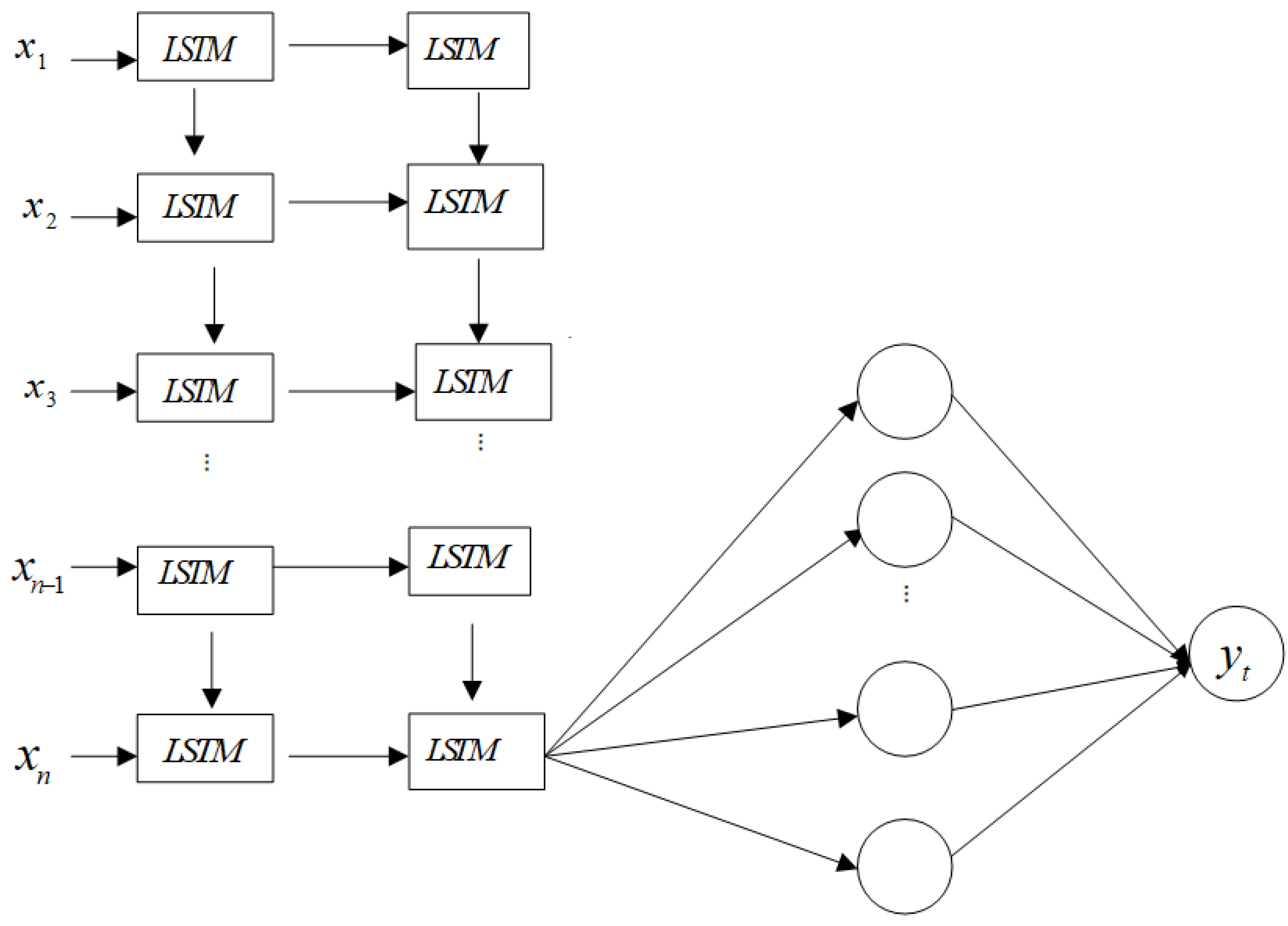
3.1.2. LSTM
3.1.3. ARMA
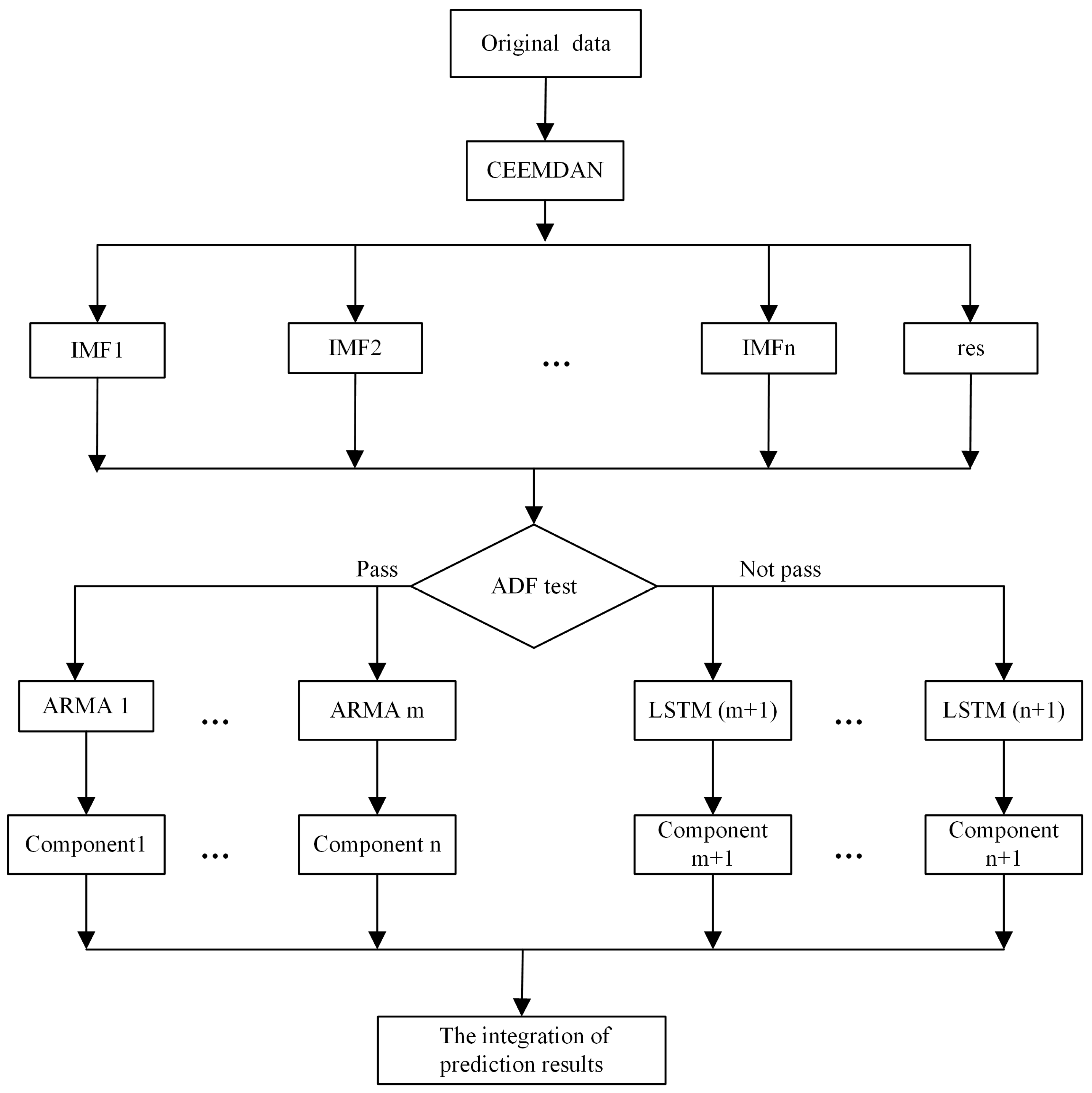
3.2. Proposed Model
- Given time series decomposition, using a CEEMDAN method (Equation (1)), time series data are decomposed into finite IMFs and residue. Components can be more or less volatile.
- Sequences with different stability are separated by an ADF stationary test (Equation (2)).
- The final result is the sum of the predictions of each component (Equation (5)).
4. Experimental Results and Discussions
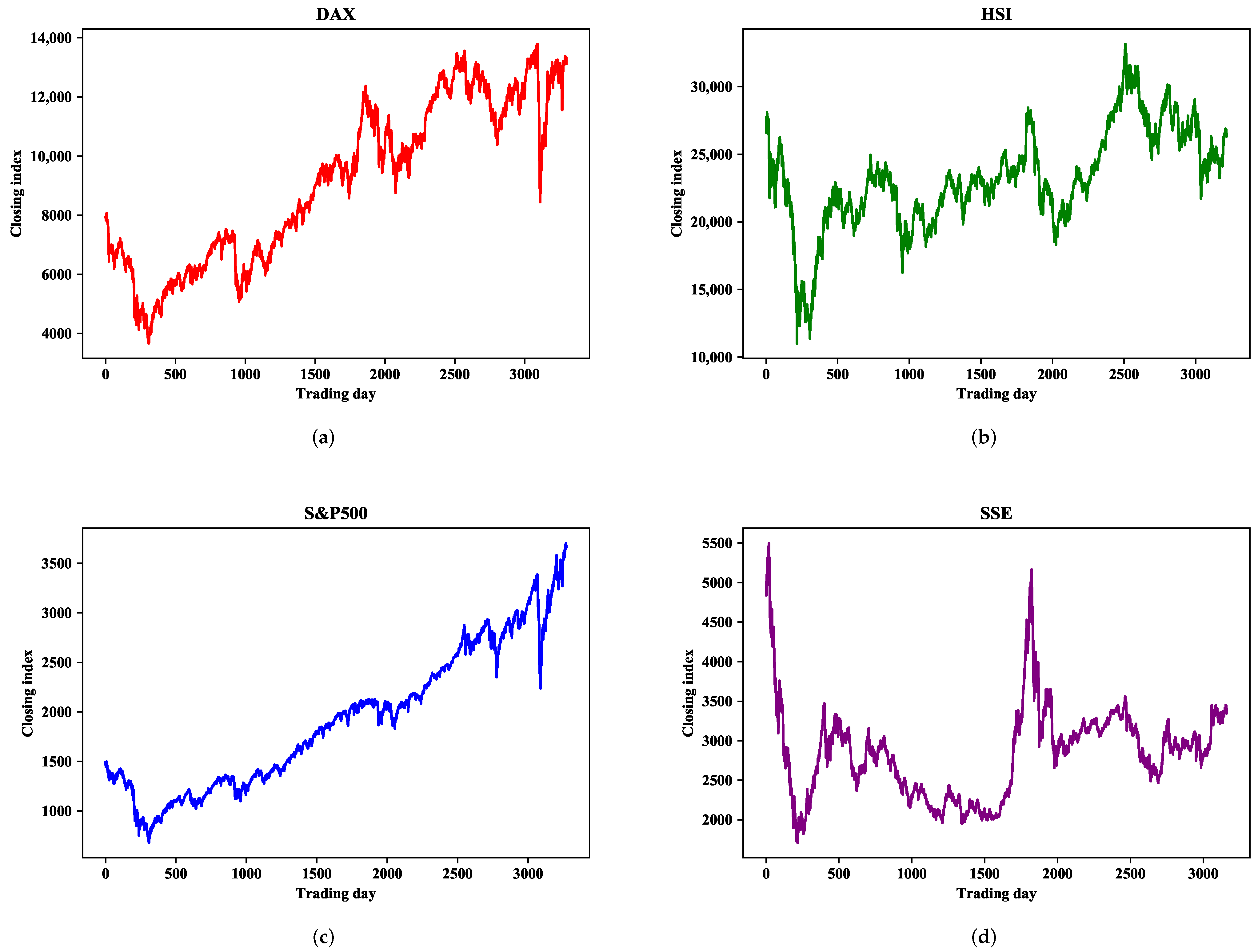
4.1. Datasets
4.2. Evaluation Metrics
4.3. Parameter Settings
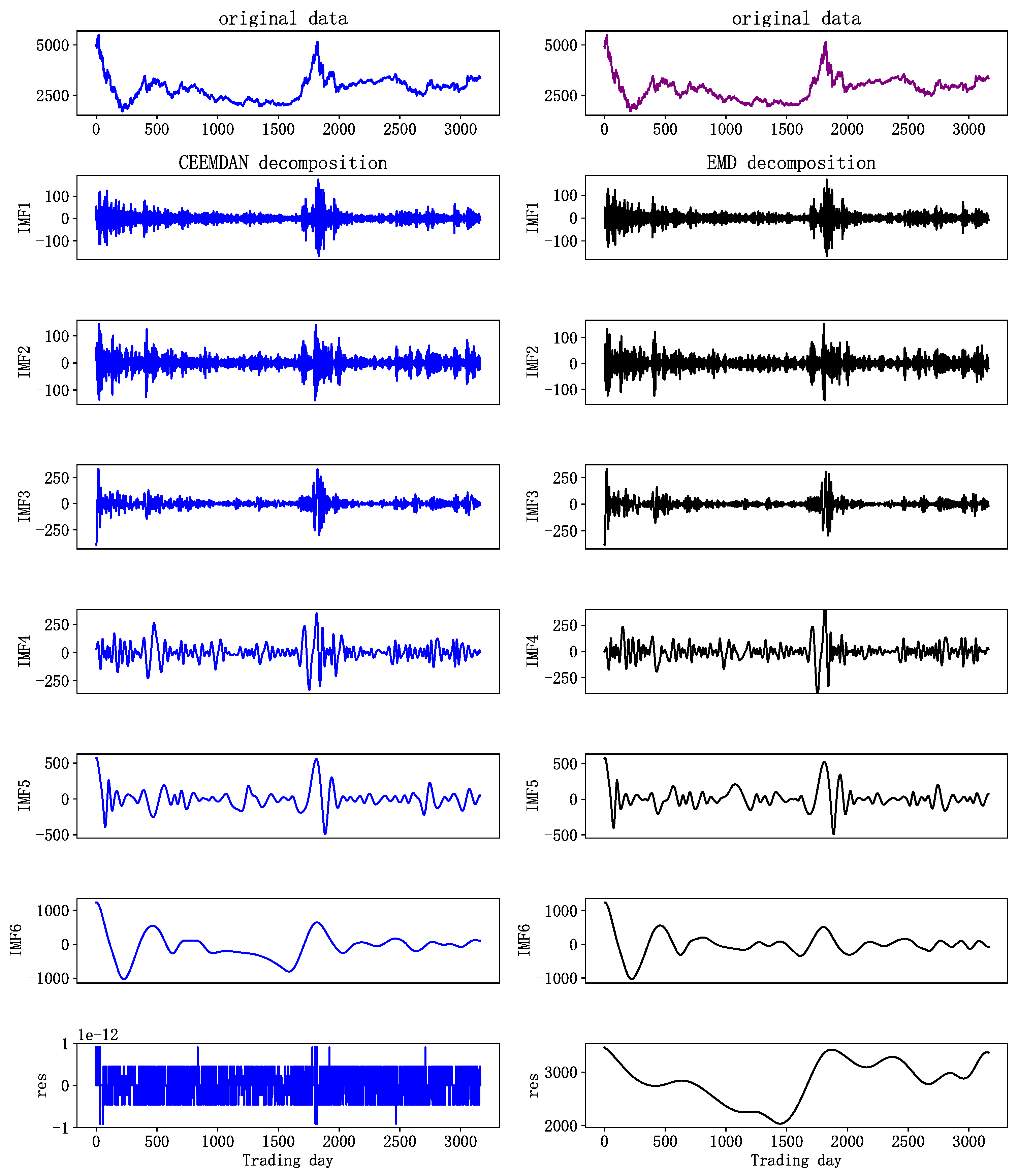
4.4. Decomposition Results of EMD and CEEMDAN
4.5. Comparative Models
- LSTM deep learning model: LSTM networks can automatically detect the best patterns suitable for raw data, and are widely utilized in financial time series modeling [23,24,25]. However, LSTM methods are susceptible to noise. The comparison result of CAL and LSTM can evaluate whether the proposed model can effectively improve the results of LSTM in complex time series modeling.
- Linear ARIMA model: ARIMA can better predict linear time series, but is not suitable for complex non-linear time series [4]. We combine ARMA and LSTM to extend the application range of the ARIMA time series model. In addition, the prediction effects of the ARIMA and CAL models are compared, which verifies the effectiveness of the proposed model compared with a single linear model.
- GRU: GRU is a simplified version of the LSTM. It uses only one state vector and two gate vectors, i.e., reset gate and update gate. The comparison result can evaluate whether the CAL model is better than other deep learning model.
- Bi-LSTM: To preserve the future and the past information, Bi-LSTM makes the neural network have the sequence information in both directions, i.e., backwards (future to past) and forward (past to future). The aim of the experiments is to show whether Bi-LSTM improves the prediction accuracy of LSTM. The experiments also verify the effectiveness of the proposed model compared with a single improved model.
- EMD-ARMA-LSTM model: EMD can generate more predictable components when fed into the decomposing module. CEEMDAN is designed to solve the problem of EMD mode mixing. To compare the prediction effects of EMD-ARMA-LSTM, and CAL, we verify the influence of different decomposition methods on model prediction.
- Hybrid ARIMA-ANN model [6]: ARIMA and ANN are adopted to model the linear and non-linear data [6], and empirical results demonstrate that ensemble models can effectively improve performance. We use the ARIMA-ANN model for comparison. The results can demonstrate the advantages of CAL over ARIMA-ANN when combining linear and non-linear models. The advantages of LSTM over an ANN in abstract feature extraction and prediction ability could also be verified.
- CEEMDAN-LSTM model [7]: The CEEMDAN-LSTM model integrates the advantages of CEEMDAN and LSTM but does not consider that the original time series may contain linearly correlated components, and the non-linear prediction of all decomposed sequences will affect the prediction performance of the model. The empirical results demonstrate the validity of the CAL model in comparison to the CEEMDAN-LSTM model.
4.6. Experiments and Discussions
- Statistics of MAE, RMSE, MAPE, and R are chosen to assess the consistency between predicted and observed terms. These indicators measure the deviation between forecast and reality from different aspects.
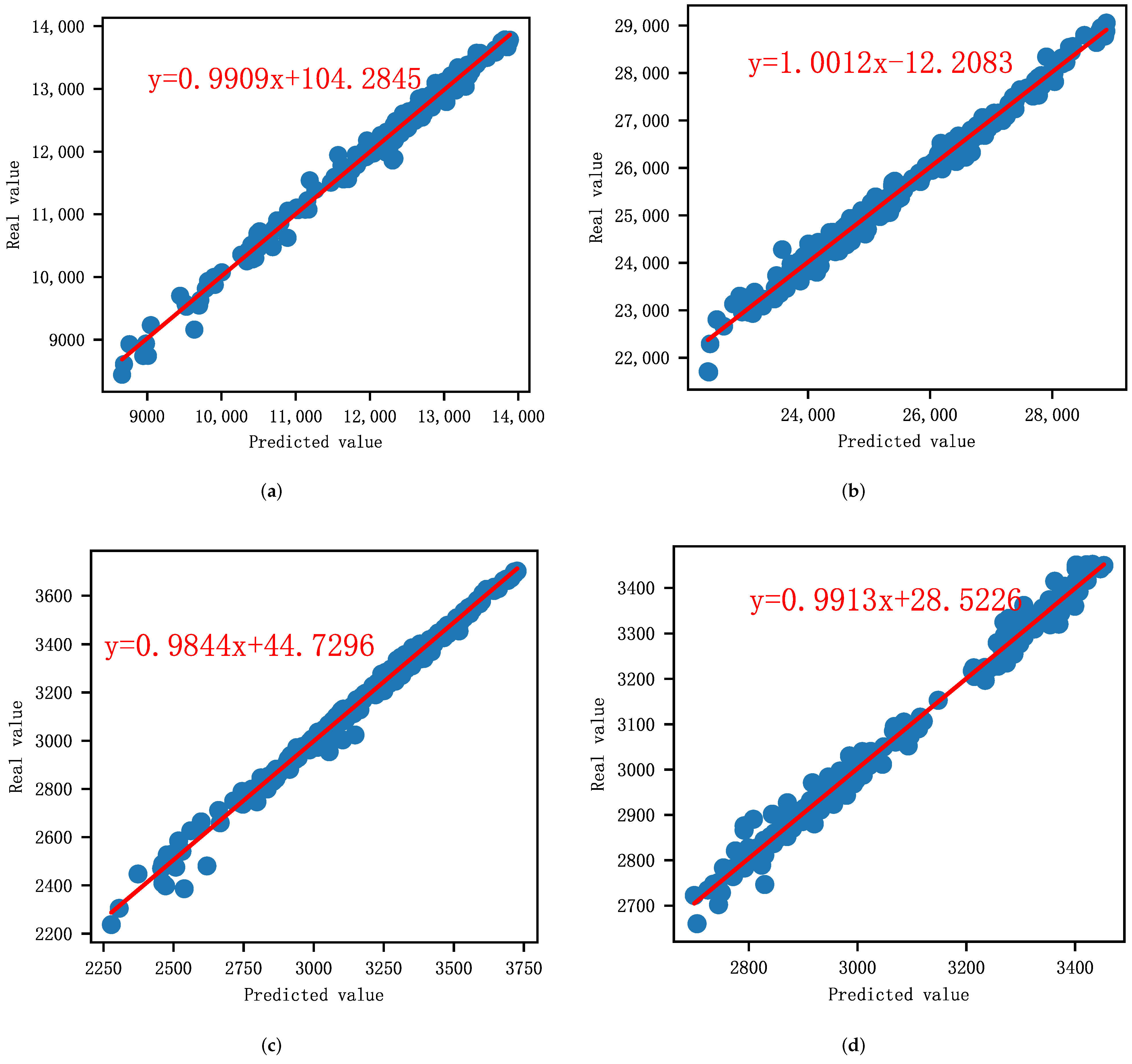
- A linear regression model is then used to further observe the performance of the CAL model; then, a series of technical diagnostics are leveraged to check the regression models.
4.6.1. Observation of the Statistical Data
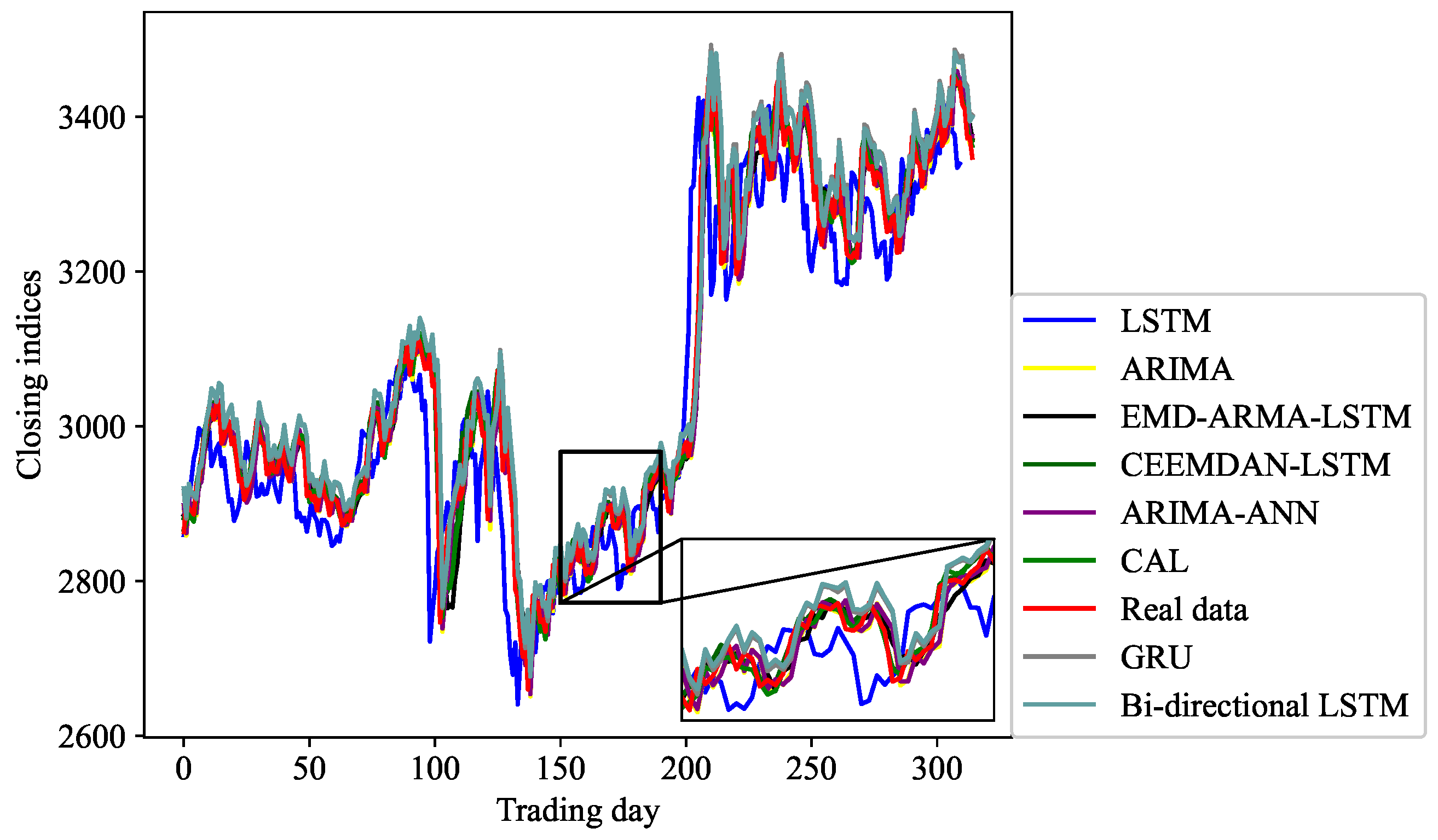
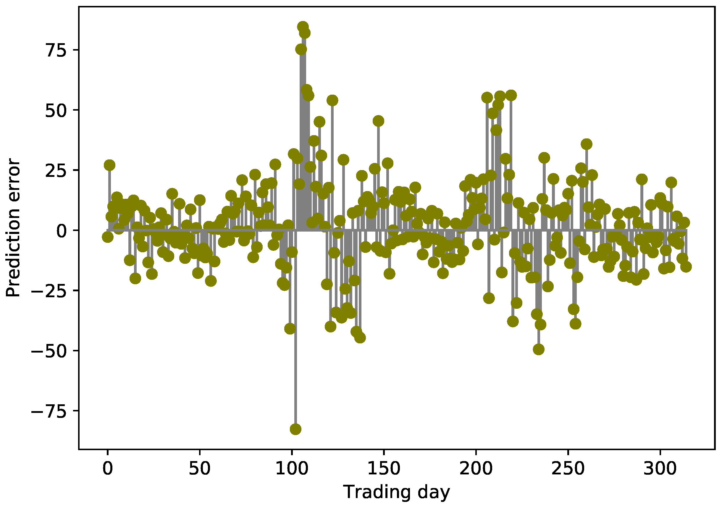
4.6.2. Prediction Results and Errors
4.6.3. Regression Analysis
4.6.4. Summary
- Our proposed CAL model, with CEEMDAN-based methods, outperforms seven benchmark models in predictive accuracy on four stock indices from different developed stock markets, which indicates that methods with multi-scale decomposition can reduce the complexity of sequences, extract hidden features, and improve prediction accuracy.
- CAL can obtain predictions closer to real values than CEEMDAN-LSTM, which indicates that components after decomposition may have both linear and non-linear characteristics. Therefore, models combining ARMA and LSTM can obtain more accurate predictions than individual LSTM models.
- CAL can yield the closest prediction results in comparison to ARIMA-ANN. This indicates that the CAL model has advantages over some traditional hybrid models.
- The prediction results show that CAL has a smaller prediction error than EMD-ARMA-LSTM does, and this indicates that the CEEMDAN method is superior to EMD in data decomposition.
- In some volatile financial markets, a single prediction model, even improved deep learning model, has limited prediction ability because they cannot excavate internal movement rules of time series and reflect the multi-scale characteristics of financial time series.
- The linear regression analysis shows the strong correlation between the predicted values and the real values, and the proposed prediction model is effective.
5. Conclusions and Discussion
- Single data source analysis has certain limitations. Combined analysis with different data sources, such as text information [26], can improve prediction to a certain extent.
Author Contributions
Funding
Institutional Review Board Statement
Informed Consent Statement
Data Availability Statement
Conflicts of Interest
References
- Yan, B.; Aasma, M. A novel deep learning framework: Prediction and analysis of financial time series using CEEMD and LSTM. Expert Syst. Appl. 2020, 159, 113609. [Google Scholar]
- Zhou, F.; Zhou, H.M.; Yang, Z.; Yang, L. EMD2FNN: A strategy combining empirical mode decomposition and factorization machine based neural network for stock market trend prediction. Expert Syst. Appl. 2019, 115, 136–151. [Google Scholar] [CrossRef]
- Torres, M.E.; Colominas, M.A.; Schlotthauer, G.; Flandrin, P. A complete ensemble empirical mode decomposition with adaptive noise. In Proceedings of the 2011 IEEE International Conference on Acoustics, Speech and Signal Processing (ICASSP), Prague, Czech Republic, 22–27 May 2011; pp. 4144–4147. [Google Scholar]
- Büyükşahin, Ü.Ç.; Ertekin, Ş. Improving forecasting accuracy of time series data using a new ARIMA-ANN hybrid method and empirical mode decomposition. Neurocomputing 2019, 361, 151–163. [Google Scholar] [CrossRef] [Green Version]
- Wang, Z.; Lou, Y. Hydrological time series forecast model based on wavelet de-noising and ARIMA-LSTM. In Proceedings of the 2019 IEEE 3rd Information Technology, Networking, Electronic and Automation Control Conference (ITNEC), Chengdu, China, 15–17 March 2019; pp. 1697–1701. [Google Scholar]
- Babu, C.N.; Reddy, B.E. A moving-average filter based hybrid ARIMA–ANN model for forecasting time series data. Appl. Soft Comput. 2014, 23, 27–38. [Google Scholar] [CrossRef]
- Cao, J.; Li, Z.; Li, J. Financial time series forecasting model based on CEEMDAN and LSTM. Phys. Stat. Mech. Its Appl. 2019, 519, 127–139. [Google Scholar] [CrossRef]
- Khashei, M.; Bijari, M. A novel hybridization of artificial neural networks and ARIMA models for time series forecasting. Appl. Soft Comput. 2011, 11, 2664–2675. [Google Scholar] [CrossRef]
- Goodfellow, I.; Bengio, Y.; Courville, A. Deep Learning; MIT Press: Cambridge, MA, USA, 2016. [Google Scholar]
- Gers, F.A.; Eck, D.; Schmidhuber, J. Applying LSTM to time series predictable through time-window approaches. In Neural Nets WIRN Vietri-01; Springer: Berlin/Heidelberg, Germany, 2002; pp. 193–200. [Google Scholar]
- Bao, W.; Yue, J.; Rao, Y. A deep learning framework for financial time series using stacked autoencoders and long-short term memory. PLoS ONE 2017, 12, e0180944. [Google Scholar] [CrossRef] [Green Version]
- Chung, H.; Shin, K.S. Genetic algorithm-optimized long short-term memory network for stock market prediction. Sustainability 2018, 10, 3765. [Google Scholar] [CrossRef] [Green Version]
- Foster, W.; Collopy, F.; Ungar, L. Neural network forecasting of short, noisy time series. Comput. Chem. Eng. 1992, 16, 293–297. [Google Scholar] [CrossRef]
- Brace, M.C.; Schmidt, J.; Hadlin, M. Comparison of the forecasting accuracy of neural networks with other established techniques. In Proceedings of the First International Forum on Applications of Neural Networks to Power Systems, Seattle, WA, USA, 23–26 July 1991; pp. 31–35. [Google Scholar]
- Pai, P.F.; Lin, C.S. A hybrid ARIMA and support vector machines model in stock price forecasting. Omega 2005, 33, 497–505. [Google Scholar] [CrossRef]
- Kim, H.Y.; Won, C.H. Forecasting the volatility of stock price index: A hybrid model integrating LSTM with multiple GARCH-type models. Expert Syst. Appl. 2018, 103, 25–37. [Google Scholar] [CrossRef]
- Zhang, G.P. Time series forecasting using a hybrid ARIMA and neural network model. Neurocomputing 2003, 50, 159–175. [Google Scholar] [CrossRef]
- Kumar, M.; Thenmozhi, M. Forecasting stock index returns using ARIMA-SVM, ARIMA-ANN, and ARIMA-random forest hybrid models. Int. J. Bank. Account. Financ. 2014, 5, 284–308. [Google Scholar] [CrossRef]
- Huang, N.E.; Shen, Z.; Long, S.R.; Wu, M.C.; Shih, H.H.; Zheng, Q.; Yen, N.C.; Tung, C.C.; Liu, H.H. The empirical mode decomposition and the Hilbert spectrum for nonlinear and non-stationary time series analysis. Proc. R. Soc. London. Ser. Math. Phys. Eng. Sci. 1998, 454, 903–995. [Google Scholar] [CrossRef]
- Song, H.; Dai, J.; Luo, L.; Sheng, G.; Jiang, X. Power transformer operating state prediction method based on an LSTM network. Energies 2018, 11, 914. [Google Scholar] [CrossRef] [Green Version]
- Ren, B. The use of machine translation algorithm based on residual and LSTM neural network in translation teaching. PLoS ONE 2020, 15, e0240663. [Google Scholar] [CrossRef]
- Liu, M.D.; Ding, L.; Bai, Y.L. Application of hybrid model based on empirical mode decomposition, novel recurrent neural networks and the ARIMA to wind speed prediction. Energy Convers. Manag. 2021, 233, 113917. [Google Scholar] [CrossRef]
- Fischer, T.; Krauss, C. Deep learning with long short-term memory networks for financial market predictions. Eur. J. Oper. Res. 2018, 270, 654–669. [Google Scholar] [CrossRef] [Green Version]
- Petersen, N.C.; Rodrigues, F.; Pereira, F.C. Multi-output bus travel time prediction with convolutional LSTM neural network. Expert Syst. Appl. 2019, 120, 426–435. [Google Scholar] [CrossRef] [Green Version]
- Kim, T.Y.; Cho, S.B. Web traffic anomaly detection using C-LSTM neural networks. Expert Syst. Appl. 2018, 106, 66–76. [Google Scholar] [CrossRef]
- Hao, P.Y.; Kung, C.F.; Chang, C.Y.; Ou, J.B. Predicting stock price trends based on financial news articles and using a novel twin support vector machine with fuzzy hyperplane. Appl. Soft Comput. 2021, 98, 106806. [Google Scholar] [CrossRef]
- Wu, D.; Wang, X.; Wu, S. A Hybrid Method Based on Extreme Learning Machine and Wavelet Transform Denoising for Stock Prediction. Entropy 2021, 23, 440. [Google Scholar] [CrossRef] [PubMed]
- Yang, K.; Liu, Y.L.; Yao, Y.N.; Fan, S.D.; Mosleh, A. Operational time-series data modeling via LSTM network integrating principal component analysis based on human experience. J. Manuf. Syst. 2020, 61, 746–756. [Google Scholar] [CrossRef]
- Coyle, D.; Prasad, G.; McGinnity, T.M. Extracting features for a brain-computer interface by self-organising fuzzy neural network-based time series prediction. In Proceedings of the 26th Annual International Conference of the IEEE Engineering in Medicine and Biology Society, San Francisco, CA, USA, 1–5 September 2004; Volume 2, pp. 4371–4374. [Google Scholar]
- Wang, J.; Zhang, W.; Li, Y.; Wang, J.; Dang, Z. Forecasting wind speed using empirical mode decomposition and Elman neural network. Appl. Soft Comput. 2014, 23, 452–459. [Google Scholar] [CrossRef]


| Index | Count | Mean | Max | Min | Standard Deviation | ADF Test |
|---|---|---|---|---|---|---|
| DAX | 3300 | 9118.21 | 13,789.00 | 3666.41 | 2722.52 | 0.79 |
| HSI | 3219 | 23,206.70 | 33,154.12 | 11,015.84 | 3660.60 | 0.11 |
| S&P500 | 3273 | 1915.40 | 3702.25 | 676.53 | 713.03 | 0.99 |
| SSE | 3163 | 2846.43 | 5497.90 | 1706.70 | 586.51 | 0.01 |
| Parameter | Meaning | Value |
|---|---|---|
| Input layer | Number of input layer nodes | 128 |
| Hidden layer 1 | Number of first hidden layer nodes | 64 |
| Hidden layer 2 | Number of second hidden layer nodes | 16 |
| Output layer | Number of output layer nodes | 1 |
| Batch size | Pass through to the network at one time | 128 |
| Optimization algorithm | Select the training mode | Adam |
| Loss function | With the goal of minimizing the loss | MSE |
| Epochs | Number of training | 200 |
| Timesteps | Input time steps | 10 |
| Model | Comparison Purpose of Model Settings |
|---|---|
| LSTM | Comparison to single deep learning model |
| ARIMA | Comparison to single linear model |
| GRU | Comparison to other single non-linear model |
| Bi-LSTM | Comparison to improved deep learning model |
| EMD-ARMA-LSTM | Evaluation of CEEMDAN and EMD |
| ARIAM-ANN | Comparison of CAL to hybrid models [6] |
| CEEMDAN-LSTM | Comparison of CAL to stock forecasting model [7] |
| Model | MAE | RMSE | MAPE (%) | R |
|---|---|---|---|---|
| LSTM | 167.0816 | 224.5003 | 1.4006 | 0.9570 |
| ARIMA | 136.0422 | 206.5253 | 1.1633 | 0.9650 |
| GRU | 153.5215 | 216.7465 | 1.2982 | 0.9608 |
| Bi-LSTM LSTM | 138.0041 | 209.2315 | 1.1768 | 0.9641 |
| ARIMA-ANN | 140.4099 | 211.9800 | 1.1966 | 0.9630 |
| CEEMDAN-LSTM | 97.2277 | 128.2331 | 0.8106 | 0.9866 |
| EMD-ARMA-LSTM | 127.1255 | 191.0622 | 1.0771 | 0.9687 |
| CAL | 72.3340 | 101.8321 | 0.6099 | 0.9915 |
| Model | MAE | RMSE | MAPE (%) | R |
|---|---|---|---|---|
| LSTM | 257.7703 | 347.1944 | 1.0197 | 0.9454 |
| ARIMA | 250.9188 | 345.3399 | 0.995 | 0.9470 |
| GRU | 256.1635 | 345.9382 | 1.0134 | 0.9451 |
| Bi-LSTM | 258.2292 | 353.4523 | 1.0249 | 0.9450 |
| ARIMA-ANN | 249.1046 | 344.5775 | 0.9882 | 0.9469 |
| CEEMDAN-LSTM | 127.0750 | 168.3214 | 0.5023 | 0.9879 |
| EMD-ARMA-LSTM | 181.7516 | 235.1773 | 0.7187 | 0.9751 |
| CAL | 120.8184 | 159.8226 | 0.4789 | 0.9885 |
| Model | MAE | RMSE | MAPE (%) | R |
|---|---|---|---|---|
| LSTM | 33.4958 | 53.4345 | 1.1207 | 0.9595 |
| ARIMA | 34.1031 | 54.8336 | 1.1411 | 0.9598 |
| GRU | 43.3137 | 63.2251 | 1.4416 | 0.9469 |
| Bi-LSTM | 33.5198 | 53.4177 | 1.1262 | 0.9610 |
| ARIMA-ANN | 33.7170 | 53.6489 | 1.125 | 0.9608 |
| CEEMDAN-LSTM | 21.1496 | 30.1187 | 0.6964 | 0.9878 |
| EMD-ARMA-LSTM | 22.1886 | 33.4485 | 0.7334 | 0.9843 |
| CAL | 17.1362 | 26.1373 | 0.5645 | 0.9910 |
| Model | MAE | RMSE | MAPE (%) | R |
|---|---|---|---|---|
| LSTM | 38.3486 | 47.9563 | 1.2468 | 0.9475 |
| ARIMA | 25.1019 | 36.9815 | 0.819 | 0.9690 |
| GRU | 31.8217 | 43.1568 | 1.0355 | 0.9599 |
| Bi-LSTM | 31.8026 | 42.7439 | 1.0382 | 0.9596 |
| ARIMA-ANN | 25.6976 | 37.4014 | 0.8383 | 0.9686 |
| CEEMDAN-LSTM | 14.3562 | 19.6741 | 0.4681 | 0.9913 |
| EMD-ARMA-LSTM | 19.5074 | 28.5532 | 0.6382 | 0.9814 |
| CAL | 14.0294 | 19.9246 | 0.459 | 0.9911 |
| Model | Parameter | Estimation | SE | t | p |
|---|---|---|---|---|---|
| DAX | a | 0.9909 | 0.005 | 196.519 | 0.000 |
| b | 104.2845 | 62.836 | 1.660 | 0.098 | |
| HSI | a | 1.0012 | 0.006 | 167.616 | 0.000 |
| b | −12.2083 | 153.286 | −0.080 | 0.937 | |
| S&P500 | a | 0.9844 | 0.005 | 192.819 | 0.000 |
| b | 44.7296 | 16.195 | 2.762 | 0.006 | |
| SSE | a | 0.9913 | 0.005 | 187.342 | 0.000 |
| b | 28.5226 | 16.263 | 1.754 | 0.080 |
Publisher’s Note: MDPI stays neutral with regard to jurisdictional claims in published maps and institutional affiliations. |
© 2022 by the authors. Licensee MDPI, Basel, Switzerland. This article is an open access article distributed under the terms and conditions of the Creative Commons Attribution (CC BY) license (https://creativecommons.org/licenses/by/4.0/).
Share and Cite
Lv, P.; Wu, Q.; Xu, J.; Shu, Y. Stock Index Prediction Based on Time Series Decomposition and Hybrid Model. Entropy 2022, 24, 146. https://doi.org/10.3390/e24020146
Lv P, Wu Q, Xu J, Shu Y. Stock Index Prediction Based on Time Series Decomposition and Hybrid Model. Entropy. 2022; 24(2):146. https://doi.org/10.3390/e24020146
Chicago/Turabian StyleLv, Pin, Qinjuan Wu, Jia Xu, and Yating Shu. 2022. "Stock Index Prediction Based on Time Series Decomposition and Hybrid Model" Entropy 24, no. 2: 146. https://doi.org/10.3390/e24020146