Exact Solution of a Time-Dependent Quantum Harmonic Oscillator with Two Frequency Jumps via the Lewis–Riesenfeld Dynamical Invariant Method

Abstract

Harmonic oscillators with multiple abrupt jumps in their frequencies have been investigated by several authors during the last decades. We investigate the dynamics of a quantum harmonic oscillator with initial frequency ${\omega }_0$, which undergoes a sudden jump to a frequency ${\omega }_1$ and, after a certain time interval, suddenly returns to its initial frequency. Using the Lewis–Riesenfeld method of dynamical invariants, we present expressions for the mean energy value, the mean number of excitations, and the transition probabilities, considering the initial state different from the fundamental. We show that the mean energy of the oscillator, after the jumps, is equal or greater than the one before the jumps, even when ${\omega }_1<{\omega }_0$. We also show that, for particular values of the time interval between the jumps, the oscillator returns to the same initial state.

1. Introduction

The quantum harmonic oscillator potential with time-dependent parameters is relevant in modeling several problems in physics, and it has been investigated [1,2,3,4,5,6,7,8,9]. For example, the interaction between a spinless charged quantum particle and a time-dependent external classical electromagnetic field can be studied through a harmonic potential whose frequency depends explicitly on time [4,10,11,12,13], and this is used to model the quantum motion of this particle in a trap [14,15,16,17,18,19]. In the context of quantum electrodynamics, this potential is useful, for instance, to describe the free electromagnetic field in nonstationary media [8,9,20]. In the context of shortcuts to adiabaticity, time-dependent quantum oscillators have also been considered [21,22,23,24,25,26]. Other applications are found in relativistic quantum mechanics, quantum field theory, dynamical Casimir effect, and gravitation [27,28,29,30,31,32,33].

A particular case of a quantum harmonic oscillator with time-dependent parameters that shows sudden frequency jumps is investigated, for instance, in refs. [21,23,24,34,35,36,37,38,39,40,41]. Under such jumps (or any time dependence in the parameters), a classical oscillator in its ground state remains in the same state, whereas a quantum oscillator can become excited [35]. Moreover, the wave functions of quantum harmonic oscillators with time-dependent parameters describe squeezed states [5,9,42], For example, a sudden change in the oscillation frequency of ${}^{85}\mathrm{Rb}$ atoms in the vibrational fundamental state of a one-dimensional optical lattice generates squeezed states [43]. The description of squeezed states is relevant, for instance, in the implementation of schemes for noise minimization in quantum sensors, which increases their sensitivity (see, for instance, ref. [44] and references therein). Subtle points involving the squeezed states for the model of two frequency jumps were investigated, for instance, by Tibaduiza et al. in ref. [40], where the solution for this case was obtained via algebraic method.

In the present paper, we investigate the dynamics of a quantum harmonic oscillator with initial frequency ${\omega }_0$ that undergoes a sudden jump to a frequency ${\omega }_1$ and, after a certain time interval, suddenly returns to its initial frequency. Instead of using the algebraic method used in ref. [40], here, we use the Lewis–Riesenfeld (LR) method of dynamical invariants. The LR method [2,3,4] enables the calculation of the exact wave function of a system subjected, for instance, to a harmonic oscillator potential with time-dependent parameters, such as mass and frequency [5,42,45]. Using this method, we show that the results for the squeeze parameters, the quantum fluctuations of the position and momentum operators, and the probability amplitude of a transition from the fundamental state to an arbitrary energy eigenstate coincide with those found in ref. [40]. In addition, using the same LR method, we also obtain expressions for the mean energy value and for the mean number of excitations (which were not calculated in ref. [40]), as well as for the transition probabilities considering the initial state different from the fundamental (which generalizes the formula found in ref. [40]).

The paper is organized as follows. In Section 2.1, we review some results of the application of the LR method to the quantum harmonic oscillator with time-dependent frequency. In Section 2.2, we define the squeezing parameters and, from these and the oscillator wave function obtained via the LR method, we determine the quantum fluctuations of the position, momentum and Hamiltonian operators, the mean number of excitations, and the transition probabilities between different states. In Section 3, we apply the results of previous sections to the model of ref. [40] and analyze their physical implications. In Section 4, we present our final remarks.

2. Analytical Method

2.1. The Wave Function of the Harmonic Oscillator via Lewis–Riesenfeld Method

Let us consider the one-dimensional Schrödinger equation for a system whose Hamiltonian $\widehat{H}\left(t\right)$ explicitly depends on time [46,47,48],

$$\begin{array}{c}\hfill i\hslash \frac{\partial \Psi (x,t)}{\partial t}=\widehat{H}\left(t\right)\Psi (x,t).\end{array}$$

(1)

According to the LR method [2,3,4,5,9,42], given an invariant Hermitian operator $\widehat{I}\left(t\right)$ which satisfies

$$\begin{array}{c}\hfill \frac{\partial \widehat{I}\left(t\right)}{\partial t}+\frac{1}{i\hslash }\left[\widehat{I}\left(t\right),\widehat{H}\left(t\right)\right]=0,\end{array}$$

(2)

a particular solution ${\Psi }_n(x,t)$ of Equation (1) is

$$\begin{array}{c}\hfill {\Psi }_n(x,t)=exp\left[i{\alpha }_n\left(t\right)\right]{\Phi }_n(x,t),\end{array}$$

(3)

in which ${\Phi }_n(x,t)$ are the eigenfunctions of $\widehat{I}\left(t\right)$, found from

$$\begin{array}{c}\hfill \widehat{I}\left(t\right){\Phi }_n(x,t)={\lambda }_n{\Phi }_n(x,t),\end{array}$$

(4)

with ${\lambda }_n$ being time-independent eigenvalues of $\widehat{I}\left(t\right)$ and ${\alpha }_n\left(t\right)$ phase functions, obtained from the equation

$$\begin{array}{c}\hfill \frac{d{\alpha }_n\left(t\right)}{dt}={\int }_{-\infty }^{+\infty }dx{\Phi }_n^{*}(x,t)\left[i\frac{\partial }{\partial t}-\frac{1}{\hslash }\widehat{H}\left(t\right)\right]{\Phi }_n(x,t).\end{array}$$

(5)

The general solution $\Psi (x,t)$ of Equation (1) is

$$\Psi (x,t)=\sum _{n=0}^{\infty }{C}_n{\Psi }_n(x,t),$$

(6)

where the time-independent coefficients $C_n$ depend only on the initial conditions.

Specifically, for a time-dependent one-dimensional harmonic oscillator with mass $m_0$, whose time dependence is contained purely in its oscillation frequency $\omega \left(t\right)$, the Hamiltonian is given by

$$\begin{array}{c}\hfill \widehat{H}\left(t\right)=\frac{{\widehat{p}}^2}{2m_0}+\frac{1}{2}{m}_0\omega {\left(t\right)}^2{\widehat{x}}^2,\end{array}$$

(7)

where $\widehat{x}$ and $\widehat{p}$ are position and momentum operators, respectively, with $\left[\widehat{x},\widehat{p}\right]=i\hslash$. An operator $\widehat{I}\left(t\right)$ associated with Equation (7) is [4,5,9,42]

$$\begin{array}{c}\hfill \widehat{I}\left(t\right)=\frac{1}{2}\left\{{\left[\frac{\widehat{x}}{\rho \left(t\right)}\right]}^2+{\left[\rho \left(t\right)\widehat{p}-m_0\dot{\rho }\left(t\right)\widehat{x}\right]}^2\right\},\end{array}$$

(8)

wherein $\rho \left(t\right)$ is a real parameter which is the solution of the Ermakov–Pinney equation [49,50,51,52]

$$\begin{array}{c}\hfill \ddot{\rho }\left(t\right)+\omega {\left(t\right)}^2\rho \left(t\right)=\frac{1}{m_0^2\rho {\left(t\right)}^3}.\end{array}$$

(9)

The eigenfunctions of $\widehat{I}\left(t\right)$, given by Equation (8), are

$$\begin{array}{c}\hfill {\Phi }_n(x,t)=\frac{1}{\sqrt{2^{n}n!}}{\Phi }_0(x,t)H_n\left[\frac{x}{{\hslash }^{\frac{1}{2}}\rho \left(t\right)}\right],\end{array}$$

(10)

where $H_n$ are the Hermite polynomials of order n [53], ${\lambda }_n=\left(n+1/2\right)\hslash$, and

$$\begin{array}{c}\hfill {\Phi }_0(x,t)={\left[\frac{1}{\pi \hslash \rho {\left(t\right)}^2}\right]}^{\frac{1}{4}}exp\left\{\frac{i{m}_0}{2\hslash }\left[\frac{\dot{\rho }\left(t\right)}{\rho \left(t\right)}+\frac{i}{m_0\rho {\left(t\right)}^2}\right]x^2\right\}.\end{array}$$

(11)

From Equation (5), the functions ${\alpha }_n\left(t\right)$ are given by

$$\begin{array}{c}\hfill {\alpha }_n\left(t\right)=-\frac{1}{m_0}\left(n+\frac{1}{2}\right){\int }_0^t\frac{d{t}^{\prime }}{\rho {\left(t^{\prime }\right)}^2}.\end{array}$$

(12)

Thus, from Equations (3), (10) and (12), the wave function ${\Psi }_n(x,t)$ associated with the Hamiltonian (7) is

$$\begin{array}{c}\hfill {\Psi }_n(x,t)=\frac{1}{\sqrt{2^{n}n!}}exp\left[-\frac{i}{m_0}\left(n+\frac{1}{2}\right){\int }_0^t\frac{d{t}^{\prime }}{\rho {\left(t^{\prime }\right)}^2}\right]{\Phi }_0(x,t)H_n\left[\frac{x}{{\hslash }^{\frac{1}{2}}\rho \left(t\right)}\right].\end{array}$$

(13)

For the case in which the frequency is always constant ($\omega \left(t\right)={\omega }_0$), the solution of Equation (9) is $\rho \left(t\right)={\rho }_0$, where [4,6,42]

$$\begin{array}{c}\hfill {\rho }_0=\frac{1}{\sqrt{m_0{\omega }_0}}.\end{array}$$

(14)

Therefore, Equation (13) falls back to the wave function of a harmonic oscillator with time-independent mass and frequency, ${\Psi }_n^{\left(0\right)}(x,t)$, given by [46,47,48]

$$\begin{array}{c}\hfill {\Psi }_n^{\left(0\right)}(x,t)=\frac{1}{\sqrt{2^{n}n!}}{\left(\frac{m_0{\omega }_0}{\pi \hslash }\right)}^{\frac{1}{4}}exp\left[-i\left(n+\frac{1}{2}\right){\omega }_{0}t-\frac{m_0{\omega }_0{x}^2}{2\hslash }\right]H_n\left[{\left(\frac{m_0{\omega }_0}{\hslash }\right)}^{\frac{1}{2}}x\right].\end{array}$$

(15)

2.2. Squeeze Parameters, Quantum Fluctuations, Mean Number of Excitations, and Transition Probability

As discussed in refs. [5,9,42,54], the quantum states of the time-dependent oscillator, characterized by the wave function ${\Psi }_n(x,t)$ (Equation (13)), are squeezed. Thus, we can define the squeeze parameter $r\left(t\right)$ and the squeeze phase $\varphi \left(t\right)$, which specify the squeezed state, in terms of the parameter $\rho \left(t\right)$ [55]:

$$\begin{array}{ccc}\hfill r\left(t\right)& =& {cosh}^{-1}\left\{{\left[\frac{m_0^2\dot{\rho }{\left(t\right)}^2+\rho {\left(t\right)}^{-2}+2m_0{\omega }_0+m_0^2{\omega }_0^2\rho {\left(t\right)}^2}{4m_0{\omega }_0}\right]}^{\frac{1}{2}}\right\},\hfill \end{array}$$

(16)

$$\begin{array}{ccc}\hfill \varphi \left(t\right)& =& {cos}^{-1}\left\{\frac{1+m_0{\omega }_0\rho {\left(t\right)}^2-2{cosh}^2\left[r\left(t\right)\right]}{2sinh\left[r\right(t\left)\right]cosh\left[r\right(t\left)\right]}\right\},\hfill \end{array}$$

(17)

with $r\left(t\right)\ge 0$ and $0\le \varphi \left(t\right)\le 2\pi$. From Equation (13), one can also obtain the expected value of a given observable $\widehat{O}\left(t\right)$ in the state ${\Psi }_n(x,t)$ as

$$\begin{array}{c}\hfill \langle \widehat{O}\left(t\right)\rangle (n,t)={\int }_{-\infty }^{+\infty }dx{\Psi }_n^{*}(x,t)\widehat{O}\left(t\right){\Psi }_n(x,t),\end{array}$$

(18)

which, from Equations (16) and (17), can be written in terms of $r\left(t\right)$ and $\varphi \left(t\right)$. For the operators $\widehat{x}$ and $\widehat{p}$, one has [56]:

$$\begin{array}{c}\hfill \langle \widehat{x}\rangle (n,t)=\langle \widehat{p}\rangle (n,t)=0,\end{array}$$

(19)

$$\begin{array}{c}\hfill \langle {\widehat{x}}^2\rangle (n,t)=\left(n+\frac{1}{2}\right)\frac{\hslash }{m_0{\omega }_0}\{{cosh}^2\left[r\left(t\right)\right]+{sinh}^2\left[r\left(t\right)\right]+2sinh\left[r\left(t\right)\right]\\ \hfill \times cosh\left[r\left(t\right)\right]cos\left[\varphi \left(t\right)\right]\},\end{array}$$

(20)

$$\begin{array}{c}\hfill \langle {\widehat{p}}^2\rangle (n,t)=\left(n+\frac{1}{2}\right)m_0{\omega }_0\hslash \{{cosh}^2\left[r\left(t\right)\right]+{sinh}^2\left[r\left(t\right)\right]-2sinh\left[r\left(t\right)\right]\\ \hfill \times cosh\left[r\left(t\right)\right]cos\left[\varphi \left(t\right)\right]\},\end{array}$$

(21)

where it follows, from Equations (7), (20), and (21), that

$$\begin{array}{c}\hfill \langle \widehat{H}\left(t\right)\rangle (n,t)=\frac{\langle {\widehat{p}}^2\rangle (n,t)}{2m_0}+\frac{1}{2}{m}_0\omega {\left(t\right)}^2\langle {\widehat{x}}^2\rangle (n,t).\end{array}$$

(22)

From Equations (19)–(21), one finds the variances of the operators $\widehat{x}$:

$$\begin{array}{c}\hfill \langle {[\Delta \widehat{x}]}^2\rangle (n,t)=\langle {\widehat{x}}^2\rangle (n,t)-{\left[\langle \widehat{x}\rangle (n,t)\right]}^2,\end{array}$$

(23)

and $\widehat{p}$:

$$\begin{array}{c}\hfill \langle {[\Delta \widehat{p}]}^2\rangle (n,t)=\langle {\widehat{p}}^2\rangle (n,t)-{\left[\langle \widehat{p}\rangle (n,t)\right]}^2,\end{array}$$

(24)

which implies the uncertainty relationship

$$\begin{array}{c}\hfill \langle {[\Delta \widehat{x}]}^2\rangle (n,t)\langle {[\Delta \widehat{p}]}^2\rangle (n,t)\ge {\left(n+\frac{1}{2}\right)}^2{\hslash }^2\{{cosh}^4\left[r\left(t\right)\right]+{sinh}^4\left[r\left(t\right)\right]-2{sinh}^2\left[r\left(t\right)\right]\\ \hfill \times {cosh}^2\left[r\left(t\right)\right]cos\left[2\varphi \left(t\right)\right]\}.\end{array}$$

(25)

Due to the time dependence of the frequency, one can also determine the mean number of excitations $\langle \widehat{N}\rangle (n,t)$ that a system, subjected to this potential, can undergo. This is given by [57,58,59]

$$\begin{array}{c}\hfill \langle \widehat{N}\rangle (n,t)=n+\left(2n+1\right){sinh}^2\left[r\left(t\right)\right].\end{array}$$

(26)

For the fundamental state $n=0$, one finds $\langle \widehat{N}\rangle (0,t)={sinh}^2\left[r\left(t\right)\right]$, a result that agrees with refs. [33,56] for vacuum squeezed states. This means that a system, even in the fundamental state, could be excited due to the temporal variations in its frequency. The system subjected to the time-dependent harmonic potential can also make transitions between different states, since time-dependent potentials induce quantum systems to make transitions [46,47,48]. Let us consider that the system is initially at a stationary state ${\Psi }_m^{\left(0\right)}(x,t=0)$ with frequency ${\omega }_0$ and, due to a modification in its frequency from ${\omega }_0$ to $\omega \left(t\right)$, it evolves to a new state ${\Psi }_m(x,t)$ (Equation (13)). In this way, the probability to find the system in the state ${\Psi }_n^{\left(0\right)}(x,t)$ (Equation (15)), is given by [46,47,48]

$$\begin{array}{c}\hfill \mathcal{P}{\left(t\right)}_{m\to n}={\left|{\int }_{-\infty }^{+\infty }dx{\Psi }_n^{*\left(0\right)}(x,t){\Psi }_m(x,t)\right|}^2.\end{array}$$

(27)

Using Equations (13) and (15), one can find that $\mathcal{P}{\left(t\right)}_{m\to n}=0$ for odd values of $|n-m|$, and [57,60]

$$\begin{array}{c}\hfill \mathcal{P}{\left(t\right)}_{m\to n}=\frac{2^{m+n}min(m,n){!}^2{\left\{sinh\left[r\right(t\left)\right]\right\}}^{|n-m|}}{m!n!cosh\left[r\right(t\left)\right]}\\ \hfill \times {\left[\sum _{k=\frac{|n-m|}{2}}^{\frac{n+m}{2}}\frac{\left(\begin{array}{c}\frac{n+m}{2}\\ k\end{array}\right)\left(\begin{array}{c}\frac{n+m+2k-2}{4}\\ \frac{n+m}{2}\end{array}\right)k!}{\left(k-\frac{|n-m|}{2}\right)!{cosh}^k\left[r\left(t\right)\right]}\right]}^2,\end{array}$$

(28)

for even values of $|n-m|$, where $min(m,n)$ is the smallest value between m and n. Note that the fact that Equation (28) is nonzero only for even values of $|n-m|$ is related to the parity of the harmonic potential [61]. From Equations (26) (making $n=0$) and (28), we can relate the probability $\mathcal{P}{\left(t\right)}_{m\to n}$ to the mean number of excitations in the fundamental state $\langle \widehat{N}\rangle (0,t)$:

$$\begin{array}{c}\hfill \mathcal{P}{\left(t\right)}_{m\to n}=\frac{2^{m+n}min(m,n){!}^2{\left[\langle \widehat{N}\rangle (0,t)\right]}^{\frac{|n-m|}{2}}}{m!n!{\left[\langle \widehat{N}\rangle (0,t)+1\right]}^{\frac{1}{2}}}\\ \hfill \times {\left[\sum _{k=\frac{|n-m|}{2}}^{\frac{n+m}{2}}\frac{\left(\begin{array}{c}\frac{n+m}{2}\\ k\end{array}\right)\left(\begin{array}{c}\frac{n+m+2k-2}{4}\\ \frac{n+m}{2}\end{array}\right)k!}{\left(k-\frac{|n-m|}{2}\right)!{\left[\langle \widehat{N}\rangle (0,t)+1\right]}^{\frac{k}{2}}}\right]}^2.\end{array}$$

(29)

It follows that if the mean number of excitations in the fundamental state is nonzero, then the oscillator will have nonzero probabilities of making transitions between different energy levels. When we consider $m=n=0$ in Equation (28) (or in Equation (29)), one has the probability of persistence in the fundamental state, and, as a consequence, one can also obtain the probability of excitation, given by $1-\mathcal{P}{\left(t\right)}_{0\to 0}$ [40].

3. Oscillator with Two Frequency Jumps

Now, we apply the formulas shown in Section 2 to investigate the model discussed in ref. [40], namely an oscillator with

$$\begin{array}{c}\hfill \omega \left(t\right)=\left\{\begin{array}{cc}{\omega }_0,\hfill & t<0,\hfill \\ {\omega }_1,\hfill & 0<t<\tau ,\hfill \\ {\omega }_0,\hfill & t>\tau ,\hfill \end{array}\right.\end{array}$$

(30)

in which ${\omega }_0$ and ${\omega }_1$ are constant frequencies, and $\tau$ is the length of the time interval between the frequency jumps.

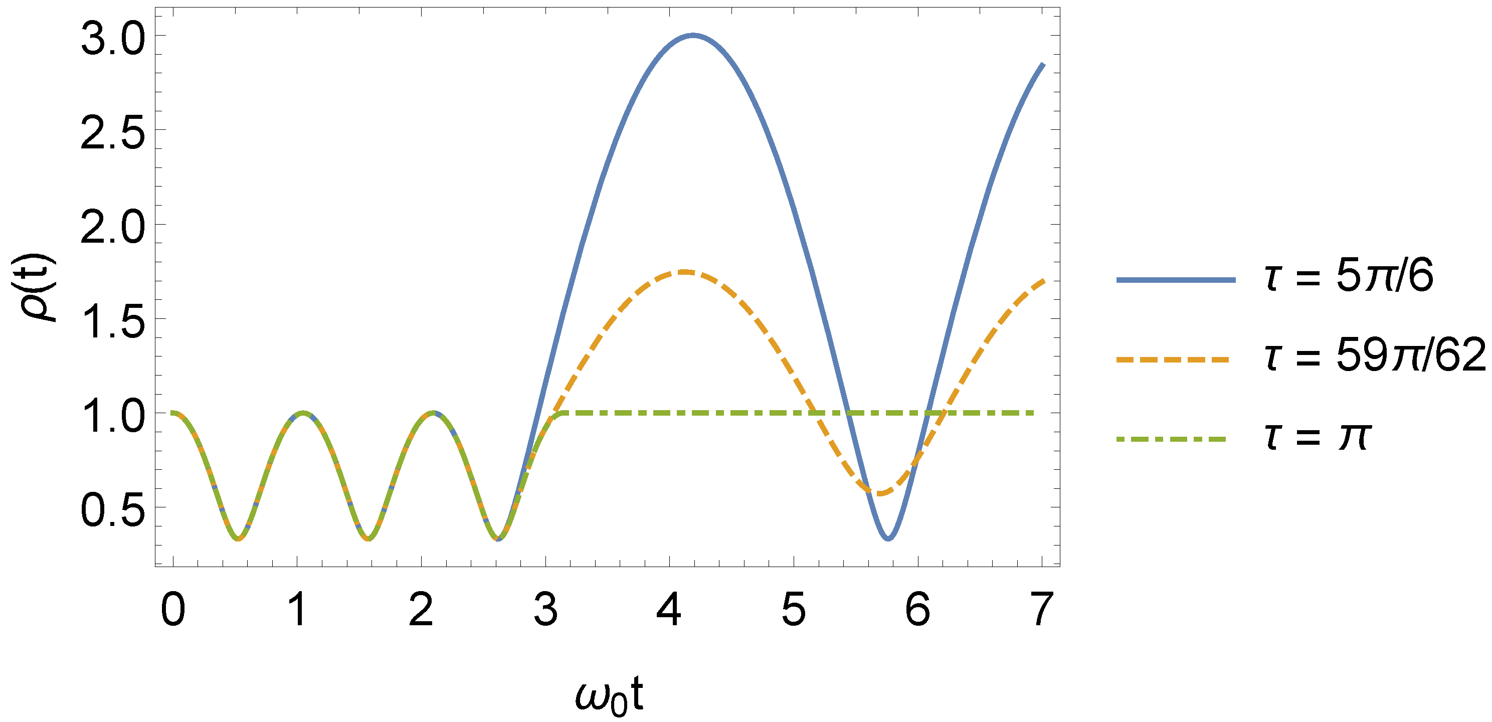
3.1. Solution and General Behavior of the $\rho \left(t\right)$ Parameter

Due to the form of Equation (30), the $\rho \left(t\right)$ parameter can be written as

$$\begin{array}{c}\hfill \rho \left(t\right)=\left\{\begin{array}{cc}{\rho }_0,\hfill & t<0,\hfill \\ {\rho }_1\left(t\right),\hfill & 0<t<\tau ,\hfill \\ {\rho }_2\left(t\right),\hfill & t>\tau ,\hfill \end{array}\right.\end{array}$$

(31)

where ${\rho }_0$ is given in Equation (14), and ${\rho }_1\left(t\right)$ and ${\rho }_2\left(t\right)$ are calculated next.

3.1.1. Interval $0<t<\tau$

For the interval $0<t<\tau$, the equation to be solved is

$$\begin{array}{c}\hfill {\ddot{\rho }}_1\left(t\right)+{\omega }_1^2{\rho }_1\left(t\right)=\frac{1}{m_0^2{\rho }_1{\left(t\right)}^3},\end{array}$$

(32)

with the conditions [6]

$$\begin{array}{c}\hfill {\rho }_1\left(t=0\right)=\frac{1}{\sqrt{m_0{\omega }_0}},{\dot{\rho }}_1\left(t=0\right)=0.\end{array}$$

(33)

The general solution for ${\rho }_1\left(t\right)$ is of the form [50,51]

$$\begin{array}{c}\hfill {\rho }_1\left(t\right)={\left[A_1{sin}^2\left({\omega }_{1}t\right)+B_1{cos}^2\left({\omega }_{1}t\right)+2C_{1}sin\left({\omega }_{1}t\right)cos\left({\omega }_{1}t\right)\right]}^{\frac{1}{2}},\end{array}$$

(34)

and the relationship between the constants $A_1$, $B_1$, and $C_1$ is

$$\begin{array}{c}\hfill A_1{B}_1-C_1^2=\frac{1}{m_0^2{\omega }_1^2}.\end{array}$$

(35)

Then, applying conditions (33) to Equation (34) and using relation (35), we obtain

$$\begin{array}{c}\hfill {\rho }_1\left(t\right)={\left[\frac{{\omega }_0{sin}^2\left({\omega }_{1}t\right)}{m_0{\omega }_1^2}+\frac{{cos}^2\left({\omega }_{1}t\right)}{m_0{\omega }_0}\right]}^{\frac{1}{2}}.\end{array}$$

(36)

3.1.2. Interval $t>\tau$

In the interval $t>\tau$, the Ermakov–Pinney equation has the form

$$\begin{array}{c}\hfill {\ddot{\rho }}_2\left(t\right)+{\omega }_0^2{\rho }_2\left(t\right)=\frac{1}{m_0^2{\rho }_2{\left(t\right)}^3}.\end{array}$$

(37)

The general solution of Equation (37) is

$$\begin{array}{c}\hfill {\rho }_2\left(t\right)={\left[A_2{sin}^2\left({\omega }_{0}t\right)+B_2{cos}^2\left({\omega }_{0}t\right)+2C_{2}sin\left({\omega }_{0}t\right)cos\left({\omega }_{0}t\right)\right]}^{\frac{1}{2}},\end{array}$$

(38)

with the constants $A_2$, $B_2$, and $C_2$ determined from the relationship

$$\begin{array}{c}\hfill A_2{B}_2-C_2^2=\frac{1}{m_0^2{\omega }_0^2},\end{array}$$

(39)

and the conditions for continuity

$$\begin{array}{c}\hfill {\rho }_1(t=\tau )={\rho }_2(t=\tau ),{\dot{\rho }}_1(t=\tau )={\dot{\rho }}_2(t=\tau ).\end{array}$$

(40)

Using Equations (36), (38), (39), and (40) results in

$$\begin{array}{c}\hfill A_2=\frac{1}{m_0{\omega }_0^3{\omega }_1^2}\{{\omega }_0^2{\omega }_1^2+\left[({\omega }_0^4-{\omega }_1^4){sin}^2\left({\omega }_0\tau \right)-{\omega }_0^2{\omega }_1^2+{\omega }_1^4\right]{sin}^2\left({\omega }_1\tau \right)\\ \hfill +2{\omega }_0{\omega }_1({\omega }_0-{\omega }_1)({\omega }_0+{\omega }_1)sin\left({\omega }_0\tau \right)cos\left({\omega }_0\tau \right)sin\left({\omega }_1\tau \right)cos\left({\omega }_1\tau \right)\},\end{array}$$

(41)

$$\begin{array}{c}\hfill B_2=\frac{1}{m_0{\omega }_0^3{\omega }_1^2}\{{\omega }_0^2{\omega }_1^2+\left[({\omega }_1^4-{\omega }_0^4){sin}^2\left({\omega }_0\tau \right)-{\omega }_0^2{\omega }_1^2+{\omega }_0^4\right]{sin}^2\left({\omega }_1\tau \right)\\ \hfill -2{\omega }_0{\omega }_1\left({\omega }_0-{\omega }_1\right)\left({\omega }_0+{\omega }_1\right)sin\left({\omega }_0\tau \right)cos\left({\omega }_0\tau \right)sin\left({\omega }_1\tau \right)cos\left({\omega }_1\tau \right)\},\end{array}$$

(42)

$$\begin{array}{c}\hfill C_2=\frac{1}{m_0{\omega }_0^3{\omega }_1^2}\{[({\omega }_0^2+{\omega }_1^2)sin\left({\omega }_0\tau \right)cos\left({\omega }_0\tau \right)sin\left({\omega }_1\tau \right)-2{\omega }_0{\omega }_1({sin}^2\left({\omega }_0\tau \right)\\ \hfill -1/2)cos\left({\omega }_1\tau \right)]\left({\omega }_0-{\omega }_1\right)\left({\omega }_0+{\omega }_1\right)sin\left({\omega }_1\tau \right)\}.\end{array}$$

(43)

3.1.3. General Behavior

The general solution for the $\rho \left(t\right)$ parameter is given by Equation (31), with ${\rho }_0$, ${\rho }_1\left(t\right)$ and ${\rho }_2\left(t\right)$ given by Equations (14), (36), (38), (41), (42), and (43). From these equations, it can be seen that the $\rho \left(t\right)$ parameter is a periodic function of time. Moreover, even when the frequency returns to its initial value ${\omega }_0$, this parameter will still, in general, be a periodic function of time. However, if we define ${\tau }_u=u\pi /{\omega }_1$ ($u>0$), and make $\tau ={\tau }_l$, where $l\in \mathbb{N}$, the $\rho \left(t\right)$ parameter returns to ${\rho }_0$ (Equation (14)), which means that although the oscillator feels the effect of the change in its frequency when it jumps from ${\omega }_0$ to ${\omega }_1$, if the frequency returns to ${\omega }_0$ at $\tau ={\tau }_l$, for $t>{\tau }_l$, the oscillator behaves as if nothing happened. In other words, if $\tau ={\tau }_l$, the abrupt change in the frequency is imperceptible to the oscillator when $t>{\tau }_l$. On the other hand, when $\tau ={\tau }_{l+1/2}$, the $\rho \left(t\right)$ parameter reaches its maximum value. The behavior of $\rho \left(t\right)$ is shown in Figure 1.

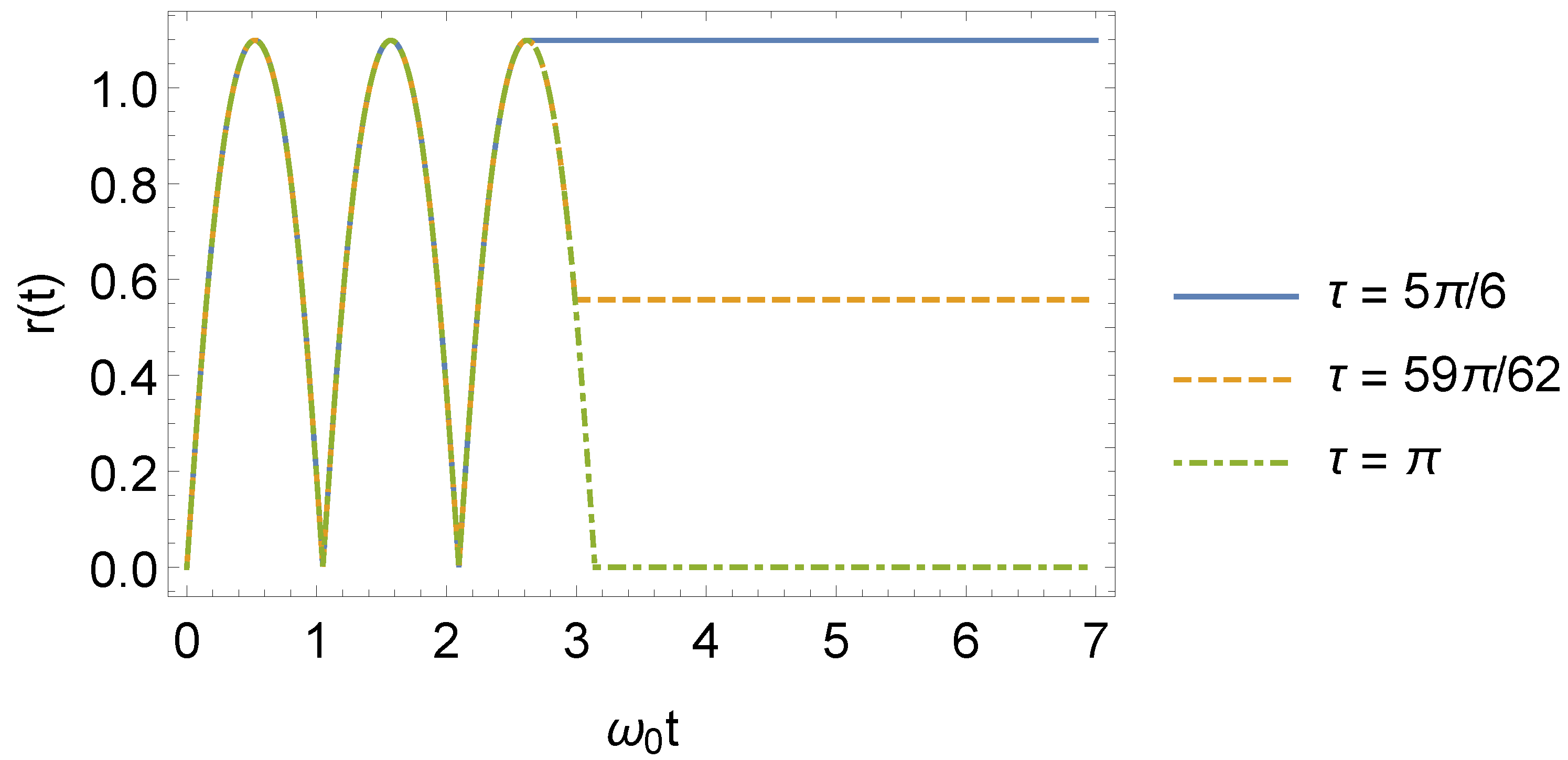
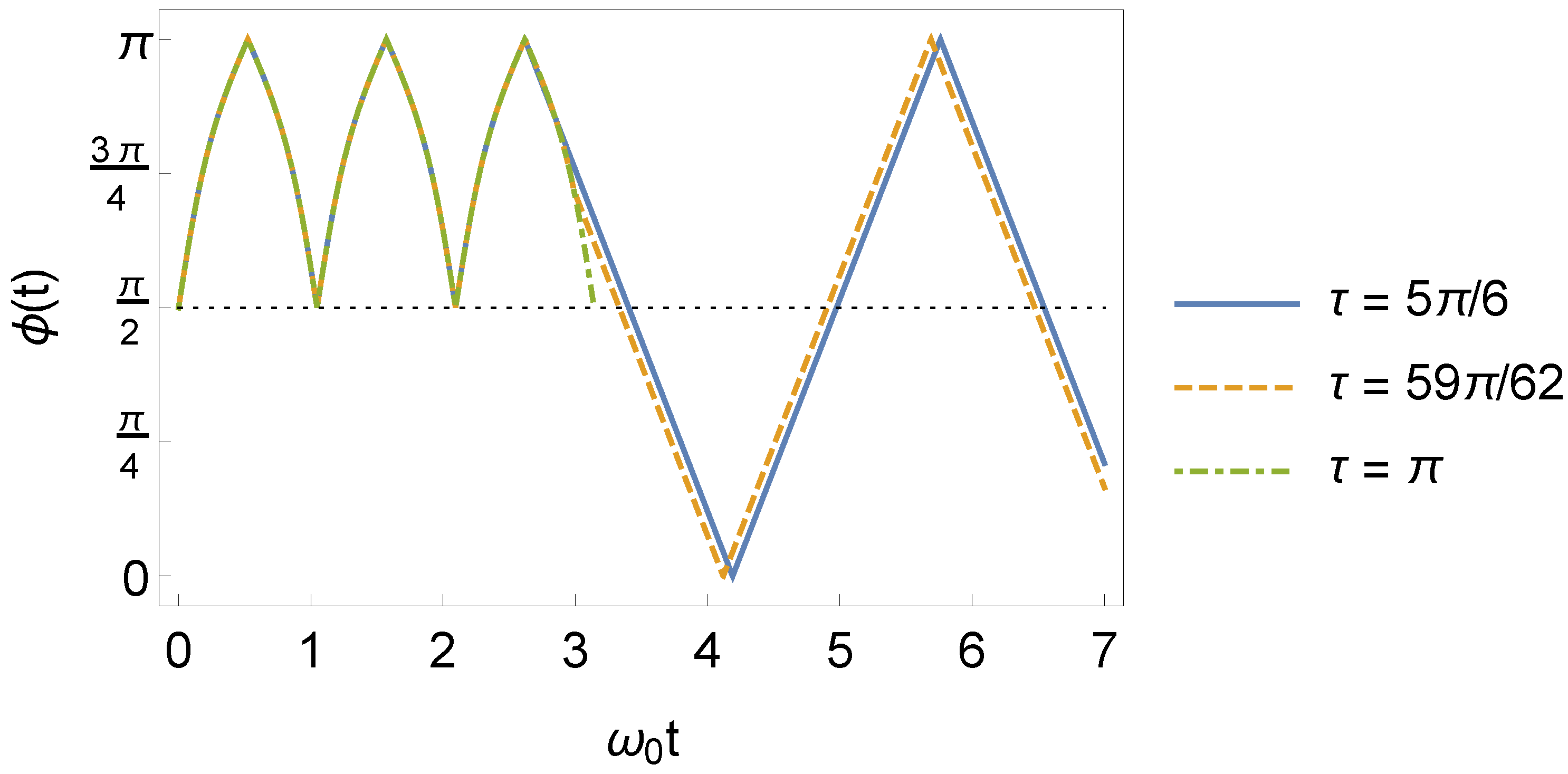
3.2. Squeeze Parameters

Because the frequency varies abruptly, squeezing occurs in the system [35,36,40]. Thus, now, we calculate the parameters $r\left(t\right)$ and $\varphi \left(t\right)$ associated with the model in Equation (30). We show that our results for these parameters agree with those found in ref. [40] via an exact algebraic method.

3.2.1. Parameter $r\left(t\right)$

The parameter $r\left(t\right)$ for any time interval is given by

$$\begin{array}{c}\hfill r\left(t\right)=\left\{\begin{array}{cc}0,\hfill & t<0,\hfill \\ r_1\left(t\right),\hfill & 0<t<\tau ,\hfill \\ r_2\left(t\right),\hfill & t>\tau .\hfill \end{array}\right.\end{array}$$

(44)

Note that $r(t<0)=0$ because the frequency of the oscillator is time-independent in this interval. Using Equation (36) in Equation (16), we obtain, for the interval $0<t<\tau$, the squeezing parameter $r_1\left(t\right)$, where

$$\begin{array}{c}\hfill r_1\left(t\right)={cosh}^{-1}\left\{\sqrt{1+{\left(\frac{{\omega }_1^2-{\omega }_0^2}{2{\omega }_0{\omega }_1}\right)}^2{sin}^2\left({\omega }_{1}t\right)}\right\},\end{array}$$

(45)

which is a result that agrees with the one found in ref. [40]. For the interval $t>\tau$, using Equation (38) in Equation (16), we find that $r_2\left(t\right)$, with

$$\begin{array}{c}\hfill r_2\left(t\right)=r_1\left(\tau \right),\end{array}$$

(46)

this also agrees with ref. [40]. Note that for $\tau ={\tau }_l$, one has $r_2\left(t\right)=0$. In Figure 2 (also found in ref. [40]), one can see the behavior of $r\left(t\right)$ for some values of $\tau$.

3.2.2. Parameter $\varphi \left(t\right)$

The squeeze phase $\varphi \left(t\right)$ for any time interval has the form

$$\begin{array}{c}\hfill \varphi \left(t\right)=\left\{\begin{array}{cc}\mathrm{undefined},\hfill & t<0,\hfill \\ {\varphi }_1\left(t\right),\hfill & 0<t<\tau ,\hfill \\ {\varphi }_2\left(t\right),\hfill & t>\tau ,\hfill \end{array}\right.\end{array}$$

(47)

where $\varphi \left(t\right)$ for $t<0$ is undefined because there is no squeeze in this interval. Using Equations (36) and (45) in Equation (17), we obtain that the squeeze phase for the interval $0<t<\tau$, ${\varphi }_1\left(t\right)$ is given by

$$\begin{array}{c}\hfill {\varphi }_1\left(t\right)={cos}^{-1}\left\{\frac{\left({\omega }_0^4-{\omega }_1^4\right){sin}^2\left({\omega }_{1}t\right)}{\sqrt{\left[4{\omega }_0^2{\omega }_1^2+{\left({\omega }_1^2-{\omega }_0^2\right)}^2{sin}^2\left({\omega }_{1}t\right)\right]{\left({\omega }_1^2-{\omega }_0^2\right)}^2{sin}^2\left({\omega }_{1}t\right)}}\right\},\end{array}$$

(48)

which also agrees with ref. [40]. To calculate the squeeze phase in the interval $t>\tau$, the reasoning is analogous, simply substituting Equations (38) and (46) into Equation (17).

From Figure 3, it can be seen that the squeezing phase will continue to vary in time, even for $t>\tau$.

Due of this time dependence, the fluctuations of the $\widehat{x}$ and $\widehat{p}$ operators will continue to depend on time in this interval, as we see later in Section 3.3 (see Equations (23) and (24)). Another point to be observed in Figure 3 concerns the behavior of the squeezing phase in the interval $t>\tau$, when $\tau ={\tau }_l$ (in the specific case of Figure 3, ${\tau }_l=\pi$). Since the squeeze parameter $r_2\left(t\right)$ (Equation (46)) is zero in this case, the system is no longer squeezed. Consequently, the squeeze phase is undefined for ${\tau }_l$. Therefore, its effect on the system will be negligible because there will be no more squeezing.

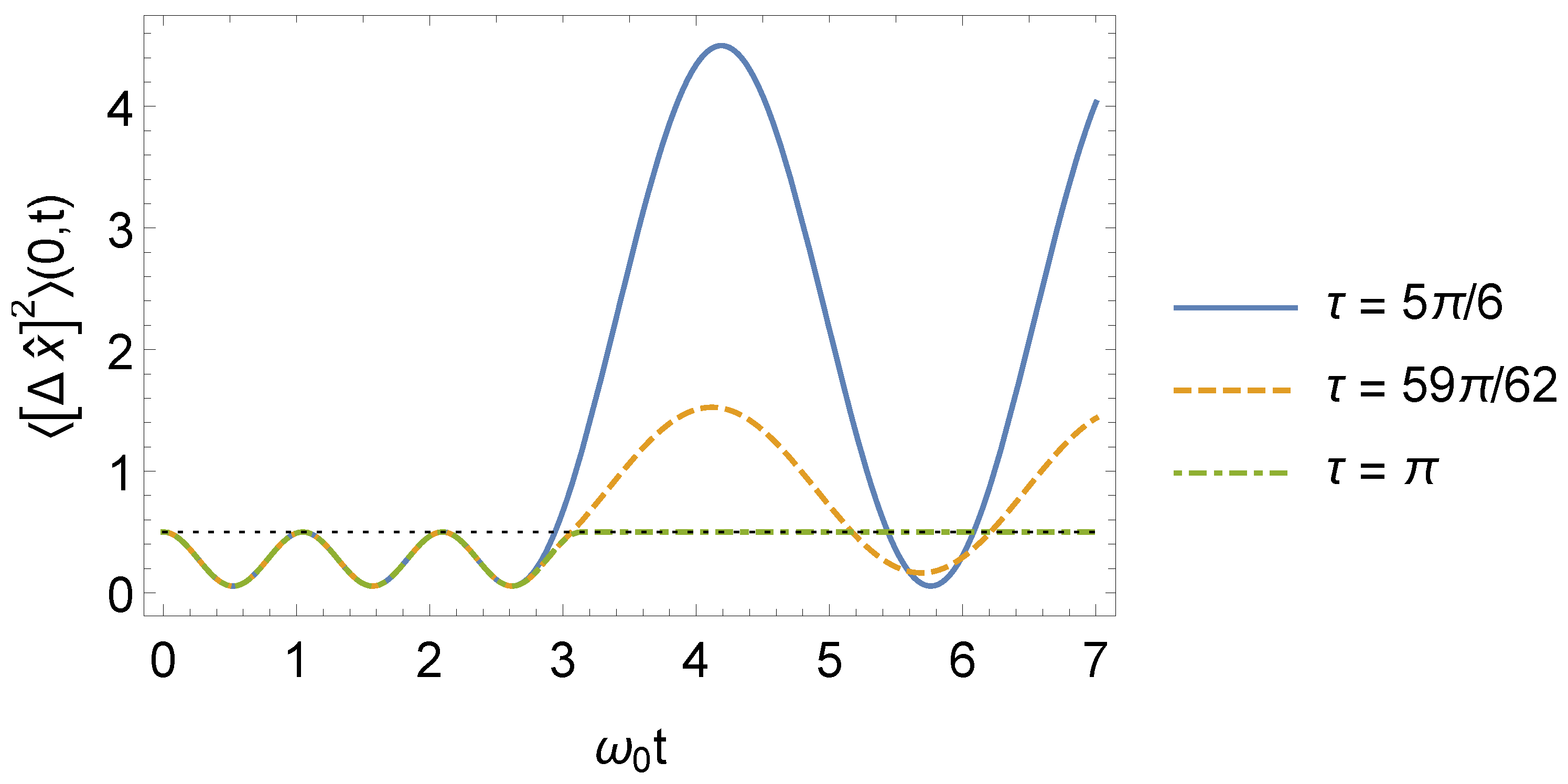
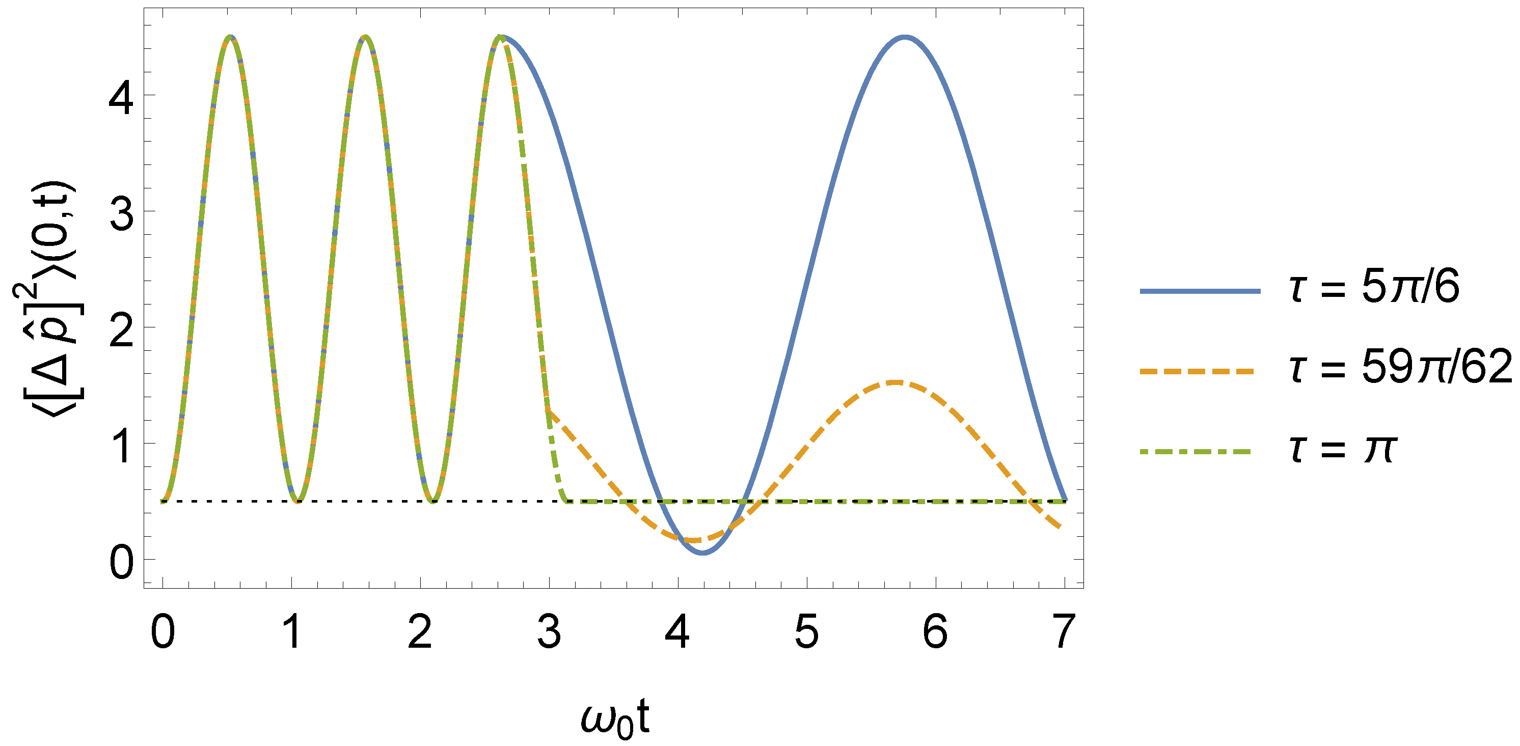
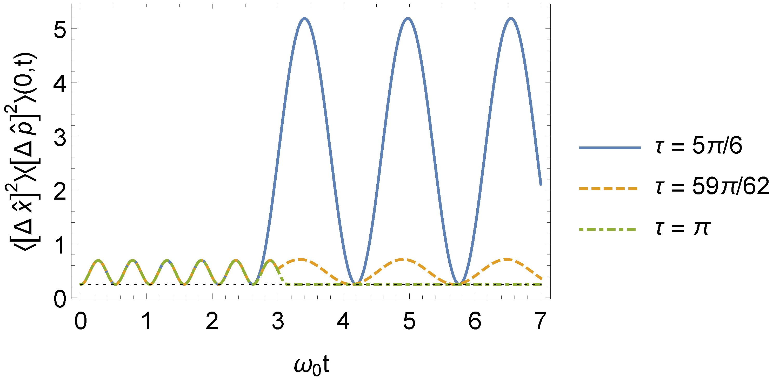
3.3. Quantum Fluctuations

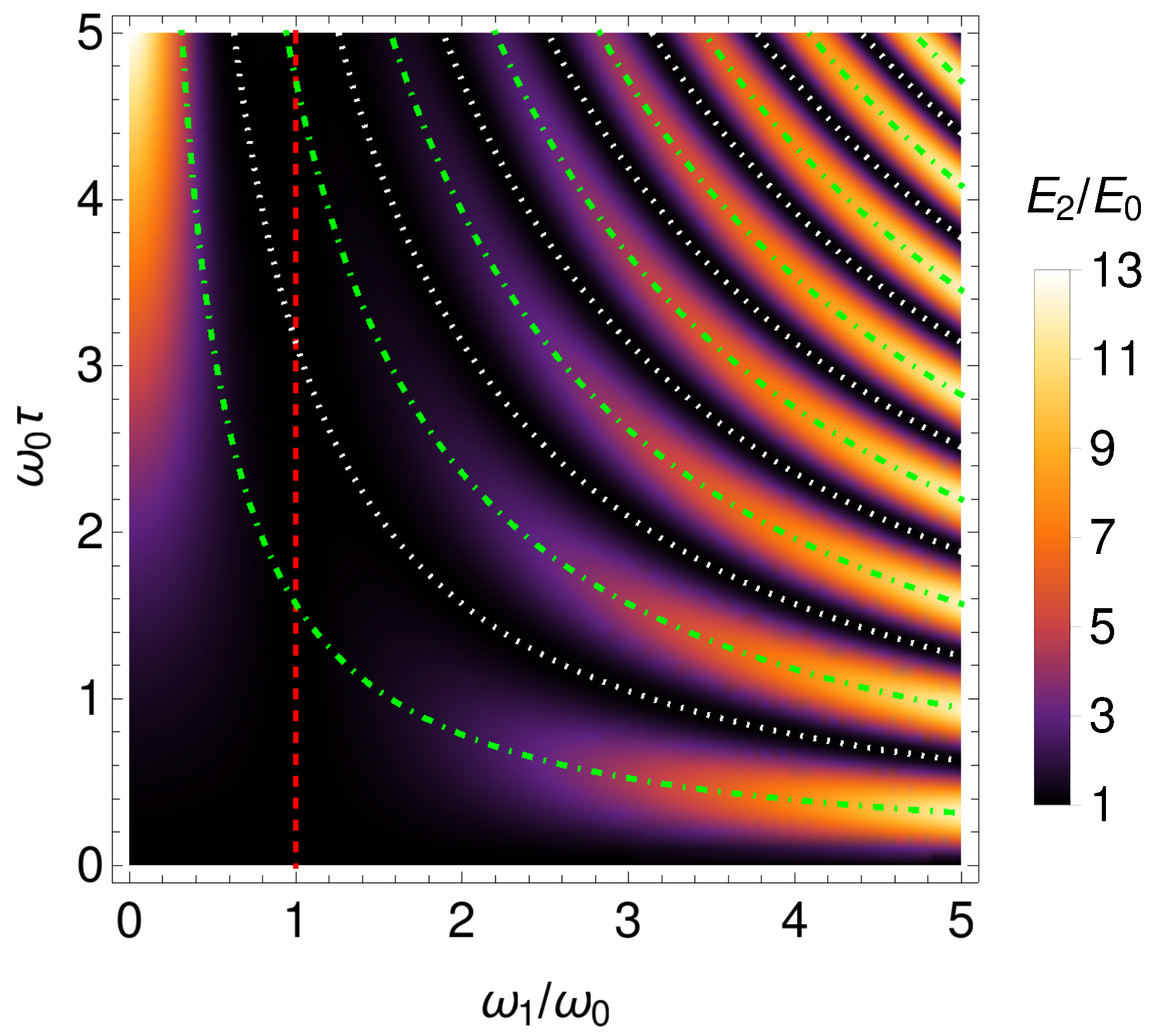
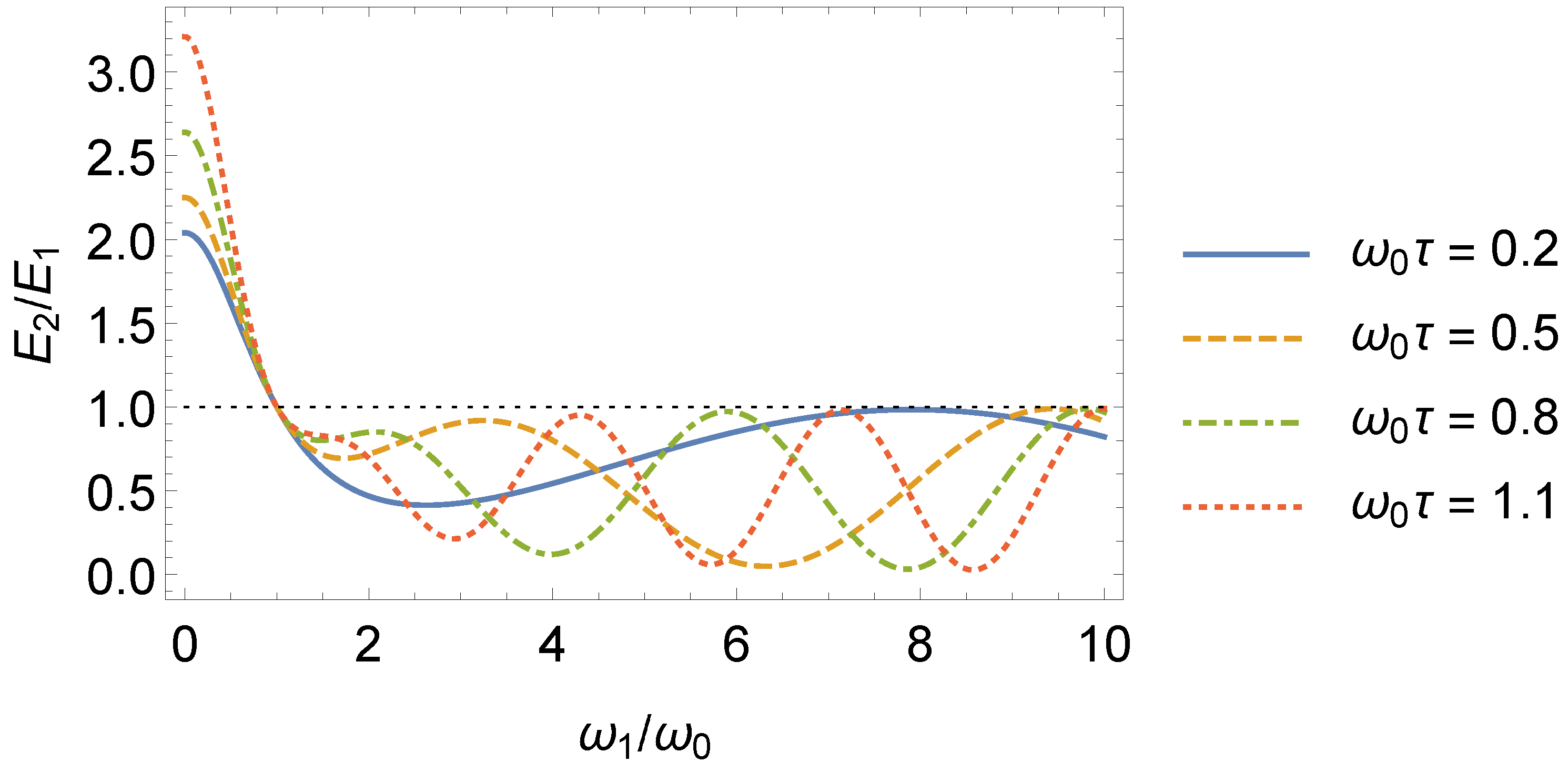
The variance of the $\widehat{x}$ operator for any time interval is given by

$$\begin{array}{c}\hfill \langle {[\Delta \widehat{x}]}^2\rangle (n,t)=\left\{\begin{array}{cc}\langle {[\Delta \widehat{x}]}_0^2\rangle \left(n\right),\hfill & t<0,\hfill \\ \langle {[\Delta \widehat{x}]}_1^2\rangle (n,t),\hfill & 0<t<\tau ,\hfill \\ \langle {[\Delta \widehat{x}]}_2^2\rangle (n,t),\hfill & t>\tau ,\hfill \end{array}\right.\end{array}$$

(49)

where [46]

$$\begin{array}{c}\hfill \langle {[\Delta \widehat{x}]}_0^2\rangle \left(n\right)=\left(n+\frac{1}{2}\right)\frac{\hslash }{m_0{\omega }_0}.\end{array}$$

(50)

Substituting Equations (45) and (48) into (23), we find, for the $\widehat{x}$ operator in the interval $0<t<\tau$,

$$\begin{array}{c}\hfill \langle {[\Delta \widehat{x}]}_1^2\rangle (n,t)=\left[\frac{{\omega }_0^2}{{\omega }_1^2}{sin}^2\left({\omega }_{1}t\right)+{cos}^2\left({\omega }_{1}t\right)\right]\langle {[\Delta \widehat{x}]}_0^2\rangle \left(n\right),\end{array}$$

(51)

which is in agreement with refs. [35,40]. For the interval $t>\tau$, the procedure is analogous, using Equations (16), (17), and (38) in Equation (23). In Figure 4, we show the behavior of $\langle {[\Delta \widehat{x}]}^2\rangle (n,t)$ for $n=0$.

Similarly, for the variance of the $\widehat{p}$ operator, we have

$$\begin{array}{c}\hfill \langle {[\Delta \widehat{p}]}^2\rangle (n,t)=\left\{\begin{array}{cc}\langle {[\Delta \widehat{p}]}_0^2\rangle \left(n\right),\hfill & t<0,\hfill \\ \langle {[\Delta \widehat{p}]}_1^2\rangle (n,t),\hfill & 0<t<\tau ,\hfill \\ \langle {[\Delta \widehat{p}]}_2^2\rangle (n,t),\hfill & t>\tau ,\hfill \end{array}\right.\end{array}$$

(52)

being [46]

$$\begin{array}{c}\hfill \langle {[\Delta \widehat{p}]}_0^2\rangle \left(n\right)=\left(n+\frac{1}{2}\right)\hslash m_0{\omega }_0.\end{array}$$

(53)

Through Equations (24), (45), and (48), we find, for the interval $0<t<\tau$, the expression [35,40]

$$\begin{array}{c}\hfill \langle {[\Delta \widehat{p}]}_1^2\rangle (n,t)=\left[\frac{{\omega }_1^2}{{\omega }_0^2}{sin}^2\left({\omega }_{1}t\right)+{cos}^2\left({\omega }_{1}t\right)\right]\langle {[\Delta \widehat{p}]}_0^2\rangle \left(n\right).\end{array}$$

(54)

To calculate the variance of the operator $\widehat{p}$ in the interval $t>\tau$, we must use Equations (16), (17), and (38) in Equation (24). The general behavior of $\langle {[\Delta \widehat{p}]}^2\rangle (n,t)$, when $n=0$, is schematized in Figure 5.

Thus, it is direct to see that the uncertainty relation between these operators in the interval $0<t<\tau$ has the form

$$\begin{array}{c}\hfill \langle {[\Delta \widehat{x}]}_1^2\rangle (n,t)\langle {[\Delta \widehat{p}]}_1^2\rangle (n,t)\ge \langle {[\Delta \widehat{x}]}_0^2\rangle \left(n\right)\langle {[\Delta \widehat{p}]}_0^2\rangle \left(n\right)\{1+[\left(\frac{{\omega }_1^2-{\omega }_0^2}{{\omega }_0{\omega }_1}\right)sin\left({\omega }_{1}t\right)\\ \hfill \times cos\left({\omega }_{1}t\right){{\displaystyle ]}}^2{\displaystyle \}},\end{array}$$

(55)

and the uncertainty relation for the interval $t>\tau$ is obtained in a similar way. Clearly, when ${\omega }_1={\omega }_0$, the uncertainty relation (Equation (55)) falls back to the uncertainty relation of a time-independent oscillator [46]. Furthermore, the uncertainty relation for an oscillator with time-independent frequency is also reobtained when $\tau ={\tau }_l$, as shown in Figure 6.

The results found by us (via the LR method) given in Equations (45), (46), (48), (51), and (54) are in agreement with those found in ref. [40]. Hereafter, we use the LR method to obtain new results concerning the model given in Equation (30).

3.4. Mean Energy

The expected value of the Hamiltonian operator is identified as the mean energy of the system, that is, $E\left(n,t\right)=\langle \widehat{H}\left(t\right)\rangle (n,t)$. The mean energy for the model in Equation (30) can be written as

$$\begin{array}{c}\hfill E(n,t)=\left\{\begin{array}{cc}{E}_0\left(n\right),\hfill & t<0,\hfill \\ E_1(n,t),\hfill & 0<t<\tau ,\hfill \\ E_2(n,t),\hfill & t>\tau ,\hfill \end{array}\right.\end{array}$$

(56)

wherein [46]

$$\begin{array}{c}\hfill E_0\left(n\right)=\left(n+\frac{1}{2}\right)\hslash {\omega }_0.\end{array}$$

(57)

For the interval $0<t<\tau$, through Equations (22), (51), (54), and (57), we find that the mean energy is time-independent, given by

$$\begin{array}{c}\hfill E_1(n,t)=\frac{1}{2}\left(1+\frac{{\omega }_1^2}{{\omega }_0^2}\right)E_0\left(n\right).\end{array}$$

(58)

When ${\omega }_1={\omega }_0$, Equation (58) reduces to $E_1(n,t)=E_0\left(n\right)$, as expected. Note that for ${\omega }_1/{\omega }_0<1$, $E_1(n,t)<E_0\left(n\right)$, whereas for ${\omega }_1/{\omega }_0>1$, we have $E_1(n,t)>E_0\left(n\right)$. When ${\omega }_1=0$, which means that the system is free in interval $0<t<\tau$, we have $E_1(n,t)=E_0\left(n\right)/2$. This can also be obtained by making ${\omega }_0\gg {\omega }_1$, which leads to $E_1(n,t)\approx E_0\left(n\right)/2$.

For the interval $t>\tau$, from Equations (16), (17), (22), (38), and (57), we have that the mean energy $E_2(n,t)$ is given by

$$\begin{array}{c}\hfill E_2(n,t)=\left[1+\frac{1}{2}{\left(\frac{{\omega }_1^2-{\omega }_0^2}{{\omega }_0{\omega }_1}\right)}^2{sin}^2\left({\omega }_1\tau \right)\right]E_0\left(n\right).\end{array}$$

(59)

Note that Equation (59) is independent of t, and $E_2(n,t)\ge E_0\left(n\right)$, even for ${\omega }_1<{\omega }_0$. The behavior of the ratio $E_2(n,t)/E_0\left(n\right)$ is illustrated in Figure 7.

For ${\omega }_1={\omega }_0$ (dashed line in Figure 7), Equation (59) recovers $E_2(n,t)=E_0\left(n\right)$, as expected. Furthermore, for $\tau ={\tau }_l$ (dotted lines in Figure 7), Equation (59) also gives $E_2(n,t)=E_0\left(n\right)$. In particular, the energy of this system is maximized when $\tau ={\tau }_{l+1/2}$ (dot–dashed lines in Figure 7). For ${\omega }_1/{\omega }_0\to 0$, we obtain $E_2(n,t)=\left(1+{\omega }_0^2{\tau }^2/2\right)E_0\left(n\right)$. Moreover, from Equations (46) and (59), we obtain

$$\begin{array}{c}\hfill E_2(n,t)=\left\{2{cosh}^2\left[r_2\left(t\right)\right]-1\right\}{E}_0\left(n\right).\end{array}$$

(60)

Thus, while there is squeeze, $E_2(n,t)>E_0\left(n\right)$. Therefore, the squeezing caused by the frequency jumps results in an increase in the mean energy of the oscillator with respect to its initial energy $E_0\left(n\right)$.

It is interesting to investigate the behavior of $E_2(n,t)/E_1(n,t)$. Unlike the ratio $E_2(n,t)/E_0\left(n\right)$, which is such that $E_2(n,t)/E_0\left(n\right)\ge 1$, the ratio $E_2(n,t)/E_1(n,t)$ can be lesser than, equal to, or greater than one, as shown in Figure 8. More specifically, for ${\omega }_1/{\omega }_0<1$, we have $E_2(n,t)/E_1(n,t)>1$, and when ${\omega }_1/{\omega }_0\to 0$, we find $E_2(n,t)=\left(2+{\omega }_0^2{\tau }^2\right)E_1(n,t)$. For ${\omega }_1/{\omega }_0>1$, the ratio $E_2(n,t)/E_1(n,t)$ oscillates between zero and one (see Figure 8). We highlight that, besides the trivial case ${\omega }_1={\omega }_0$, there are other values of the ratio ${\omega }_1/{\omega }_0$ that result in $E_2(n,t)=E_1(n,t)$.

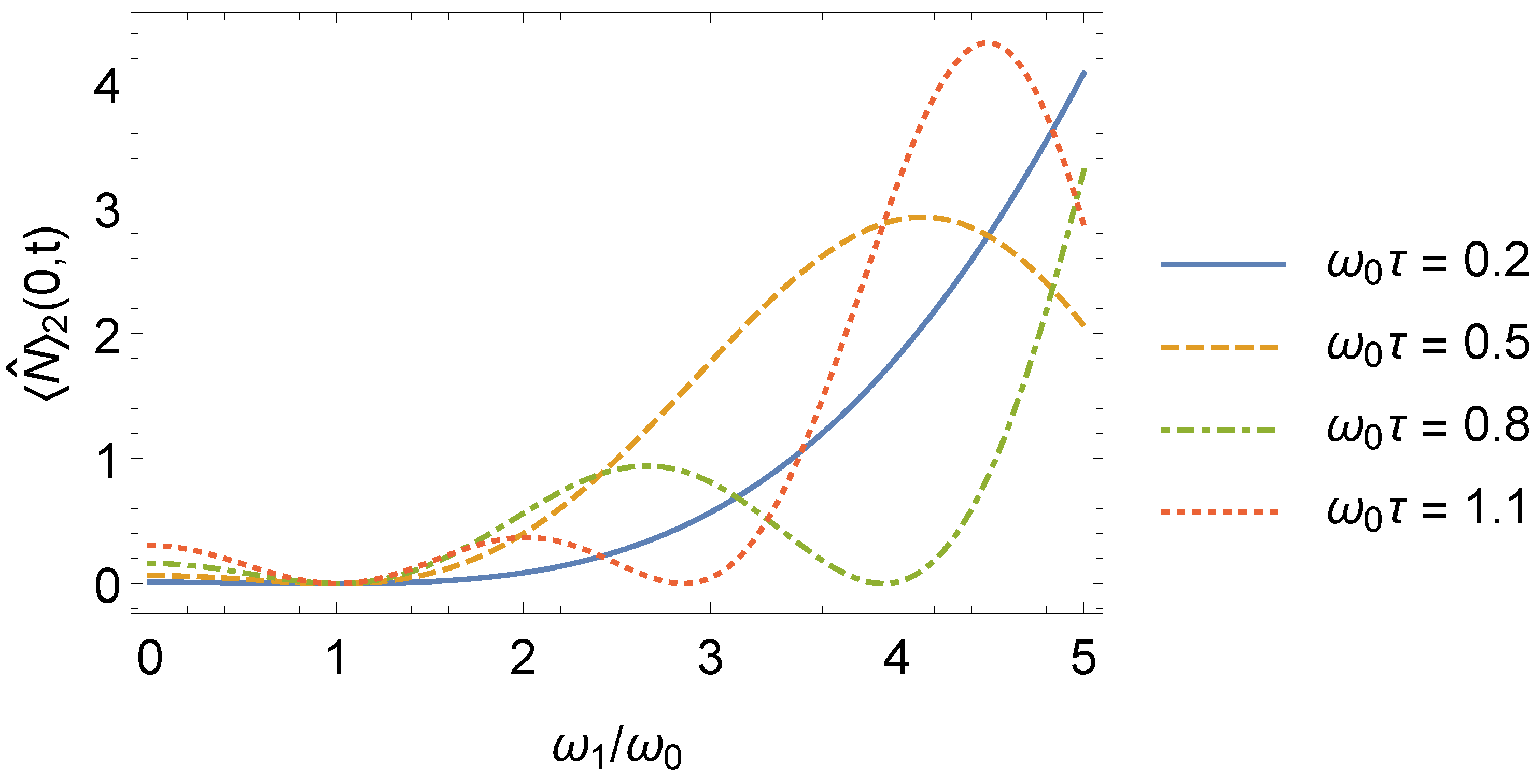
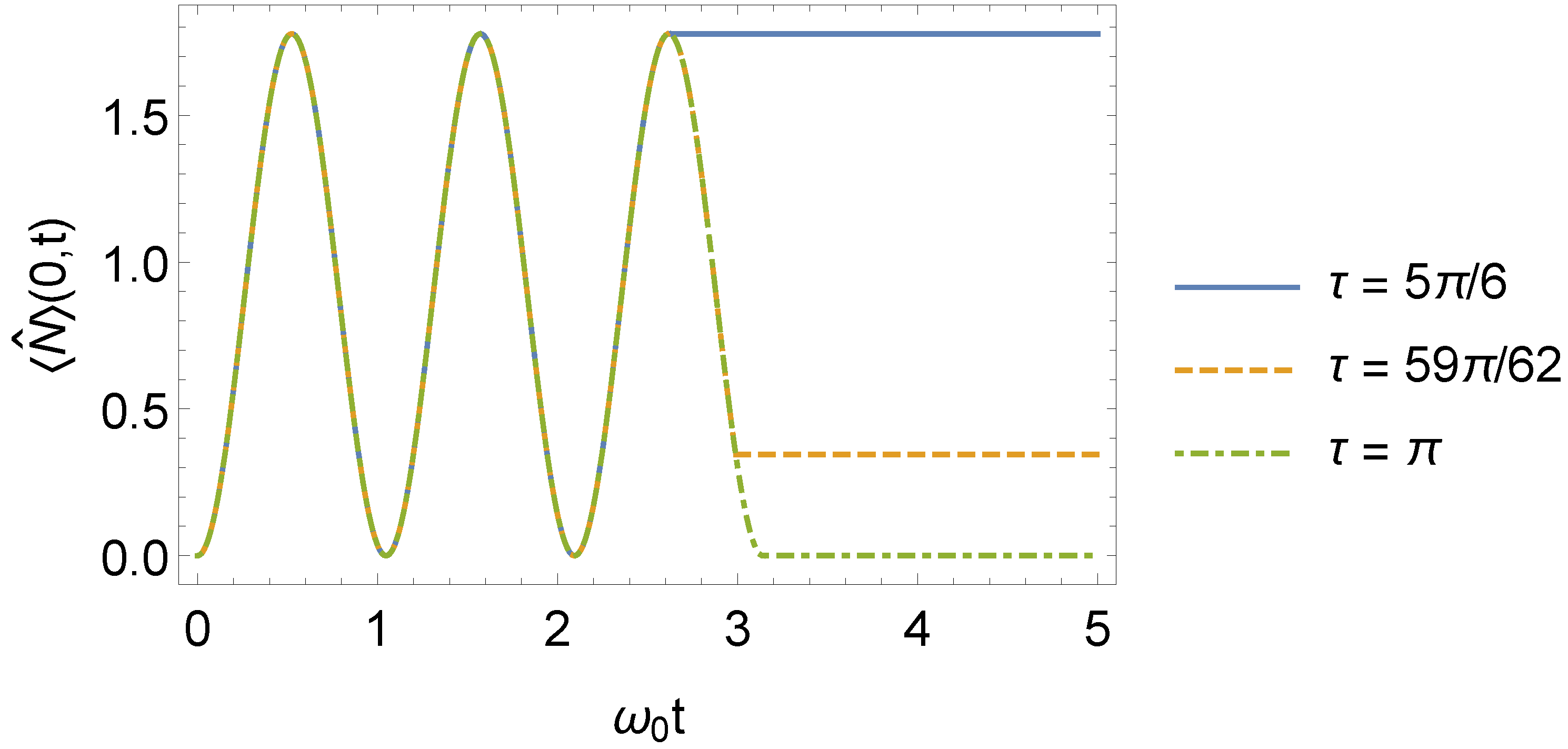
3.5. Mean Number of Excitations

The mean number of excitations, $\langle \widehat{N}\rangle (n,t)$, for the model in Equation (30), is given by

$$\begin{array}{c}\hfill \langle \widehat{N}\rangle (n,t)=\left\{\begin{array}{cc}{\langle \widehat{N}\rangle }_0\left(n\right),\hfill & t<0,\hfill \\ {\langle \widehat{N}\rangle }_1(n,t),\hfill & 0<t<\tau ,\hfill \\ {\langle \widehat{N}\rangle }_2(n,t),\hfill & t>\tau ,\hfill \end{array}\right.\end{array}$$

(61)

where [46]

$$\begin{array}{c}\hfill {\langle \widehat{N}\rangle }_0\left(n\right)=n.\end{array}$$

(62)

Given this, for the interval $0<t<\tau$, by means of Equations (26) and (45), we have

$$\begin{array}{c}\hfill {\langle \widehat{N}\rangle }_1(n,t)=n+\left(n+\frac{1}{2}\right)\left[\frac{1}{2}{\left(\frac{{\omega }_1^2-{\omega }_0^2}{{\omega }_0{\omega }_1}\right)}^2{sin}^2\left({\omega }_{1}t\right)\right].\end{array}$$

(63)

We remark the time dependence in ${\langle \widehat{N}\rangle }_1(n,t)$, whereas the mean energy in the interval $0<t<\tau$ (Equation (58)) is time-independent.

For the interval $t>\tau$, through Equations (26) and (46), we obtain ${\langle \widehat{N}\rangle }_2(n,t)$, given by

$$\begin{array}{c}\hfill {\langle \widehat{N}\rangle }_2(n,t)={\langle \widehat{N}\rangle }_1(n,\tau ).\end{array}$$

(64)

We also remark that for $\tau ={\tau }_l$, the behavior of the system returns to that of the time-independent oscillator found before the frequency jumps, i.e, ${\langle \widehat{N}\rangle }_2(n,t)={\langle \widehat{N}\rangle }_0\left(n\right)$. We highlight that there is excitation even for $n=0$, which means that, under jumps in its frequency, a quantum oscillator initially in its ground state can become excited (a classical oscillator in its ground state would remain in the same state). In addition, excitation can also occur when ${\omega }_1/{\omega }_0<1$, as shown in Figure 9.

Using Equations (59) and (64), we can also write $E_2(n,t)$ as

$$\begin{array}{c}\hfill E_2(n,t)=\left[{\langle \widehat{N}\rangle }_2(n,t)+\frac{1}{2}\right]\hslash {\omega }_0,\end{array}$$

(65)

which has the same structure as the expression for the energy eigenvalues of a time-independent oscillator (see Equation (57)). The time evolution of $\langle \widehat{N}\rangle (0,t)$, given by Equation (61) for $n=0$, is shown in Figure 10.

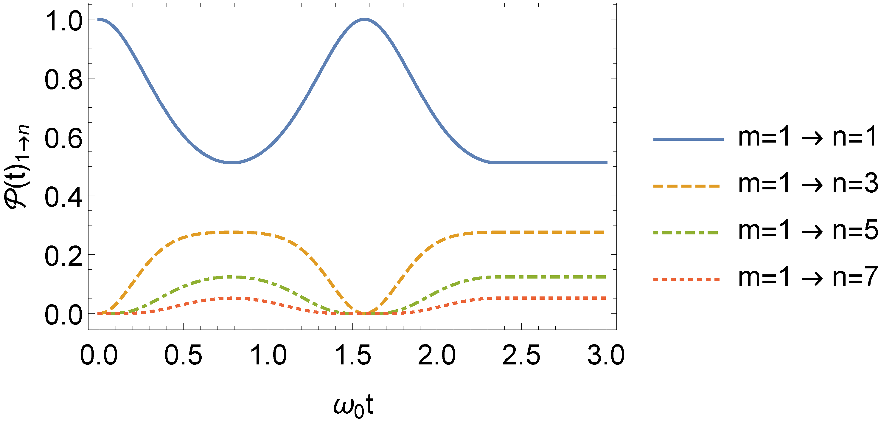
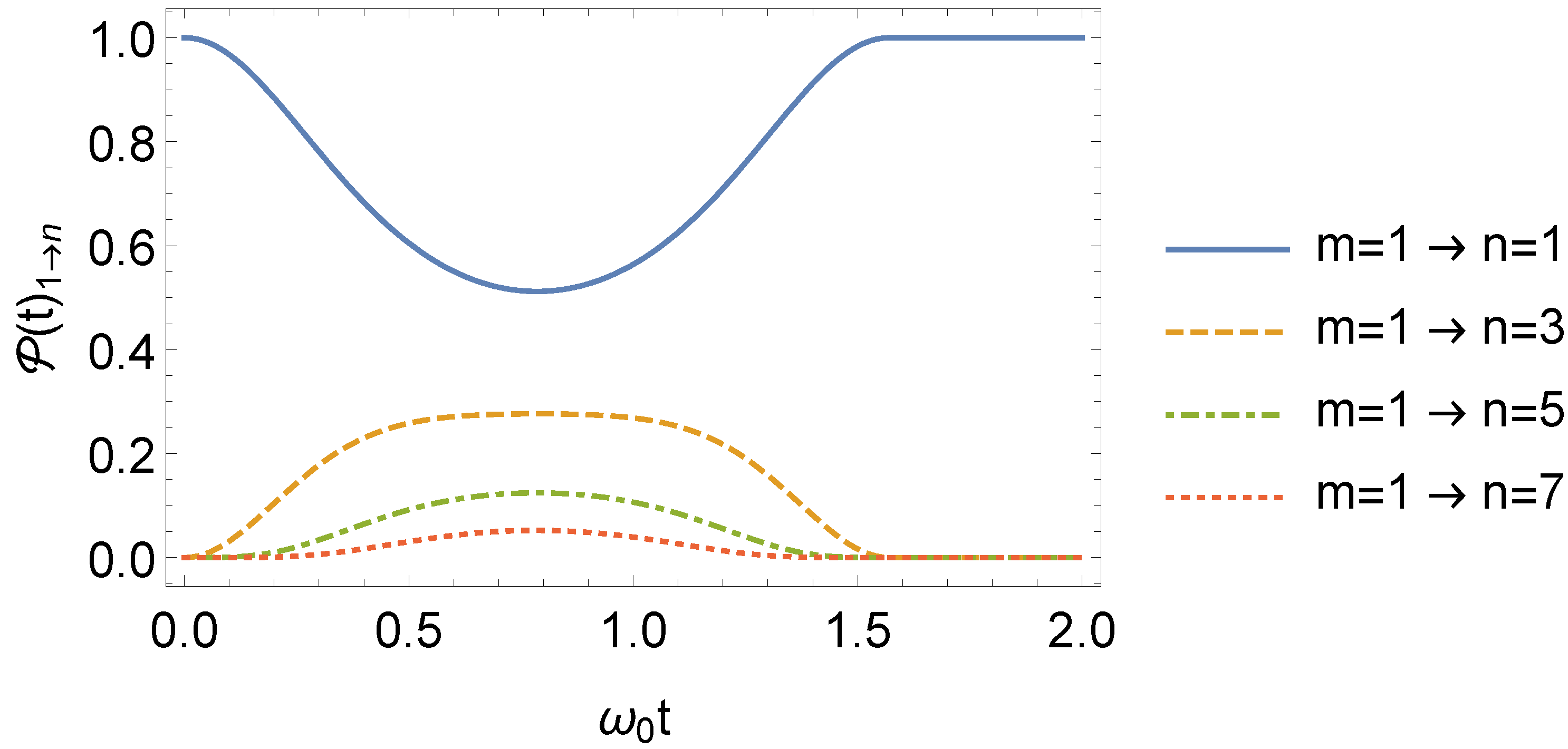
3.6. Transition Probability

The general transition probability, $\mathcal{P}{\left(t\right)}_{m\to n}$, for the model in Equation (30), is given by

$$\begin{array}{c}\hfill \mathcal{P}{\left(t\right)}_{m\to n}=\left\{\begin{array}{cc}{\delta }_{m,n},\hfill & t<0,\hfill \\ {\mathcal{P}}_1{\left(t\right)}_{m\to n},\hfill & 0<t<\tau ,\hfill \\ {\mathcal{P}}_2{\left(t\right)}_{m\to n},\hfill & t>\tau ,\hfill \end{array}\right.\end{array}$$

(66)

with ${\delta }_{m,n}$ being the Kronecker delta. Using Equations (28) and (45) (or Equations (29) and (63) with $n=0$), we find, for the interval $0<t<\tau$, ${\mathcal{P}}_1{\left(t\right)}_{m\to n}$, whose expression is

$$\begin{array}{c}\hfill {\mathcal{P}}_1{\left(t\right)}_{m\to n}=\frac{2^{m+n}min(m,n){!}^2{\left[\left(\frac{{\omega }_1^2-{\omega }_0^2}{2{\omega }_0{\omega }_1}\right)sin\left({\omega }_{1}t\right)\right]}^{|n-m|}}{m!n!{\left[1+{\left(\frac{{\omega }_1^2-{\omega }_0^2}{2{\omega }_0{\omega }_1}\right)}^2{sin}^2\left({\omega }_{1}t\right)\right]}^{\frac{1}{2}}}\\ \hfill \times {\left[\sum _{k=\frac{|n-m|}{2}}^{\frac{n+m}{2}}\frac{\left(\begin{array}{c}\frac{n+m}{2}\\ k\end{array}\right)\left(\begin{array}{c}\frac{n+m+2k-2}{4}\\ \frac{n+m}{2}\end{array}\right)k!}{\left(k-\frac{|n-m|}{2}\right)!{\left[1+{\left(\frac{{\omega }_1^2-{\omega }_0^2}{2{\omega }_0{\omega }_1}\right)}^2{sin}^2\left({\omega }_{1}t\right)\right]}^{\frac{k}{2}}}\right]}^2,\end{array}$$

(67)

for even values of $|n-m|$, and $\mathcal{P}{\left(t\right)}_{m\to n}=0$ for odd values of $|n-m|$. Since the $r_1\left(t\right)$ parameter (Equation (45)) in this interval is explicitly time-dependent, consequently, the transition probability $m\to n$ will also depend.

For the interval $t>\tau$, using Equation (46) in Equation (28) (or Equations (29) and (64) with $n=0$), we see that the result is

$$\begin{array}{c}\hfill {\mathcal{P}}_2{\left(t\right)}_{m\to n}={\mathcal{P}}_1{\left(\tau \right)}_{m\to n}.\end{array}$$

(68)

Thus, even when the frequency returns to ${\omega }_0$ after an instant $\tau$, one can find a nonzero $m\to n$ transition probability, depending on the value of $\tau$. It is noticeable from Equation (67) that $\mathcal{P}{\left(t\right)}_{m\to n}=\mathcal{P}{\left(t\right)}_{n\to m}$, with such symmetry being a consequence of the parity of the potential in Equation (7) [61]. The behavior of $\mathcal{P}{\left(t\right)}_{1\to n}$ is illustrated in Figure 11 (for $\tau =3{\tau }_1/2$) and Figure 12 (for $\tau ={\tau }_1$). In Figure 11, as n increases, $\mathcal{P}{\left(t\right)}_{1\to n}$ decreases. We highlight that for $t>\tau ={\tau }_1$ in Figure 12, $\mathcal{P}{\left(t\right)}_{1\to 1}=1$ or, in other words, the oscillator remains in its same initial state.

In addition, for $m=0$, Equation (68) gives

$$\begin{array}{c}\hfill {\mathcal{P}}_2{\left(t\right)}_{0\to n}=\frac{n!{\left(\frac{{\omega }_1^2-{\omega }_0^2}{2{\omega }_0{\omega }_1}\right)}^n{sin}^n\left({\omega }_1\tau \right)}{2^n{\left(\frac{n}{2}!\right)}^2{\left[1+{\left(\frac{{\omega }_1^2-{\omega }_0^2}{2{\omega }_0{\omega }_1}\right)}^2{sin}^2\left({\omega }_1\tau \right)\right]}^{\frac{n+1}{2}}},\end{array}$$

(69)

where $n=0,2,4,\dots ,$ recovering one of the results found in ref. [40]. Thus, Equation (68) generalizes the result for the transition probability found in ref. [40]. By also making $n=0$ in Equation (69), we find the probability of the oscillator of persisting in the fundamental state, and the probability of the oscillator being excited, after the frequency returns to ${\omega }_0$, which is given by $1-{\mathcal{P}}_2{\left(t\right)}_{0\to 0}$.

4. Final Remarks

Using the Lewis–Riesenfeld method, we investigated the dynamics of a quantum harmonic oscillator that undergoes two abrupt jumps in its frequency (Equation (30)). We reobtained the analytical formulas of ref. [40] for the squeeze parameters (Equations (45), (46), and (48)), the quantum fluctuations of the position (Equation (51)) and momentum (Equation (54)) operators, and the probability amplitude of a transition from the fundamental state to an arbitrary energy eigenstate (Equation (69)). We also obtained expressions for the mean energy value (Equations (58) and (59)), the mean number of excitations (Equations (63) and (64)) (which were not calculated in ref. [40]), and for the transition probabilities considering the initial state different from the fundamental (Equations (67) and (68)) (which generalizes the formula found in ref. [40]).

We found that, as expected, the mean energy of the system is independent of time in each one of the intervals: $t<0$, $0<t<\tau$, and $t>\tau$. Moreover, we showed that the mean energy of the oscillator after the jumps is equal or greater than that before these jumps, even when ${\omega }_1<{\omega }_0$. We also obtained, for $t>\tau \ne {\tau }_l$, a non-null value for the mean number of excitations when the oscillator starts in the fundamental state (Equations (58) and (59) with $n=0$), which means that, under the jumps in its frequency, a quantum oscillator, initially in the ground state, can become excited. We showed that transitions between arbitrary m and n states only occur if $|n-m|$ is an even number. We highlighted that, for $t>\tau \ne {\tau }_l$ and a fixed value of m, as n increases, $\mathcal{P}{\left(t\right)}_{m\to n}$ decreases. Finally, we showed that, for $t>\tau ={\tau }_l$, $\mathcal{P}{\left(t\right)}_{m\to n}={\delta }_{m,n}$, so that the oscillator returns to the same initial state (this generalizes, for any initial state m, the result found in ref. [40] for $m=0$).

References

1. Husimi, K. Miscellanea in Elementary Quantum Mechanics, II. Prog. Theor. Phys. 1953, 9, 381–402. [Google Scholar] [CrossRef]
2. Lewis, H.R. Classical and Quantum Systems with Time-Dependent Harmonic-Oscillator-Type Hamiltonians. Phys. Rev. Lett. 1967, 18, 510–512. [Google Scholar] [CrossRef]
3. Lewis, H.R. Class of Exact Invariants for Classical and Quantum Time-Dependent Harmonic Oscillators. J. Math. Phys. 1968, 9, 1976–1986. [Google Scholar] [CrossRef]
4. Lewis, H.R.; Riesenfeld, W.B. An Exact Quantum Theory of the Time-Dependent Harmonic Oscillator and of a Charged Particle in a Time-Dependent Electromagnetic Field. J. Math. Phys. 1969, 10, 1458–1473. [Google Scholar] [CrossRef]
5. Pedrosa, I.A. Exact wave functions of a harmonic oscillator with time-dependent mass and frequency. Phys. Rev. A 1997, 55, 3219–3221. [Google Scholar] [CrossRef]
6. Ciftja, O. A simple derivation of the exact wavefunction of a harmonic oscillator with time-dependent mass and frequency. J. Phys. A. Math. Gen. 1999, 32, 6385–6389. [Google Scholar] [CrossRef]
7. Guasti, M.F.; Moya-Cessa, H. Solution of the Schrödinger equation for time-dependent 1D harmonic oscillators using the orthogonal functions invariant. J. Phys. A. Math. Gen. 2003, 36, 2069–2076. [Google Scholar] [CrossRef]
8. Pedrosa, I.A.; Rosas, A. Electromagnetic Field Quantization in Time-Dependent Linear Media. Phys. Rev. Lett. 2009, 103, 010402. [Google Scholar] [CrossRef]
9. Pedrosa, I.A. Quantum electromagnetic waves in nonstationary linear media. Phys. Rev. A 2011, 83, 032108. [Google Scholar] [CrossRef]
10. Dodonov, V.; Man’ko, V.; Polynkin, P. Geometrical squeezed states of a charged particle in a time-dependent magnetic field. Phys. Lett. A 1994, 188, 232–238. [Google Scholar] [CrossRef]
11. Xu, X.-W.; Ren, T.-Q.; Liu, S.-D. Analytic solution for one-dimensional quantum oscillator with a variable frequency. Acta Phys. Sin. 1999, 8, 641–645. [Google Scholar] [CrossRef]
12. Aguiar, V.; Guedes, I. Entropy and information of a spinless charged particle in time-varying magnetic fields. J. Math. Phys. 2016, 57, 092103. [Google Scholar] [CrossRef]
13. Dodonov, V.V.; Horovits, M.B. Squeezing of Relative and Center-of-Orbit Coordinates of a Charged Particle by Step-Wise Variations of a Uniform Magnetic Field with an Arbitrary Linear Vector Potential. J. Russ. Laser Res. 2018, 39, 389–400. [Google Scholar] [CrossRef]
14. Brown, L.S. Quantum motion in a Paul trap. Phys. Rev. Lett. 1991, 66, 527–529. [Google Scholar] [CrossRef]
15. Agarwal, G.S.; Kumar, S.A. Exact quantum-statistical dynamics of an oscillator with time-dependent frequency and generation of nonclassical states. Phys. Rev. Lett. 1991, 67, 3665–3668. [Google Scholar] [CrossRef]
16. Mihalcea, B.M. A quantum parametric oscillator in a radiofrequency trap. Phys. Scr. 2009, T135, 014006. [Google Scholar] [CrossRef] [Green Version]
17. Aguiar, V.; Nascimento, J.; Guedes, I. Exact wave functions and uncertainties for a spinless charged particle in a time-dependent Penning trap. Int. J. Mass Spectrom. 2016, 409, 21–28. [Google Scholar] [CrossRef]
18. Menicucci, N.C.; Milburn, G.J. Single trapped ion as a time-dependent harmonic oscillator. Phys. Rev. A 2007, 76, 052105. [Google Scholar] [CrossRef] [Green Version]
19. Pedrosa, I.A. On the Quantization of the London Superconductor. Braz. J. Phys. 2021, 51, 401–405. [Google Scholar] [CrossRef]
20. Choi, J.R. Interpreting quantum states of electromagnetic field in time-dependent linear media. Phys. Rev. A 2010, 82, 055803. [Google Scholar] [CrossRef]
21. Salamon, P.; Hoffmann, K.H.; Rezek, Y.; Kosloff, R. Maximum work in minimum time from a conservative quantum system. Phys. Chem. Chem. Phys. 2009, 11, 1027–1032. [Google Scholar] [CrossRef] [PubMed]
22. Schaff, J.F.; Song, X.L.; Vignolo, P.; Labeyrie, G. Fast optimal transition between two equilibrium states. Phys. Rev. A 2010, 82, 033430. [Google Scholar] [CrossRef] [Green Version]
23. Chen, X.; Ruschhaupt, A.; Schmidt, S.; del Campo, A.; Guéry-Odelin, D.; Muga, J.G. Fast Optimal Frictionless Atom Cooling in Harmonic Traps: Shortcut to Adiabaticity. Phys. Rev. Lett. 2010, 104, 063002. [Google Scholar] [CrossRef]
24. Stefanatos, D.; Ruths, J.; Li, J.S. Frictionless atom cooling in harmonic traps: A time-optimal approach. Phys. Rev. A 2010, 82, 063422. [Google Scholar] [CrossRef] [Green Version]
25. Dupays, L.; Spierings, D.C.; Steinberg, A.M.; del Campo, A. Delta-kick cooling, time-optimal control of scale-invariant dynamics, and shortcuts to adiabaticity assisted by kicks. Phys. Rev. Res. 2021, 3, 033261. [Google Scholar] [CrossRef]
26. Martínez-Tibaduiza, D.; Pires, L.; Farina, C. Time-dependent quantum harmonic oscillator: A continuous route from adiabatic to sudden changes. J. Phys. B At. Mol. Opt. Phys. 2021, 54, 205401. [Google Scholar] [CrossRef]
27. Landim, R.R.; Guedes, I. Wave functions for a Dirac particle in a time-dependent potential. Phys. Rev. A 2000, 61, 054101. [Google Scholar] [CrossRef]
28. Gao, X.C.; Fu, J.; Li, X.H.; Gao, J. Invariant formulation and exact solutions for the relativistic charged Klein-Gordon field in a time-dependent spatially homogeneous electric field. Phys. Rev. A 1998, 57, 753–761. [Google Scholar] [CrossRef]
29. Dodonov, V.V.; Klimov, A.B. Generation and detection of photons in a cavity with a resonantly oscillating boundary. Phys. Rev. A 1996, 53, 2664–2682. [Google Scholar] [CrossRef]
30. Dodonov, V.; Klimov, A.; Man’ko, V. Generation of squeezed states in a resonator with a moving wall. Phys. Lett. A 1990, 149, 225–228. [Google Scholar] [CrossRef]
31. Pedrosa, I.A.; Guedes, I. Exact quantum states of an inverted pendulum under time-dependent gravitation. Int. J. Mod. Phys. A 2004, 19, 4165–4172. [Google Scholar] [CrossRef]
32. Carvalho, A.M.d.M.; Furtado, C.; Pedrosa, I.A. Scalar fields and exact invariants in a Friedmann-Robertson-Walker spacetime. Phys. Rev. D 2004, 70, 123523. [Google Scholar] [CrossRef]
33. Greenwood, E. Time-dependent particle production and particle number in cosmological de Sitter space. Int. J. Mod. Phys. D 2015, 24, 1550031. [Google Scholar] [CrossRef] [Green Version]
34. Janszky, J.; Yushin, Y. Squeezing via frequency jump. Opt. Commun. 1986, 59, 151–154. [Google Scholar] [CrossRef]
35. Janszky, J.; Adam, P. Strong squeezing by repeated frequency jumps. Phys. Rev. A 1992, 46, 6091–6092. [Google Scholar] [CrossRef] [PubMed]
36. Kiss, T.; Janszky, J.; Adam, P. Time evolution of harmonic oscillators with time-dependent parameters: A step-function approximation. Phys. Rev. A 1994, 49, 4935–4942. [Google Scholar] [CrossRef] [PubMed]
37. Moya-Cessa, H.; Fernández Guasti, M. Coherent states for the time dependent harmonic oscillator: The step function. Phys. Lett. A 2003, 311, 1–5. [Google Scholar] [CrossRef] [Green Version]
38. Stefanatos, D. Minimum-Time Transitions between Thermal and Fixed Average Energy States of the Quantum Parametric Oscillator. SIAM J. Control Optim. 2017, 55, 1429–1451. [Google Scholar] [CrossRef] [Green Version]
39. Stefanatos, D. Minimum-Time Transitions Between Thermal Equilibrium States of the Quantum Parametric Oscillator. IEEE Trans. Automat. Contr. 2017, 62, 4290–4297. [Google Scholar] [CrossRef] [Green Version]
40. Tibaduiza, D.M.; Pires, L.; Szilard, D.; Zarro, C.A.D.; Farina, C.; Rego, A.L.C. A Time-Dependent Harmonic Oscillator with Two Frequency Jumps: An Exact Algebraic Solution. Braz. J. Phys. 2020, 50, 634–646. [Google Scholar] [CrossRef]
41. Tibaduiza, D.M.; Pires, L.; Rego, A.L.C.; Szilard, D.; Zarro, C.; Farina, C. Efficient algebraic solution for a time-dependent quantum harmonic oscillator. Phys. Scr. 2020, 95, 105102. [Google Scholar] [CrossRef]
42. Pedrosa, I.A.; Serra, G.P.; Guedes, I. Wave functions of a time-dependent harmonic oscillator with and without a singular perturbation. Phys. Rev. A 1997, 56, 4300–4303. [Google Scholar] [CrossRef]
43. Xin, M.; Leong, W.S.; Chen, Z.; Wang, Y.; Lan, S.Y. Rapid Quantum Squeezing by Jumping the Harmonic Oscillator Frequency. Phys. Rev. Lett. 2021, 127, 183602. [Google Scholar] [CrossRef] [PubMed]
44. Wolf, F.; Shi, C.; Heip, J.C.; Gessner, M.; Pezzè, L.; Smerzi, A.; Schulte, M.; Hammerer, K.; Schmidt, P.O. Motional Fock states for quantum-enhanced amplitude and phase measurements with trapped ions. Nat. Commun. 2019, 10, 2929. [Google Scholar] [CrossRef] [Green Version]
45. Choi, J.R. The dependency on the squeezing parameter for the uncertainty relation in the squeezed states of the time-dependent oscillator. Int. J. Mod. Phys. B 2004, 18, 2307–2324. [Google Scholar] [CrossRef]
46. Sakurai, J.J.; Napolitano, J. Modern Quantum Mechanics, 3rd ed.; Cambridge University Press: Cambridge, UK, 2020; pp. 83–88. [Google Scholar]
47. Griffiths, D.J. Introduction to Quantum Mechanics, 3rd ed.; Cambridge University Press: Cambridge, UK, 2018; pp. 39–55. [Google Scholar]
48. Cohen-Tannoudji, C.; Diu, B.; Laloe, F. Quantum Mechanics, Volume 1: Basic Concepts, Tools, and Applications, 2nd ed.; Wiley-VCH: Weinheim, Germany, 2019; pp. 502–521. [Google Scholar]
49. Prykarpatskyy, Y. Steen–Ermakov–Pinney Equation and Integrable Nonlinear Deformation of the One-Dimensional Dirac Equation. J. Math. Sci. 2018, 231, 820–826. [Google Scholar] [CrossRef] [Green Version]
50. Pinney, E. The nonlinear differential equation y″ + p(x)y + cy−3 = 0. Proc. Am. Math. Soc. 1950, 1, 681. [Google Scholar] [CrossRef]
51. de Lima, A.L.; Rosas, A.; Pedrosa, I. Quantum dynamics of a particle trapped by oscillating fields. J. Mod. Opt. 2009, 56, 75–80. [Google Scholar] [CrossRef]
52. Cariñena, J.F.; de Lucas, J. Applications of Lie systems in dissipative Milne-Pinney equations. Int. J. Geom. Methods Mod. Phys. 2009, 06, 683–699. [Google Scholar] [CrossRef] [Green Version]
53. Weber, H.J.; Arfken, G.B. Essential Mathematical Methods for Physicists, 6th ed.; Academic Press: San Diego, CA, USA, 2003; pp. 638–642. [Google Scholar]
54. Pedrosa, I.A. Comment on “Coherent states for the time-dependent harmonic oscillator”. Phys. Rev. D 1987, 36, 1279–1280. [Google Scholar] [CrossRef]
55. Daneshmand, R.; Tavassoly, M.K. Dynamics of Nonclassicality of Time- and Conductivity-Dependent Squeezed States and Excited Even/Odd Coherent States. Commun. Theor. Phys. 2017, 67, 365–376. [Google Scholar] [CrossRef]
56. Guerry, C.C.; Knight, P.L. Introductory Quantum Optics, 1st ed.; Cambridge University Press: Cambridge, UK, 2005; pp. 150–165. [Google Scholar]
57. Kim, M.S.; de Oliveira, F.A.M.; Knight, P.L. Properties of squeezed number states and squeezed thermal states. Phys. Rev. A 1989, 40, 2494–2503. [Google Scholar] [CrossRef] [PubMed]
58. Marian, P. Higher-order squeezing and photon statistics for squeezed thermal states. Phys. Rev. A 1992, 45, 2044–2051. [Google Scholar] [CrossRef]
59. Moeckel, M.; Kehrein, S. Real-time evolution for weak interaction quenches in quantum systems. Ann. Phys. (N. Y). 2009, 324, 2146–2178. [Google Scholar] [CrossRef] [Green Version]
60. Kim, M.; de Oliveira, F.; Knight, P. Photon number distributions for squeezed number states and squeezed thermal states. Opt. Commun. 1989, 72, 99–103. [Google Scholar] [CrossRef]
61. Popov, V.; Perelomov, A. Parametric Excitation of a Quantum Oscillator. Sov. J. Exp. Theor. Phys. 1969, 30, 1375–1390. [Google Scholar]
Figure 1. General behavior of ρ ( t ) , as a function of ω 0 t , with ω 1 = 3 ω 0 and different values of τ (we consider, for simplicity, m 0 = ω 0 = 1 and = 1 in arbitrary units). For τ = [ τ l + 1 / 2 ] l = 2 = 5 π / 6 , we note that the amplitude of oscillation for the ρ ( t ) parameter is maximum. For τ = 59 π / 62 , the amplitude of oscillation is intermediate. Finally, when τ = [ τ l ] l = 3 = π , there is no oscillation at all, and it follows that ρ ( t ) becomes time independent.
Entropy 24 01851 g001
Figure 2. Behavior of the squeeze parameter r ( t ) as a function of ω 0 t , where ω 1 = 3 ω 0 (we consider ω 0 = 1 in arbitrary units).
Entropy 24 01851 g002
Figure 3. Behavior of the squeeze phase ϕ ( t ) as a function of ω 0 t , where ω 1 = 3 ω 0 (we consider ω 0 = 1 in arbitrary units).
Entropy 24 01851 g003
Figure 4. Behavior of the [ Δ x ^ ] 2 ( n , t ) for n = 0 as a function of ω 0 t , where ω 1 = 3 ω 0 (we consider, for simplicity, m 0 = ω 0 = 1 and = 1 in arbitrary units).
Entropy 24 01851 g004
Figure 5. Behavior of the [ Δ p ^ ] 2 ( n , t ) for n = 0 as a function of ω 0 t , where ω 1 = 3 ω 0 (we consider, for simplicity, m 0 = ω 0 = 1 and = 1 in arbitrary units).
Entropy 24 01851 g005
Figure 6. Behavior of the [ Δ x ^ ] 2 ( n , t ) [ Δ p ^ ] 2 ( n , t ) for n = 0 as a function of ω 0 t , where ω 1 = 3 ω 0 (we consider, for simplicity, m 0 = ω 0 = 1 and = 1 in arbitrary units).
Entropy 24 01851 g006
Figure 7. Ratio E 2 ( n , t ) / E 0 ( n ) as a function of ω 0 τ and ω 1 / ω 0 . The dashed line corresponds to ω 1 = ω 0 . The dotted lines correspond to τ = τ l . The dot–dashed lines correspond to τ = τ l + 1 / 2 .
Entropy 24 01851 g007
Figure 8. Ratio E 2 ( n , t ) / E 1 ( n , t ) as a function of ω 1 / ω 0 . For ω 1 / ω 0 < 1 , E 2 ( n , t ) / E 1 ( n , t ) > 1 , whereas for ω 1 / ω 0 > 1 , E 2 ( n , t ) / E 1 ( n , t ) 1 .
Entropy 24 01851 g008
Figure 9. Some examples of mean number of excitations N ^ 2 ( 0 , t ) that an oscillator could undergo as a function of ω 1 / ω 0 for different values of ω 0 τ .
Entropy 24 01851 g009
Figure 10. Mean number of excitations N ^ ( 0 , t ) as a function of ω 0 t for different values of τ , where ω 1 = 3 ω 0 (we consider ω 0 = 1 in arbitrary units).
Entropy 24 01851 g010
Figure 11. Behavior of P ( t ) 1 n , as a function of ω 0 t , with ω 1 = 2 ω 0 and τ = 3 τ 1 / 2 = 3 π / 4 (we consider ω 0 = 1 in arbitrary units).
Entropy 24 01851 g011
Figure 12. Behavior of P ( t ) 1 n , as a function of ω 0 t , with ω 1 = 2 ω 0 and τ = τ 1 = π / 2 (we consider ω 0 = 1 in arbitrary units).
Entropy 24 01851 g012
Publisher’s Note: MDPI stays neutral with regard to jurisdictional claims in published maps and institutional affiliations.