

Saturated Nonsingular Fast Sliding Mode Control for the Crane-Form Pipeline System


Abstract
:1. Introduction
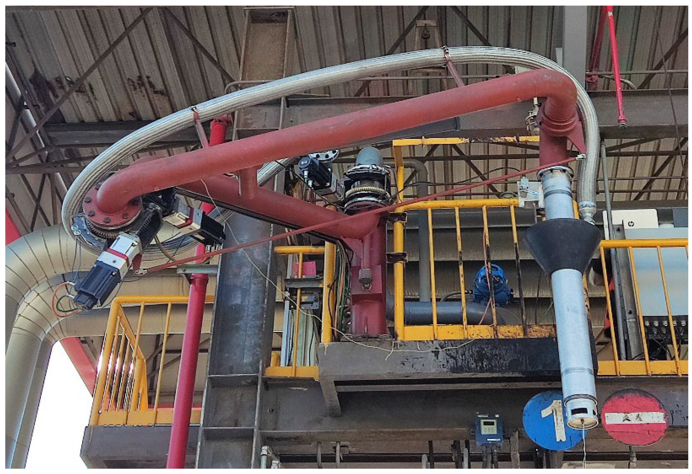
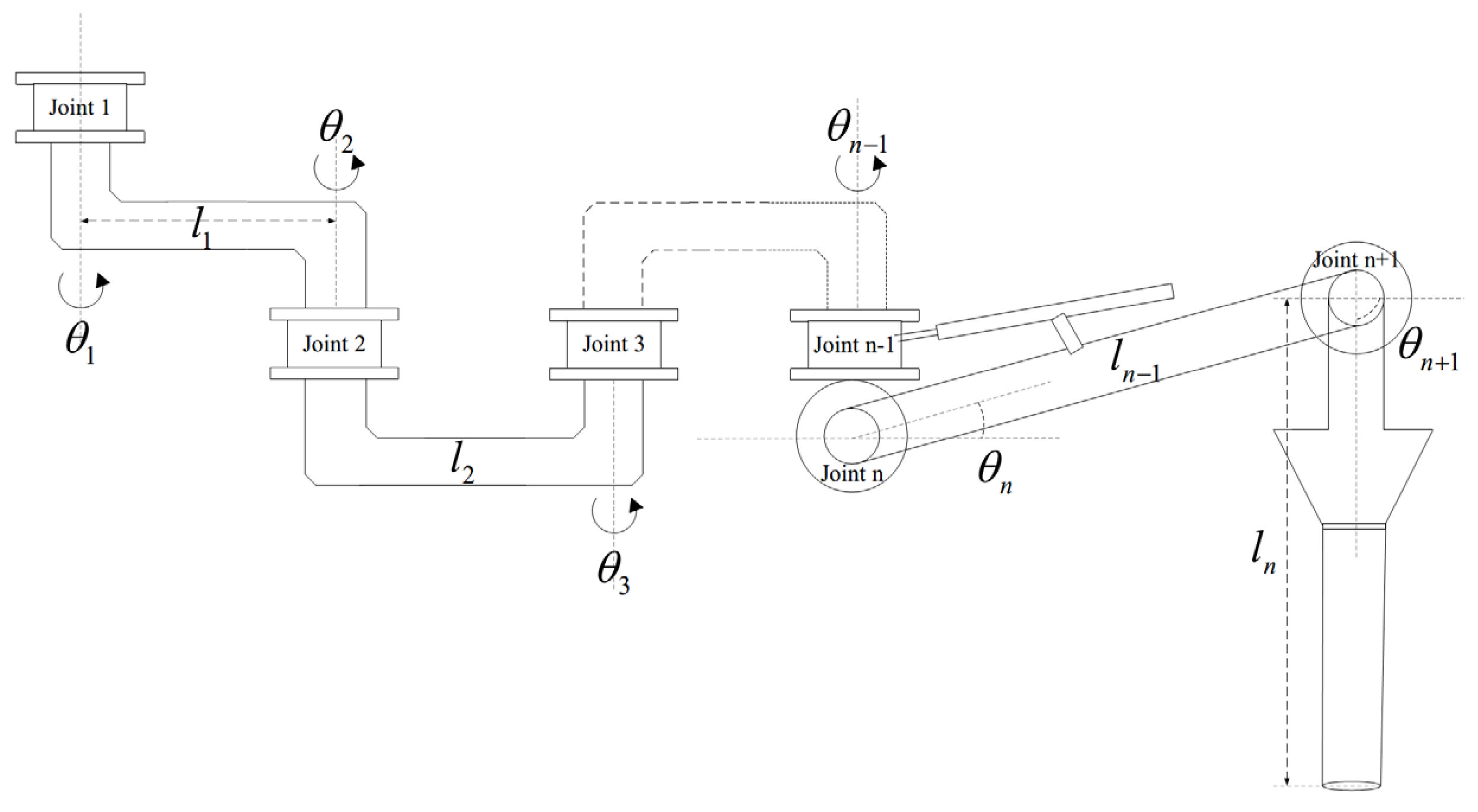
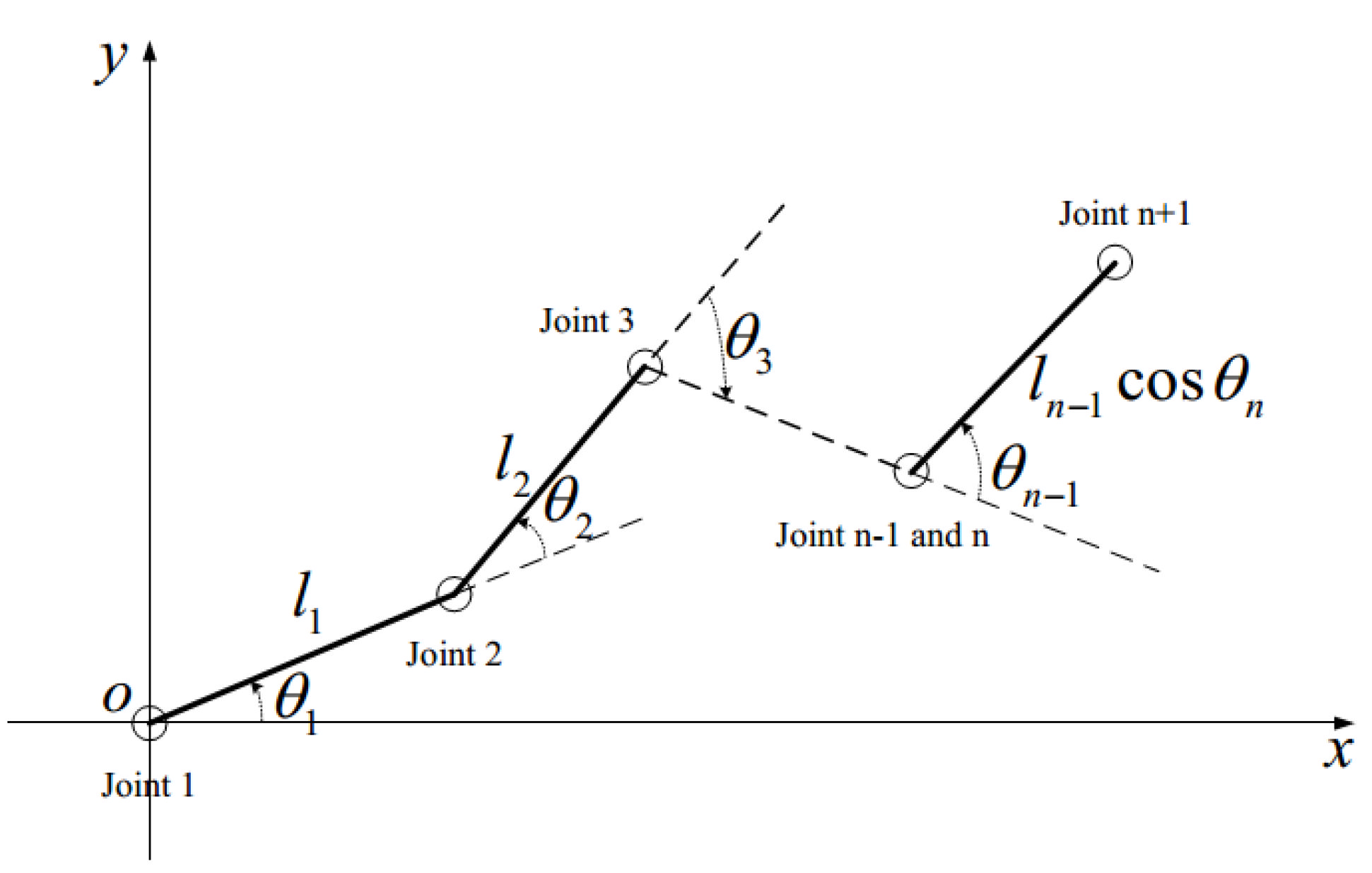
2. Dynamic Modeling
3. Control Design and Stability Analysis
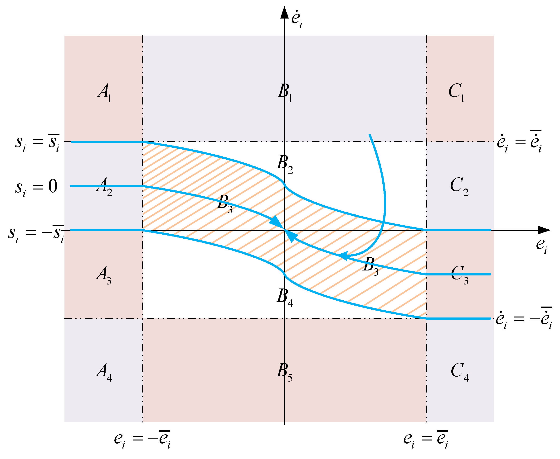
3.1. SNFTSM Algorithm
3.2. Controller Design
3.3. Stability Analysis
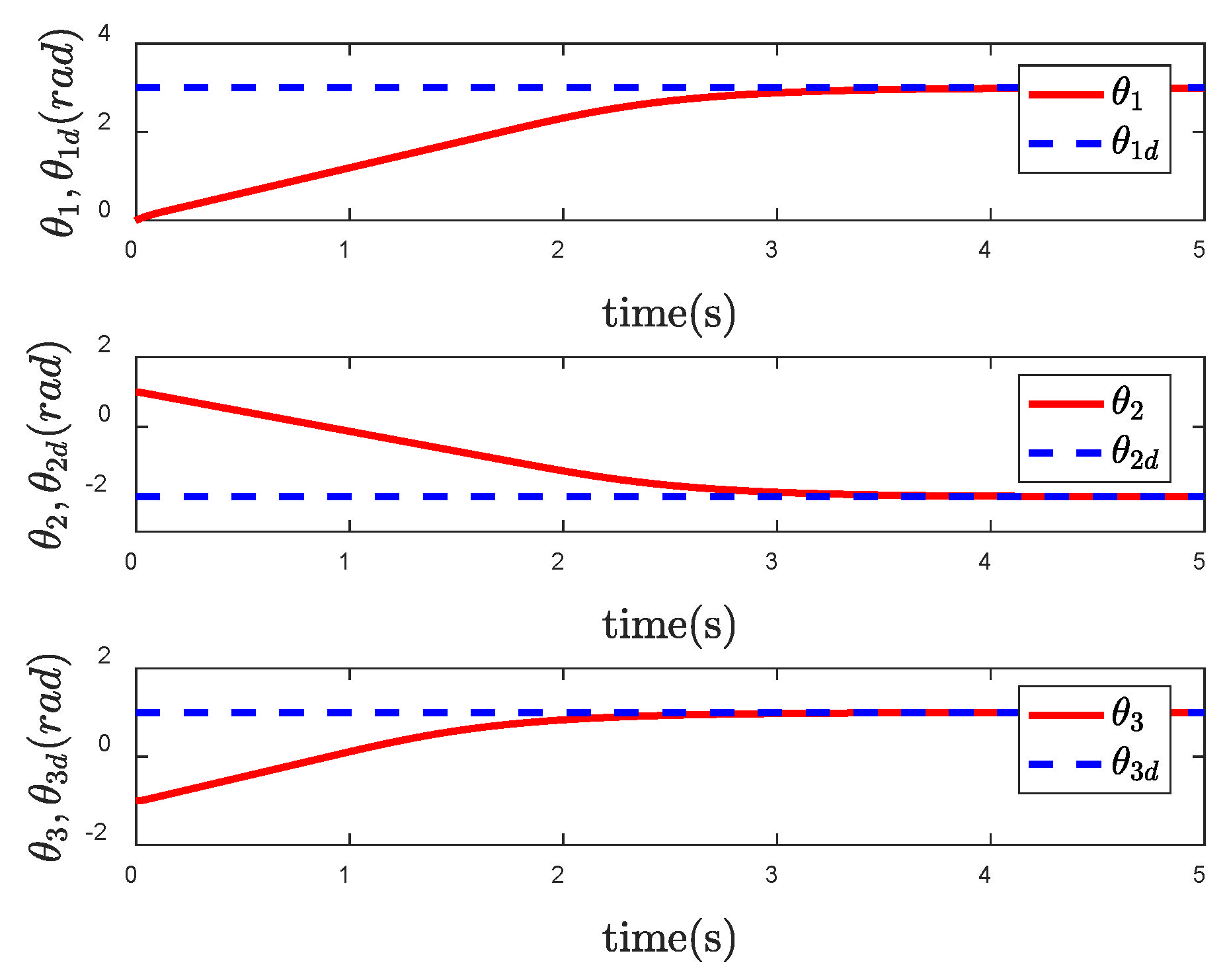
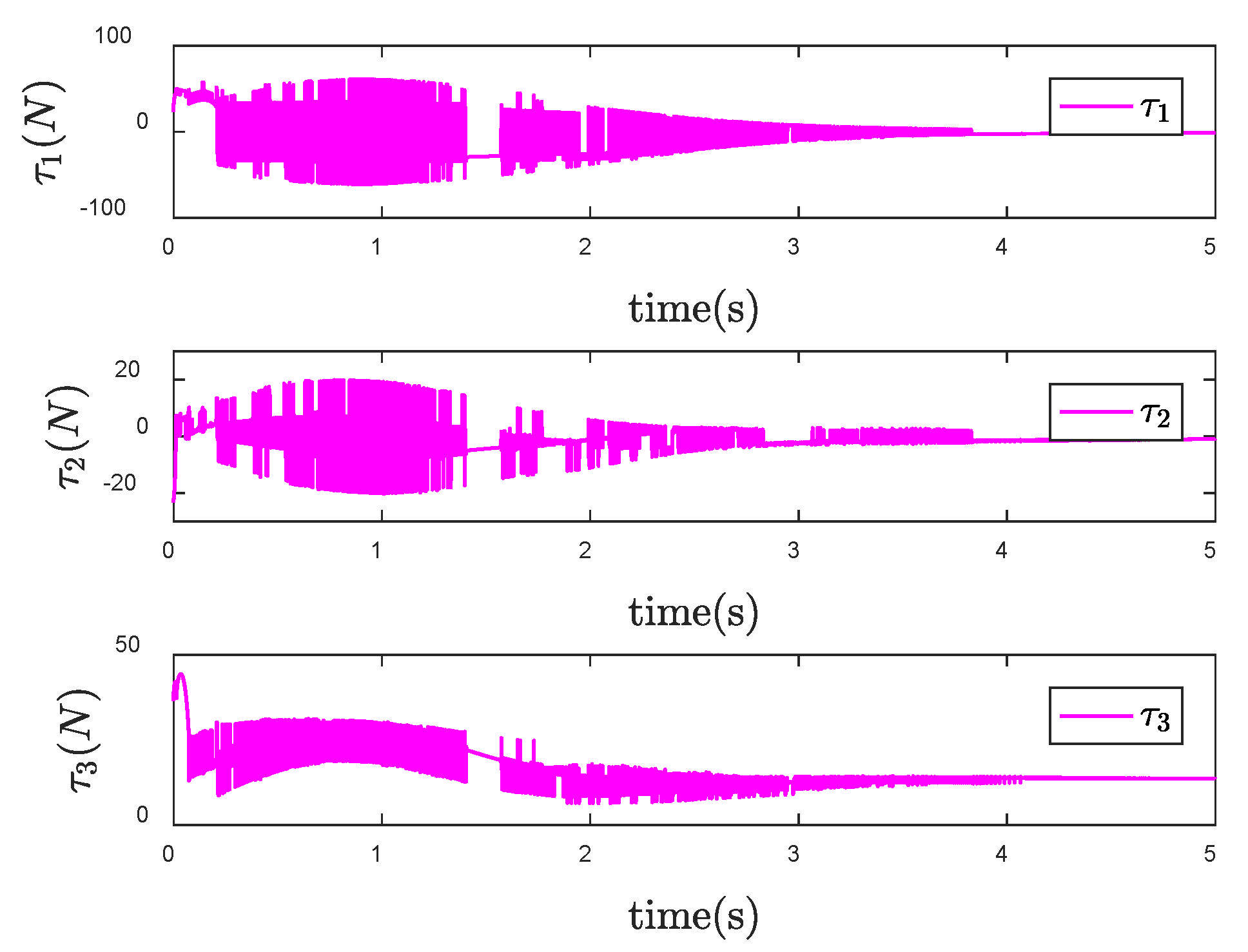
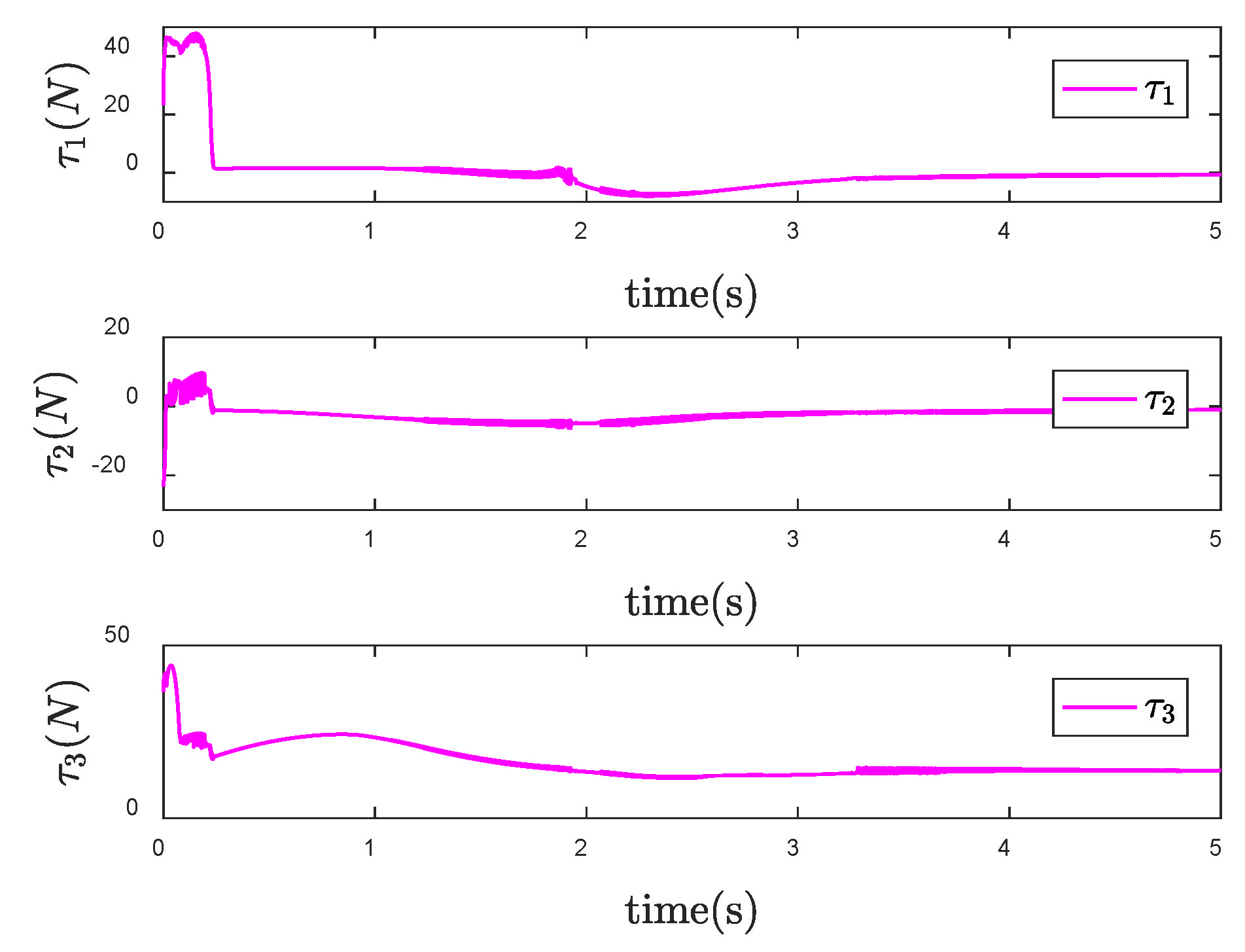
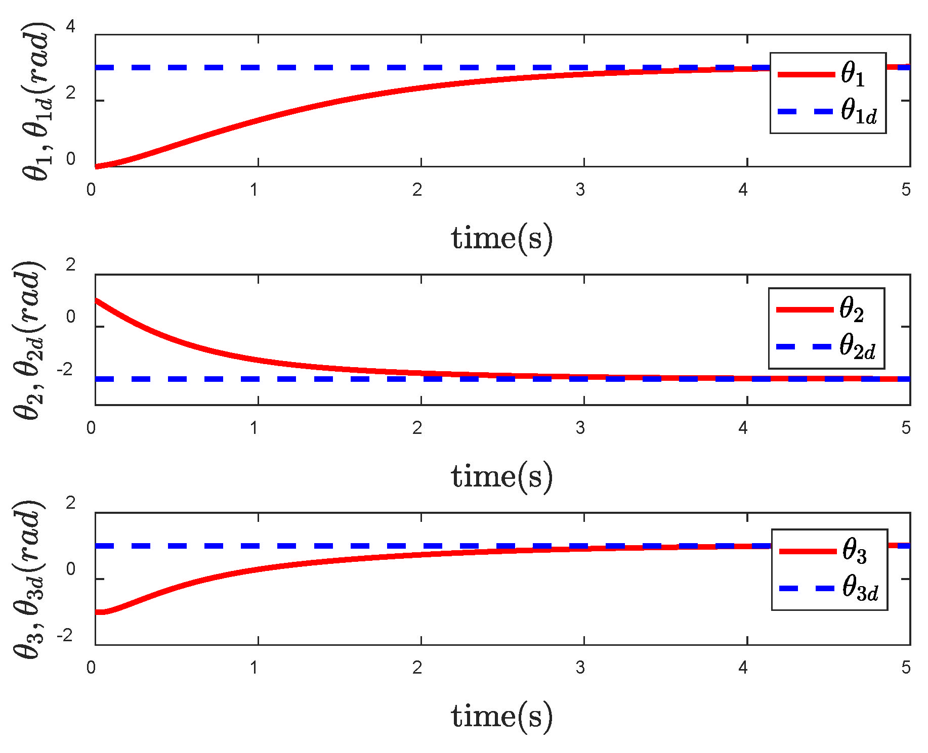
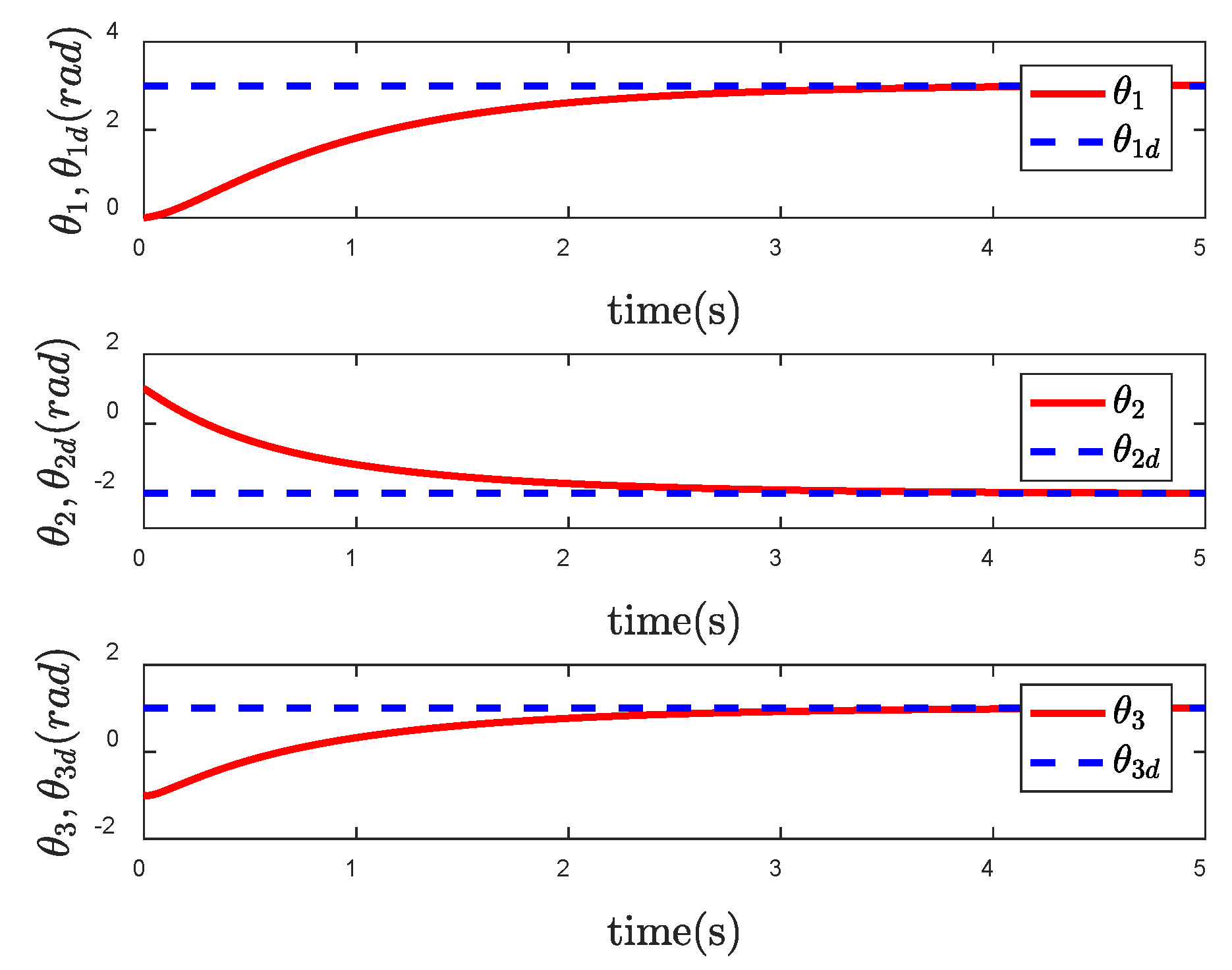
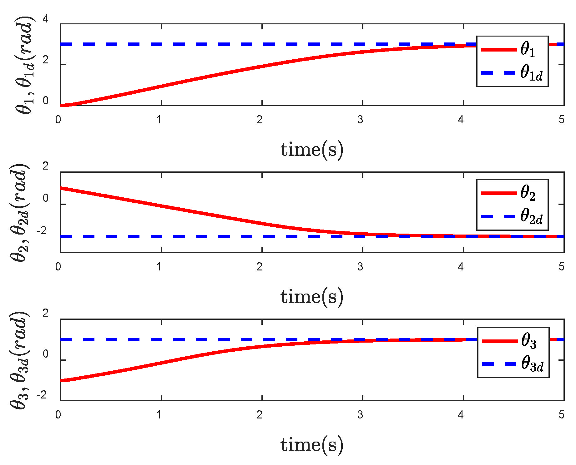
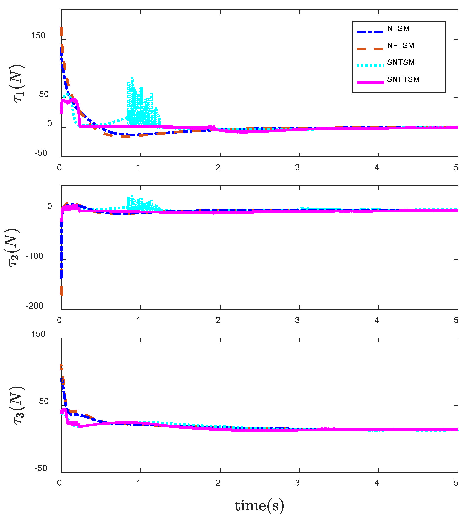
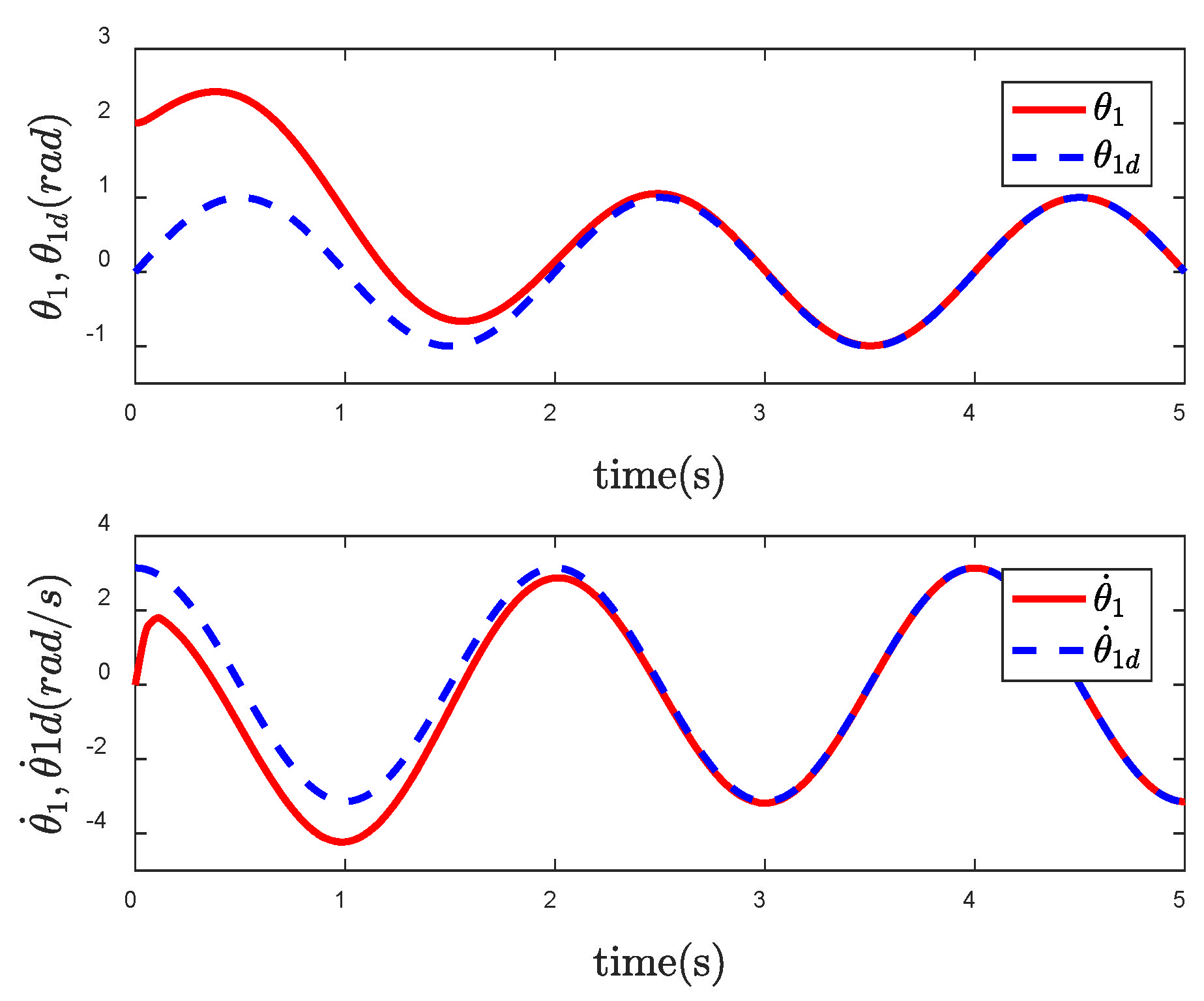
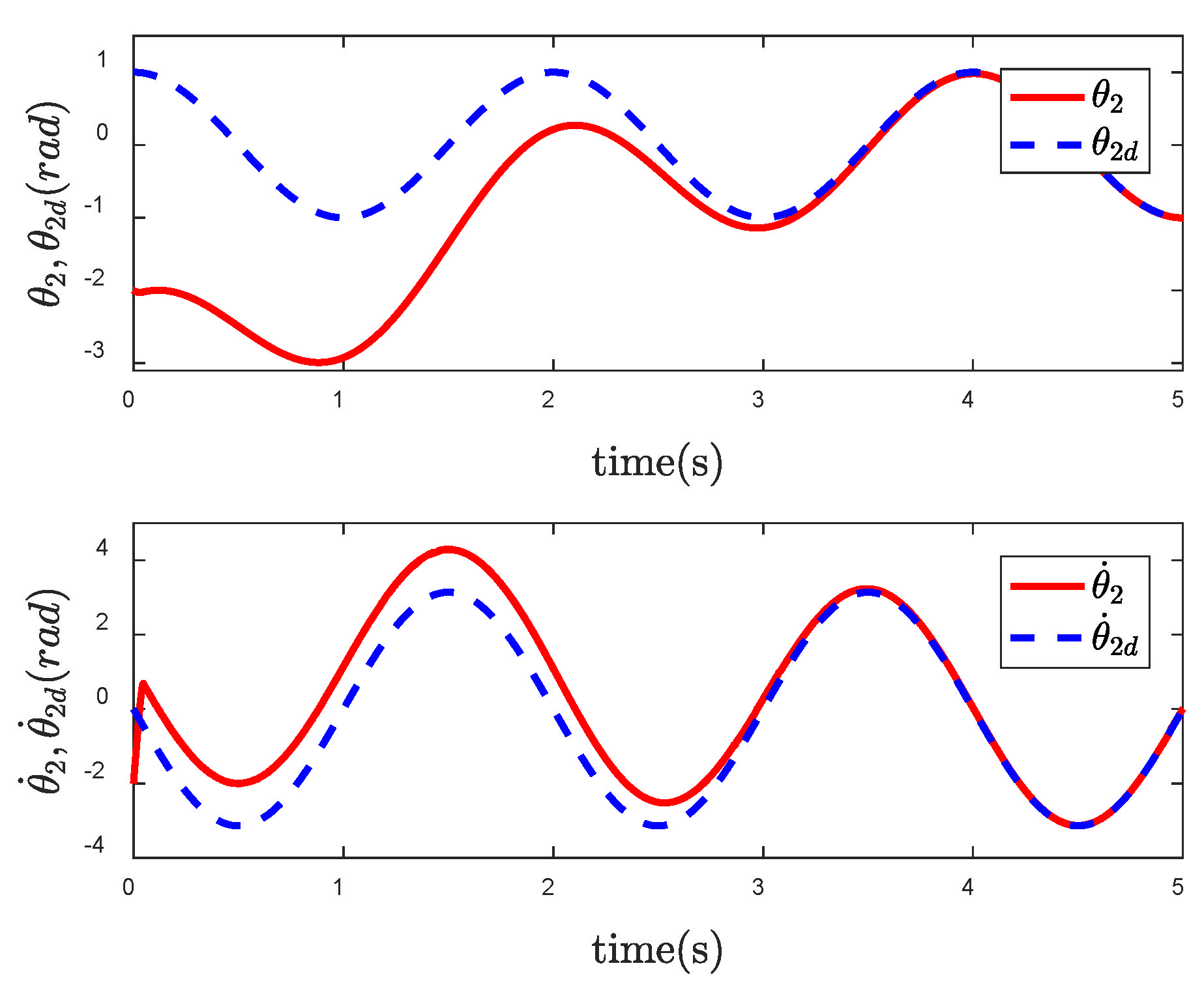
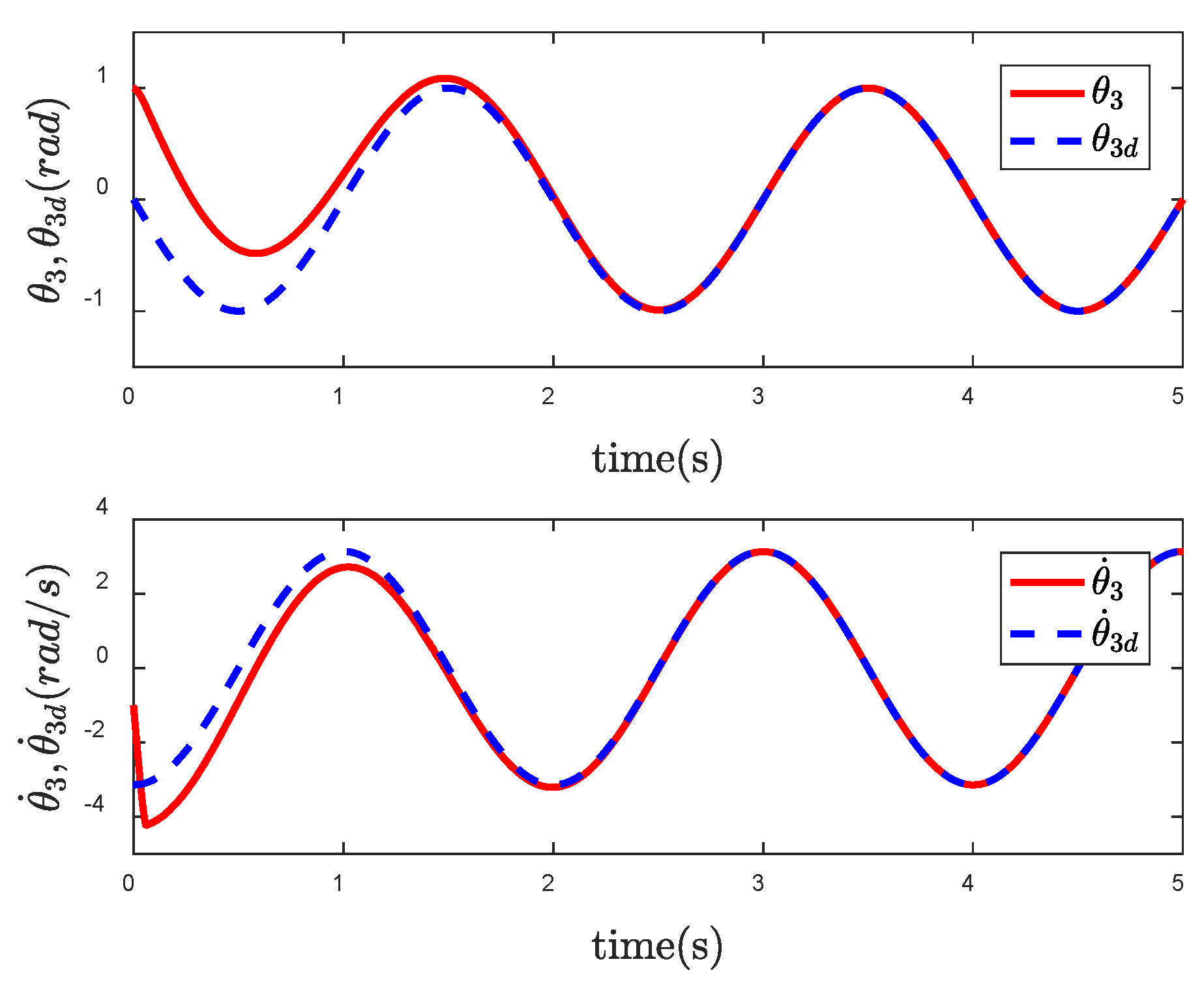
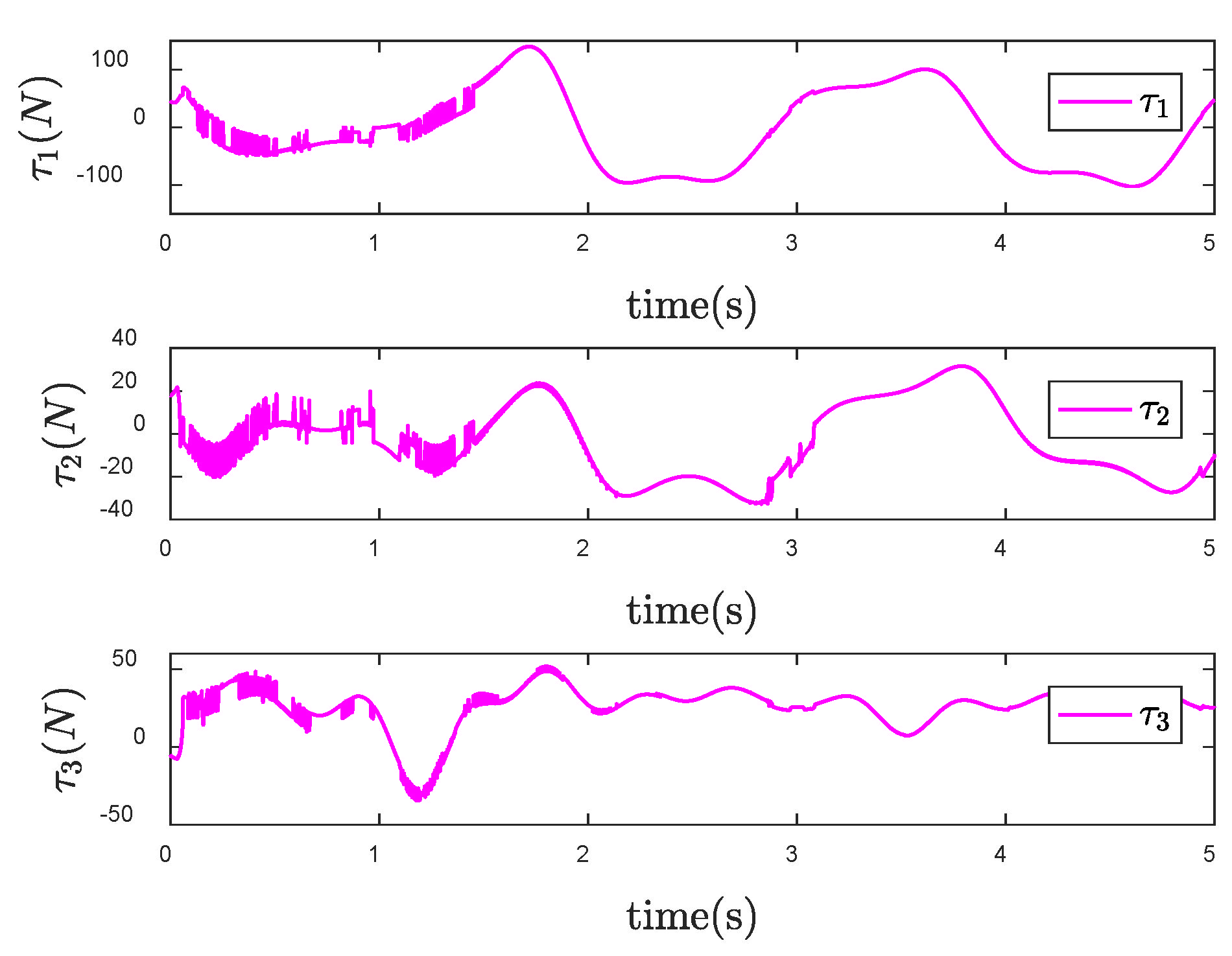
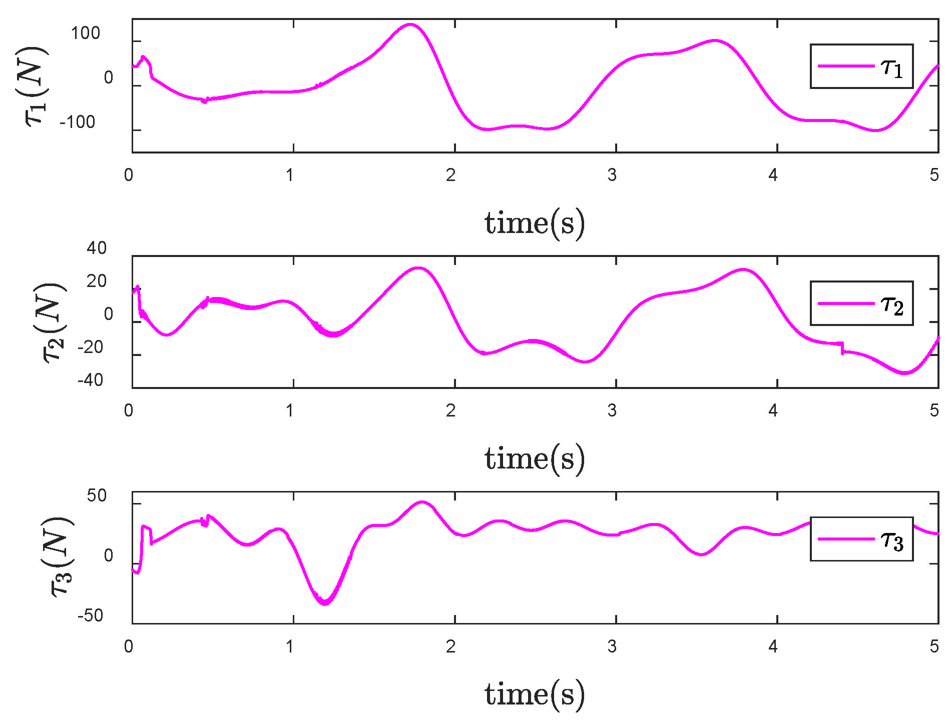
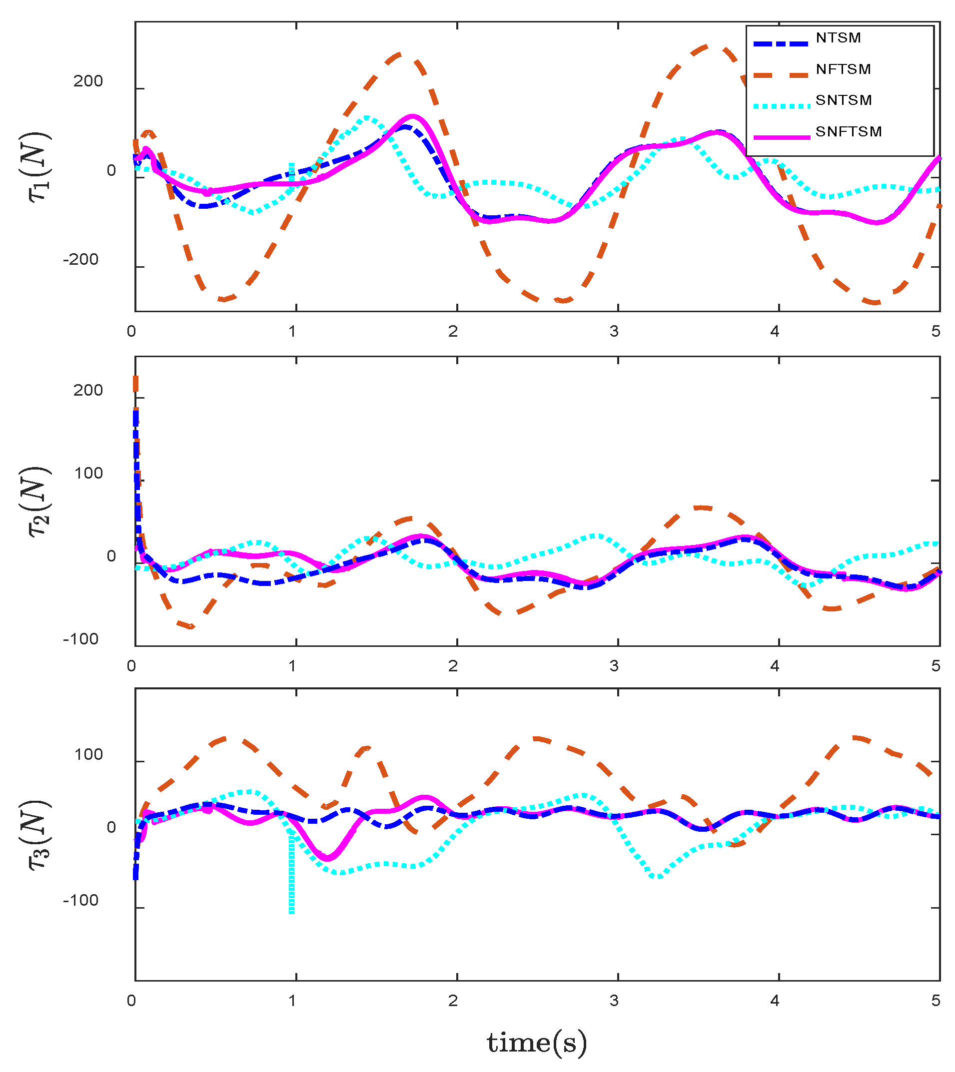
4. Simulation
5. Conclusions
Author Contributions
Funding
Institutional Review Board Statement
Informed Consent Statement
Data Availability Statement
Conflicts of Interest
References
- Park, J.; Chun, W.Y. Design of a robust H-infinity PID control for industrial manipulators. J. Dyn. Syst. Meas. Control-Trans. ASME 2000, 122, 803–812. [Google Scholar] [CrossRef]
- Anjum, Z.; Guo, Y. Finite time fractional-order adaptive backstepping fault tolerant control of robotic manipulator. Int. J. Control Autom. Syst. 2020, 19, 301–310. [Google Scholar] [CrossRef]
- Yen, V.T.; Nan, W.Y.; Cuong, P.V. Robust adaptive sliding mode neural networks control for industrial robot manipulators. Int. J. Control Autom. Syst. 2019, 17, 783–792. [Google Scholar] [CrossRef]
- Tuan, L.A.; Joo, Y.H.; Tien, L.Q.; Duong, P.X. Adaptive neural network second-order sliding mode control of dual arm robots. Int. J. Control Autom. Syst. 2017, 15, 2883–2891. [Google Scholar] [CrossRef]
- Wu, T.S.; Karkoub, M.; Wang, H.W. Robust tracking control of MIMO underactuated nonlinear systems with dead-zone band and delayed uncertainty using an adaptive fuzzy control. IEEE Trans. Fuzzy Syst. 2017, 25, 905–918. [Google Scholar] [CrossRef]
- Zhuang, H.X.; Sun, Q.L.; Chen, Z.Q.; Zeng, X. Back-stepping active disturbance rejection control for attitude control of aircraft systems based on extended state observer. Int. J. Control Autom. Syst. 2021, 19, 2134–2149. [Google Scholar] [CrossRef]
- Singh, A.M.; Ha, Q.P. Fast terminal sliding control application for second-order underactuated systems. Int. J. Control Autom. Syst. 2019, 17, 1884–1898. [Google Scholar] [CrossRef] [Green Version]
- Jafarov, E.M.; Parlakci, M.N.A.; Istefanopulos, Y. A new variable structure PID-controller design for robot manipulators. IEEE Trans. Control Syst. Technol. 2005, 13, 122–130. [Google Scholar] [CrossRef]
- Guo, Y.Z.; Woo, P.Z. An adaptive fuzzy sliding mode controller for robotic manipulators. IEEE Trans. Syst. Man Cybern. Part A: Syst. Hum. 2003, 33, 149–159. [Google Scholar] [CrossRef]
- Liu, H.T.; Zhang, T. Fuzzy sliding mode control of robotic manipulators with kinematic and dynamic uncertainties. J. Dyn. Syst. Meas. Control-Trans. ASME 2012, 134, 061007. [Google Scholar] [CrossRef]
- Shi, J.; Liu, H.; Bajcinca, N. Robust control of robotic manipulators based on integral sliding mode. Int. J. Control 2008, 81, 1537–1548. [Google Scholar] [CrossRef]
- Lee, J.; Chang, P.H.; Jin, M. Adaptive integral sliding mode control with time-delay estimation for robot manipulators. IEEE Trans. Ind. Electron. 2017, 64, 6796–6804. [Google Scholar] [CrossRef]
- Yu, S.H.; Yu, X.H.; Shirinzadeh, B.; Man, Z. Continuous finite-time control for robotic manipulators with terminal sliding mode. Automatica 2005, 41, 1957–1964. [Google Scholar] [CrossRef]
- Feng, Y.; Yu, X.H.; Man, Z.H. Non-singular terminal sliding mode control of rigid manipulators. Automatica 2002, 38, 2159–2167. [Google Scholar] [CrossRef]
- Al-Ghanimi, A.; Zhang, J.C.; Man, Z.H. Robust and fast non-singular terminal sliding mode control for piezoelectric actuators. IET Control Theory Appl. 2015, 9, 2678–2687. [Google Scholar] [CrossRef]
- Yi, S.C.; Zhai, J.Y. Adaptive second-order fast nonsingular terminal sliding mode control for robotic manipulators. ISA Trans. 2019, 90, 41–51. [Google Scholar] [CrossRef] [PubMed]
- Su, Y.X.; Zheng, C.H.; Mercorelli, P. Robust approximate fixed-time tracking control for uncertain robot manipulators. Mech. Syst. Signal Process. 2020, 135, 106379. [Google Scholar] [CrossRef]
- Yan, Y.; Wang, R.; Yu, S.H.; Wang, C.; Li, T. Event-triggered output feedback sliding mode control of mechanical systems. Nonlinear Dyn. 2022, 107, 3543–3555. [Google Scholar] [CrossRef]
- Xavier, N.; Bandyopadhyay, B. Practical sliding mode using state depended intermittent control. IEEE Trans. Circuits Syst. Ⅱ-Express Briefs 2021, 68, 341–345. [Google Scholar] [CrossRef]
- Sun, L.; Huo, W.; Jia, Z.X. Adaptive backstepping control of spacecraft rendezvous and proximity operations with input saturation and full-state constraint. IEEE Trans. Ind. Electron. 2017, 61, 480–492. [Google Scholar] [CrossRef]
- Ding, S.H.; Zheng, W.X. Nonsingular terminal sliding mode control of nonlinear second-order systems with input saturation. Int. J. Robust Nonlinear Control 2016, 26, 1857–1872. [Google Scholar] [CrossRef]
- Sun, J.G.; Sun, S.M. Tracking control of hypersonic vehicles with input saturation based on fast terminal sliding mode. Int. J. Aeronaut. Space Sci. 2019, 20, 493–505. [Google Scholar] [CrossRef]
- Guo, Y.; Huang, B.; Li, A.J.; Wang, C. Integral sliding mode control for Euler-Lagrange systems with input saturation. Int. J. Robust Nonlinear Control 2019, 29, 1088–1100. [Google Scholar] [CrossRef]
- Han, J.S.; Kim, T.I.; Oh, T.H.; Lee, S.-H.; Cho, D.-I.D. Effective disturbance compensation method under control saturation in discrete-time sliding mode control. IEEE Trans. Ind. Electron. 2020, 67, 5696–5707. [Google Scholar] [CrossRef]
- Zhang, J.J. State observer-based adaptive neural dynamic surface control for a class of uncertain nonlinear systems with input saturation using disturbance observer. Neural Comput. Appl. 2019, 31, 4993–5004. [Google Scholar] [CrossRef]
- Ma, Z.Q.; Huang, P.F. Adaptive Neural-Network Controller for an Uncertain Rigid Manipulator with Input Saturation and Full-Order State Constraint. IEEE Trans. Cybern. 2022, 52, 2907–2915. [Google Scholar] [CrossRef] [PubMed]
- Santibanez, V.; Camarillo, K.; Moreno-Valenzuela, J.; Campa, R. A practical PID regulator with bounded torques for robot manipulators. Int. J. Control Autom. Syst. 2010, 8, 544–555. [Google Scholar] [CrossRef]
- Li, Z.J.; Ge, S.Z.; Ming, A.G. Adaptive robust motion/force control of holonomic-constrained nonholonomic mobile manipulators. IEEE Trans. Syst. Man Cybern.-Part B Cybern. 2007, 37, 607–616. [Google Scholar] [CrossRef]
- Eliker, K.; Zhang, W.D. Finite-time adaptive integral backstepping fast terminal sliding mode control application on quadrotor UAV. Int. J. Control Autom. Syst. 2019, 18, 415–430. [Google Scholar] [CrossRef]


| NTSM | NFTSM | SNTSM | SNFTSM | |
|---|---|---|---|---|
| t1 = s | 4.427 | 4.335 | 4.996 | 4.450 |
| t2 = s | 4.735 | 4.527 | 4.892 | 4.639 |
| t3 = s | 4.235 | 4.127 | 4.534 | 4.194 |
| t1max = N | 136.80 | 173.00 | 84.98 | 47.76 |
| t2max = N | 134.70 | 167.00 | 29.30 | 9.64 |
| t3max = N | 90.04 | 110.20 | 37.17 | 44.16 |
Publisher’s Note: MDPI stays neutral with regard to jurisdictional claims in published maps and institutional affiliations. |
© 2022 by the authors. Licensee MDPI, Basel, Switzerland. This article is an open access article distributed under the terms and conditions of the Creative Commons Attribution (CC BY) license (https://creativecommons.org/licenses/by/4.0/).
Share and Cite
Wang, B.; Li, S. Saturated Nonsingular Fast Sliding Mode Control for the Crane-Form Pipeline System. Entropy 2022, 24, 1800. https://doi.org/10.3390/e24121800
Wang B, Li S. Saturated Nonsingular Fast Sliding Mode Control for the Crane-Form Pipeline System. Entropy. 2022; 24(12):1800. https://doi.org/10.3390/e24121800
Chicago/Turabian StyleWang, Baigeng, and Shurong Li. 2022. "Saturated Nonsingular Fast Sliding Mode Control for the Crane-Form Pipeline System" Entropy 24, no. 12: 1800. https://doi.org/10.3390/e24121800