

Distinguish between Stochastic and Chaotic Signals by a Local Structure-Based Entropy


Abstract
:1. Introduction
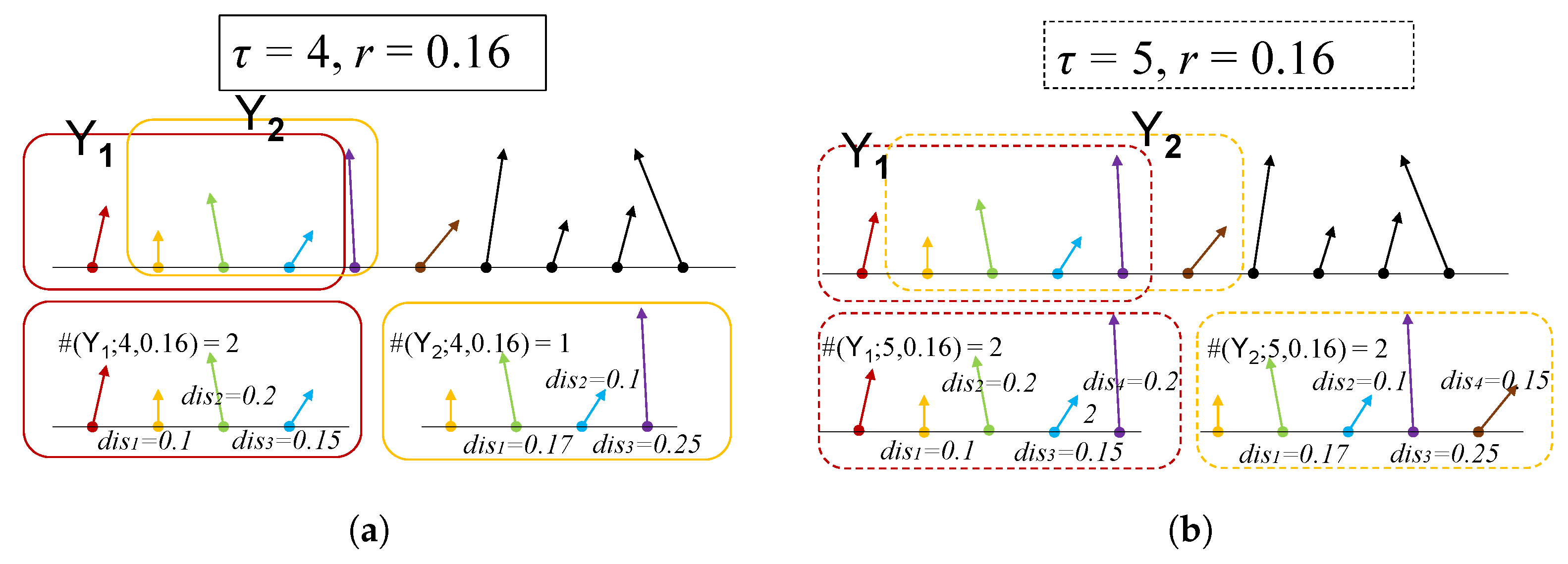
2. Method
3. Numerical Simulations
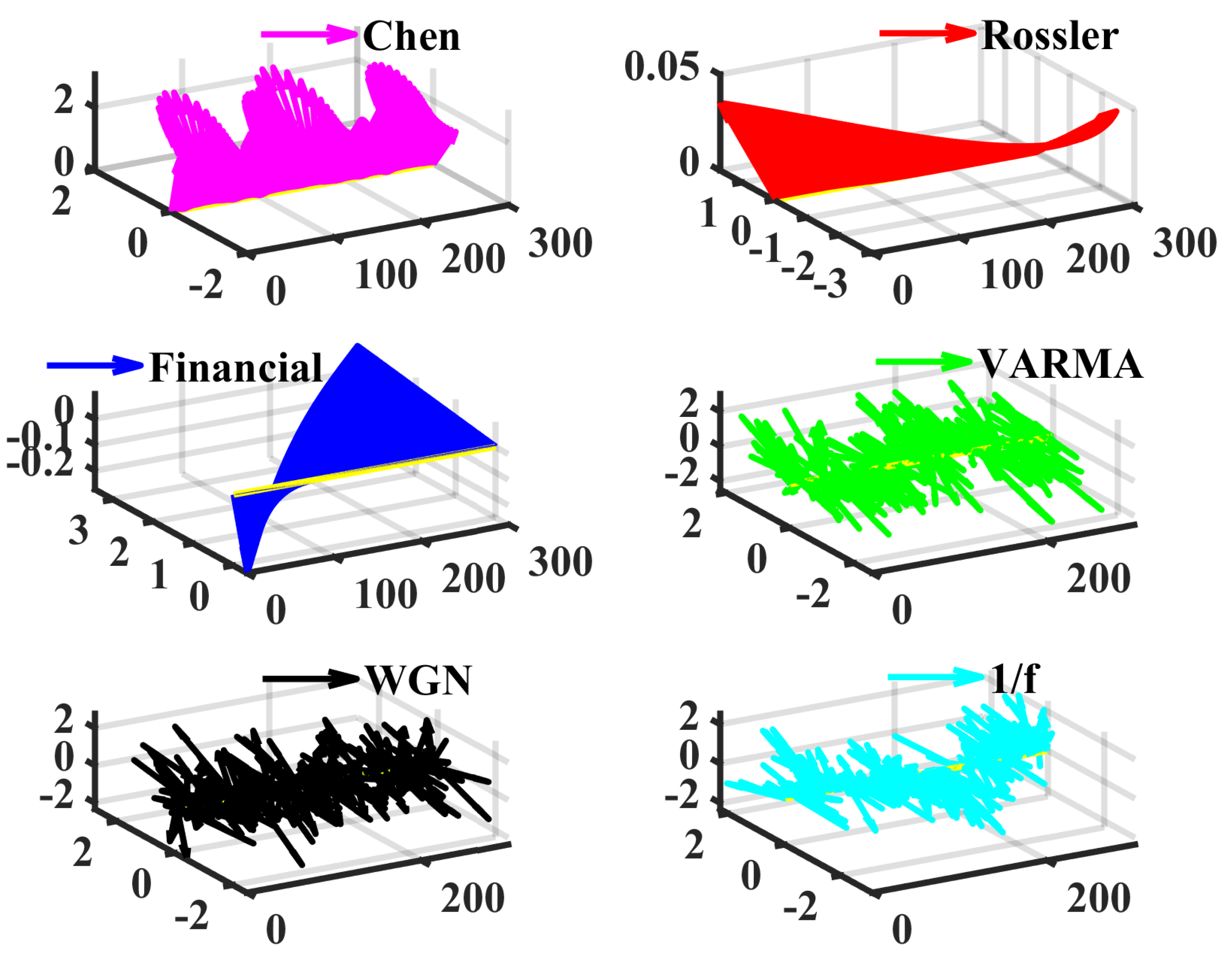
3.1. Fractional-Order Chaotic Systems and Random Series
- Fractional-order Chen system [52], , , , , initial values .
- Fractional-order Rössler system [53], , , , , , .
- Fractional-order financial system [54], , , , , , .
- Multivariate vector autoregression moving-average process, , , , , , covariance matrix is the unit matrix, is a standard Gaussian White noise, and the length equals to the above numerical solutions. This procedure is completed by the ARMA2AR and VARMA function of MATLAB2020b.
- White Gaussian noiseWe use the NORMRND function of MATLAB2020b to simulate WGN (500 × 3). Its components are independent with zero mean and unit standard deviation.
- 1/f noiseOn the basis of the algorithm in [57], the procedure of generating 1/f noise consists of three basic steps: (i) simulating white noise whose length is 1500, we obtain ; (ii) DFT (discrete Fourier transformation) on , multiplied by and symmetrized for a real function, then IDFT (inverse discrete Fourier transformation), adjust the mean and standard deviations, yielding ; (iii) resize and to matrix; finally, the 1/f noise series is composed as .
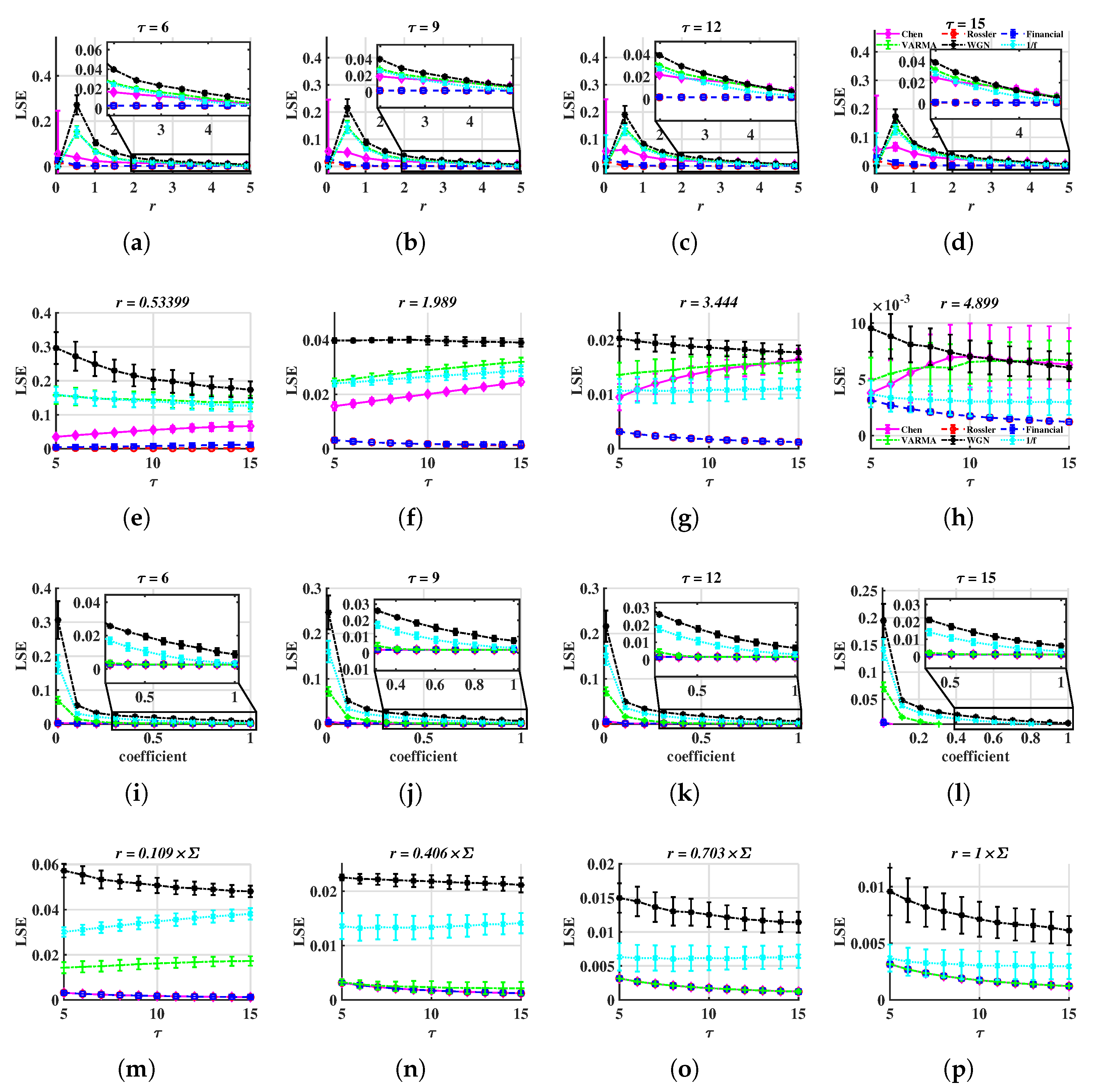
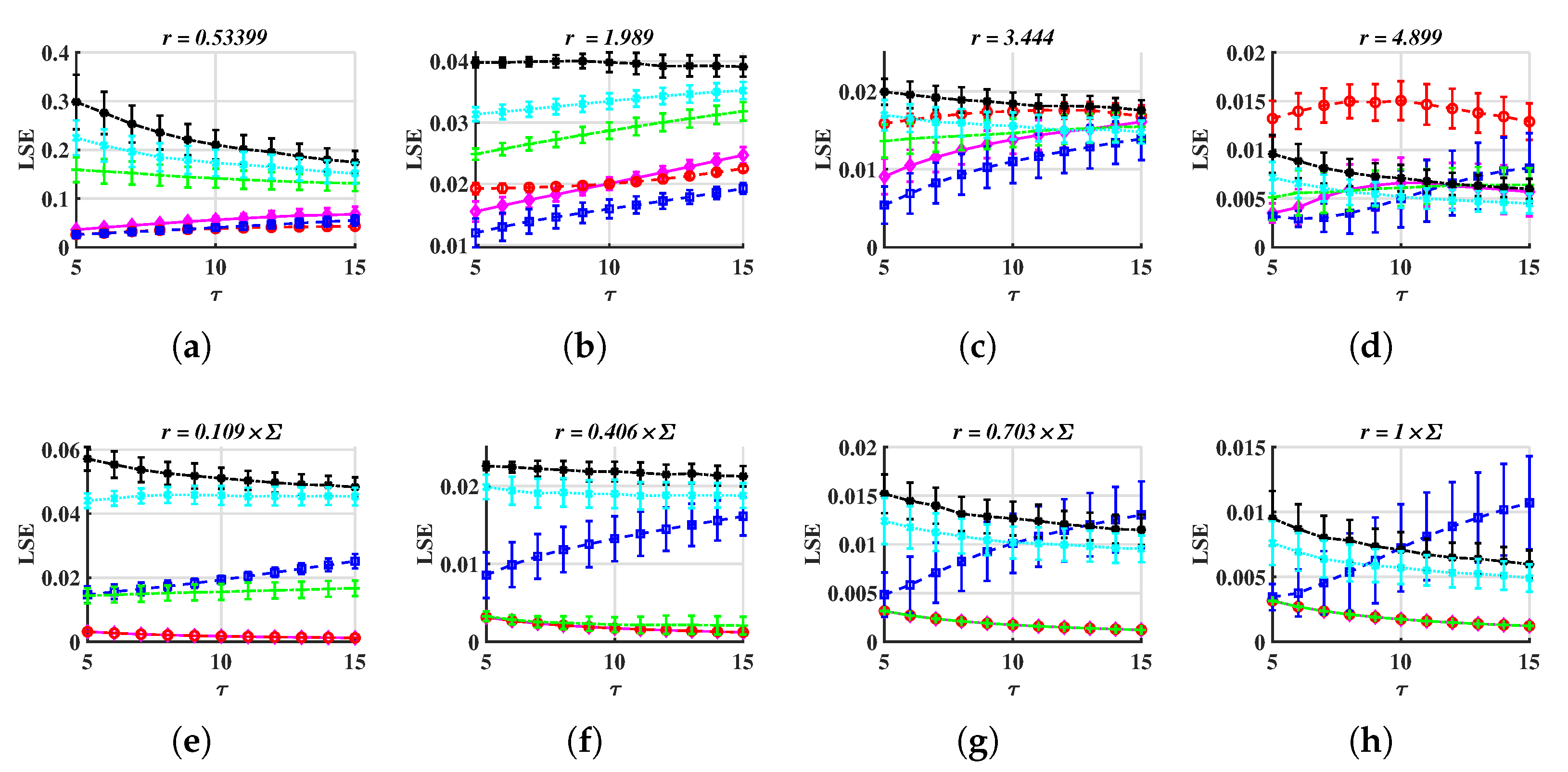
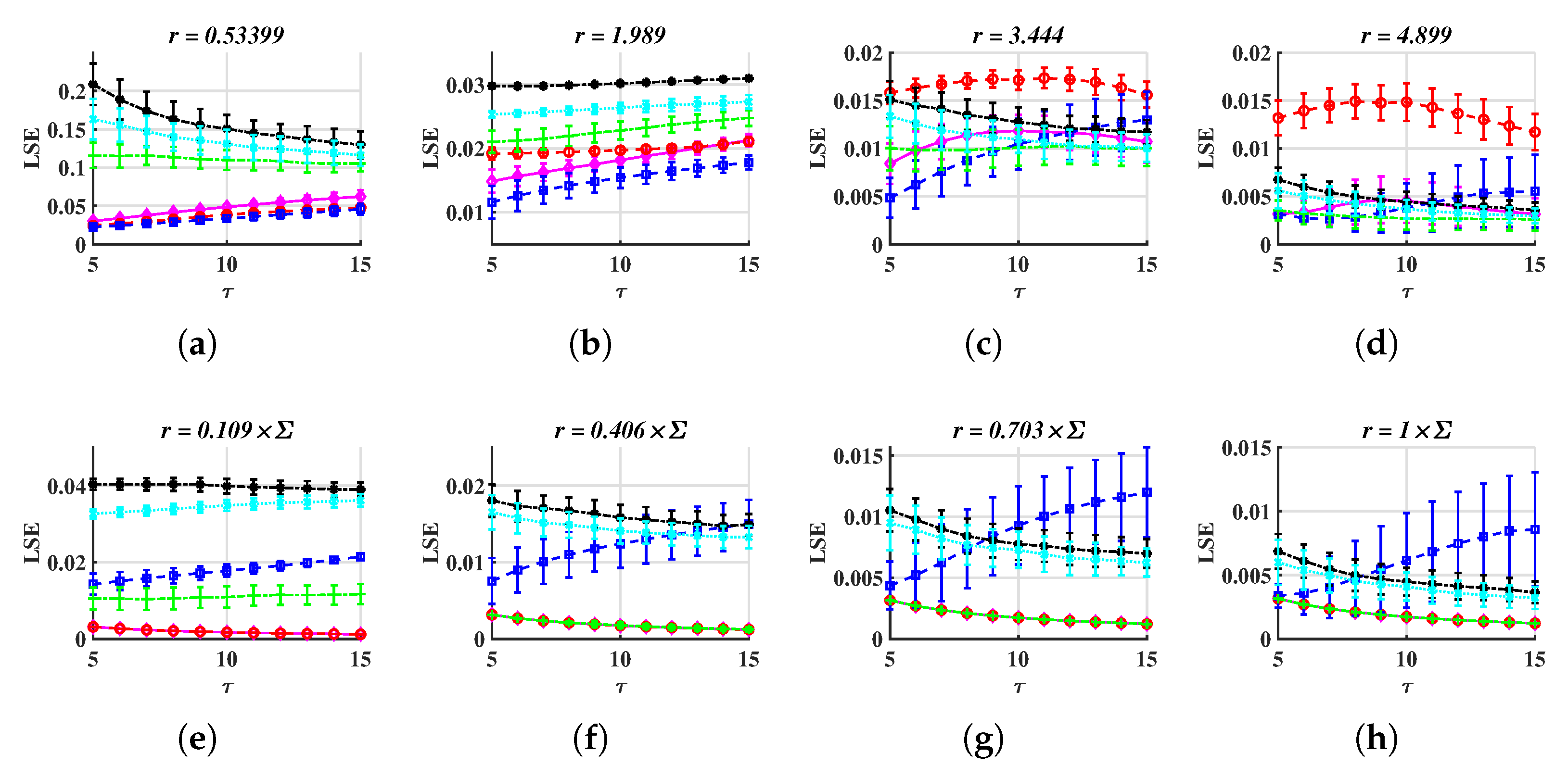
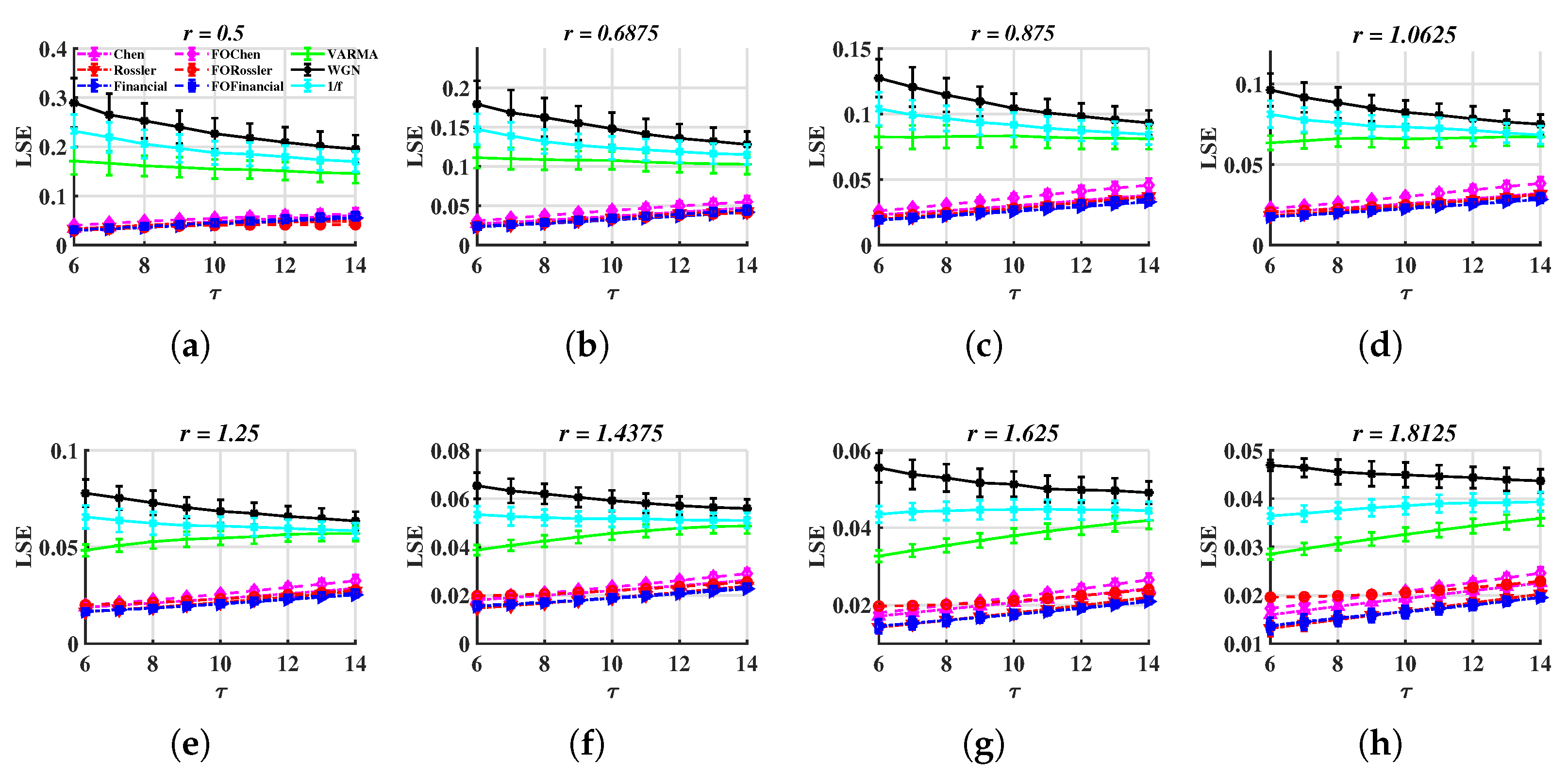
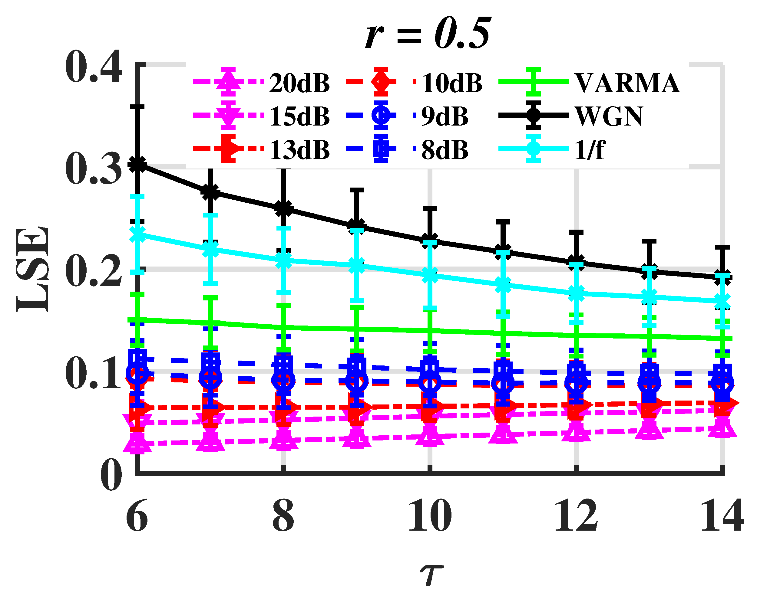
- is acceptable. In Figure 4a–d and in Figure 4i–l, when r is taken appropriately, these curves have essentially the same shape, making it possible to distinguish between different signals. This suggests that the distinction is not dependent on the value of , and the corresponding time complexity can be taken into consideration when designing this parameter.
- For METHOD A, . For METHOD B, . For example, when , is less than 0.1 but is higher than 0.1. Therefore, the stochastic sequence can be distinguished from chaotic ones. See Figure 4e. If r is too small, has a large standard deviation, as is shown in Figure 4a,i. If r is too large, and are overlapped, thus, it is difficult to tell apart various signals. See Figure 4g,o.
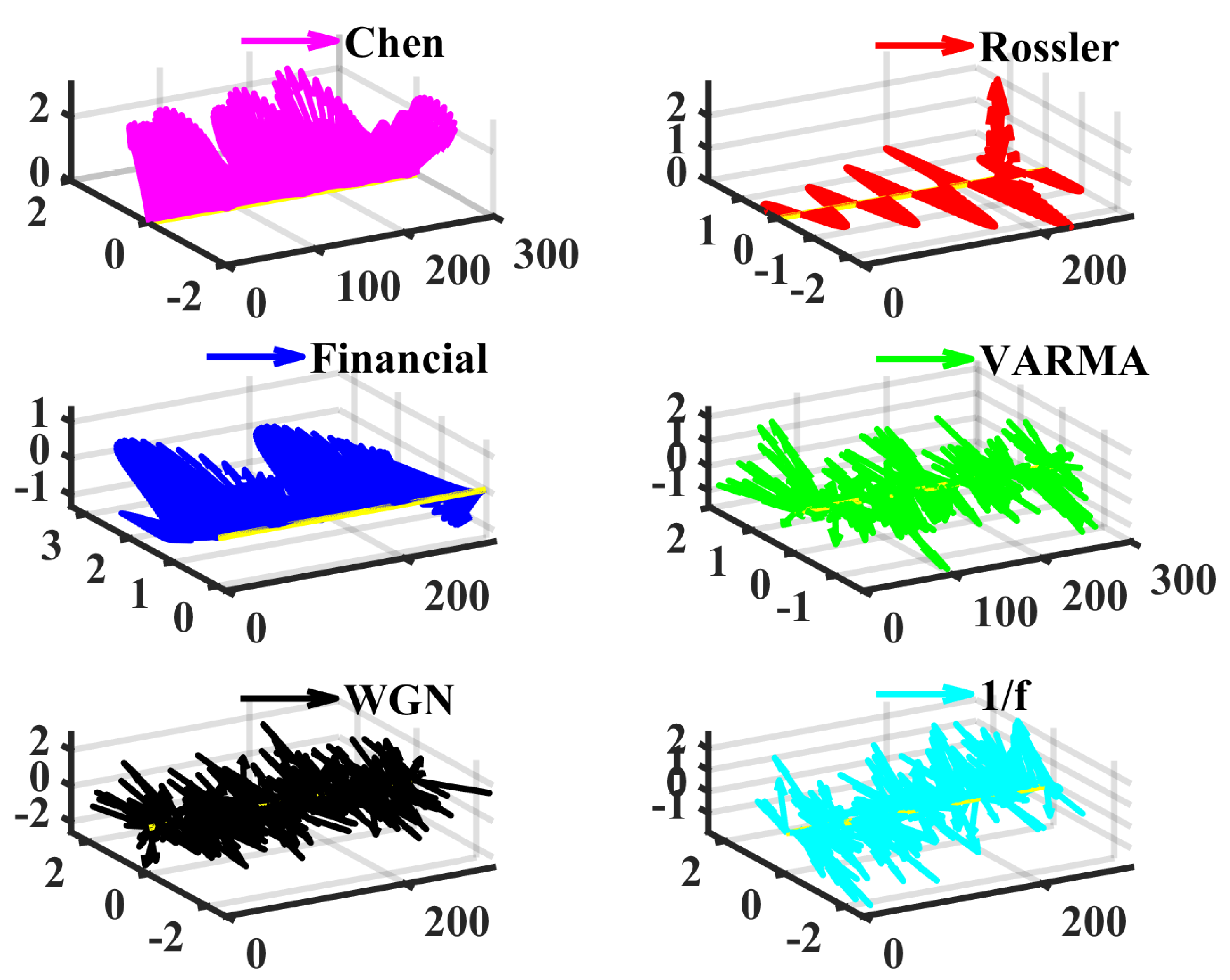
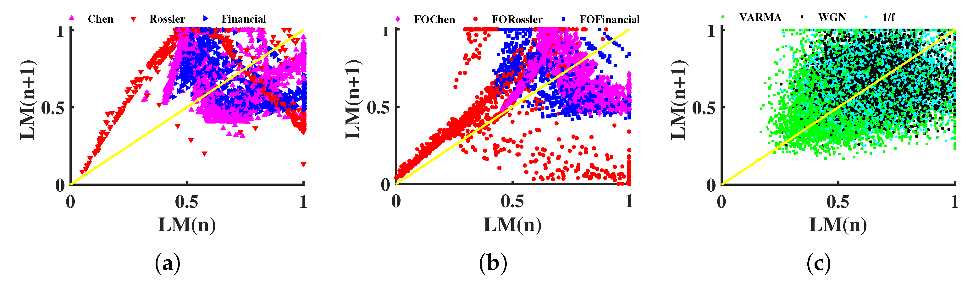
3.2. Integer-Order Chaos, Fractional-Order Chaos, and Random Series
- Integer-order Chen system [52], , , , initial values .
- Integer-order Rössler system [53], , , .
- Integer-order financial system [54], , , .
- Multi-scale entropy and complex networks often necessitate a substantial number of data nodes to obtain useful findings, but LSE can process relatively short time series. The length of the test cases in this section is only 500.
- According to the calculation process in Section 2, it is simple to know that the time complexity of the LSE method is linear () and appropriate for handling real-time jobs.
- LSE is more effective at depicting the short-term autocorrelation and the correlation between various components of multidimensional time series because it takes advantage of the similarity of vectors in sliding windows.
4. Application on Real-World Data
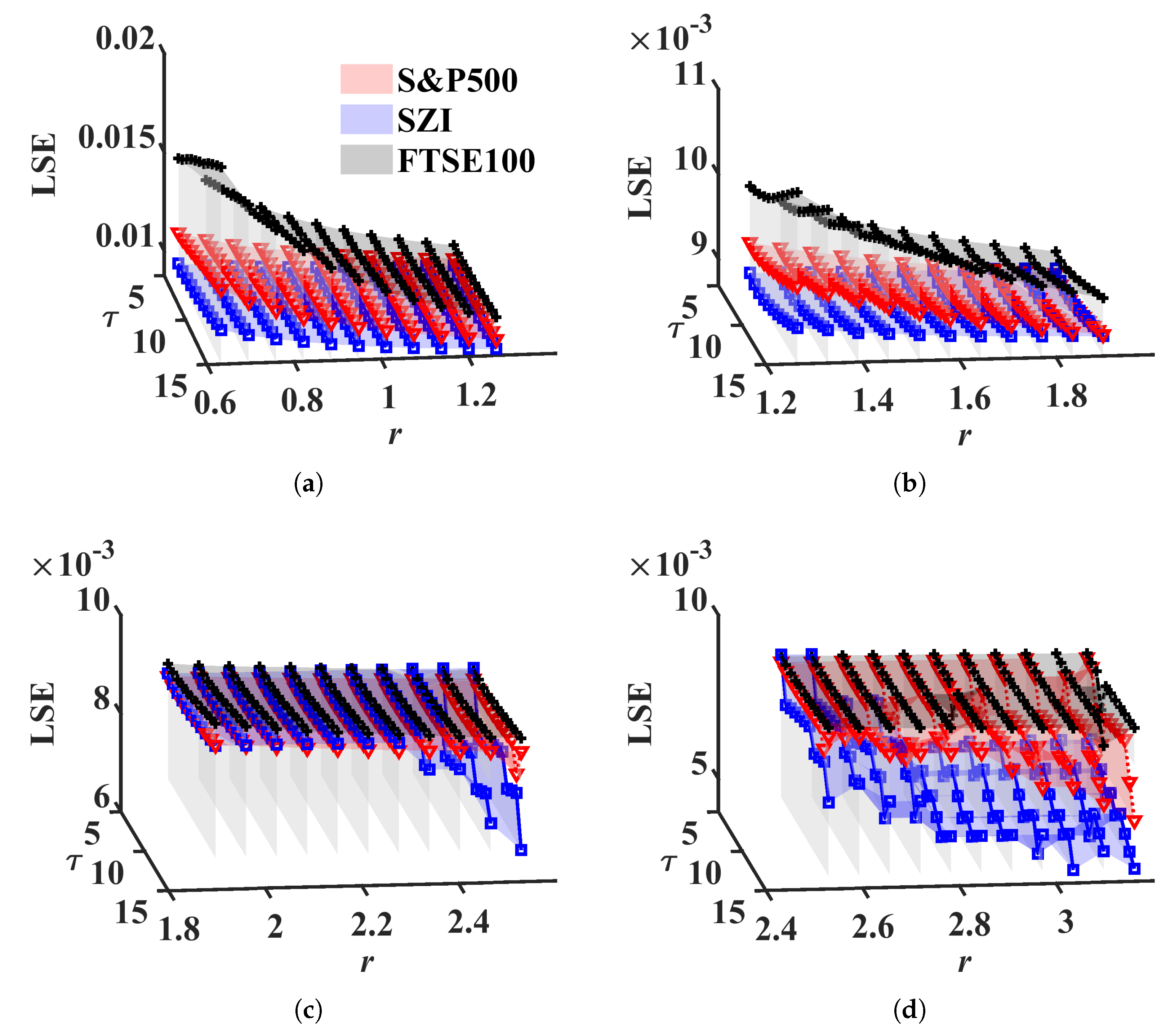
4.1. Financial Market Index
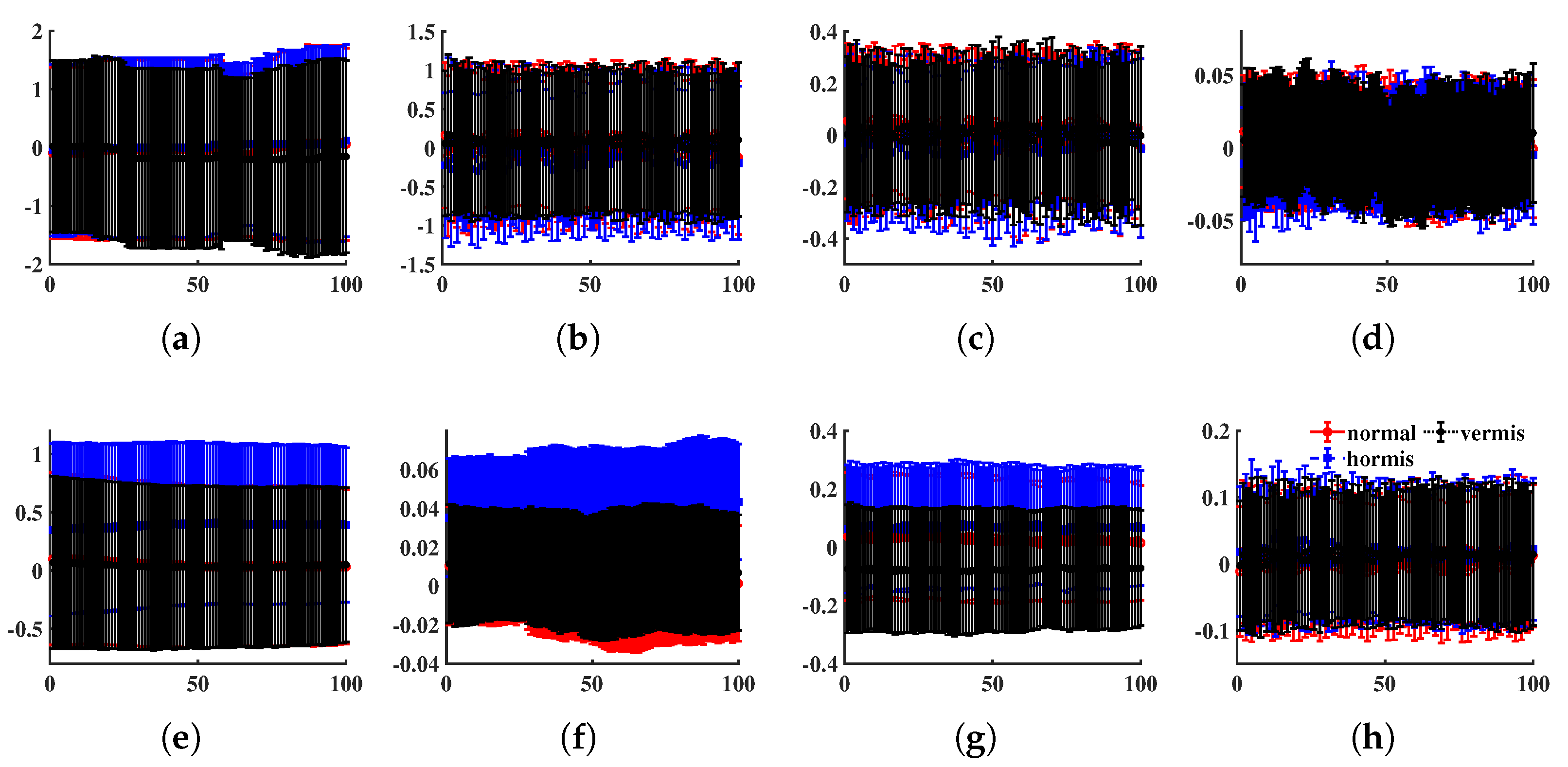
4.2. Machinery Fault Recognition
5. Conclusions
Author Contributions
Funding
Institutional Review Board Statement
Informed Consent Statement
Data Availability Statement
Acknowledgments
Conflicts of Interest
Appendix A
Appendix A.1
Appendix A.2
References
- Sulistiyono, S.; Akhiruyanto, A.; Primasoni, N.; Arjuna, F.; Santoso, N.; Yudhistira, D. The effect of 10 weeks game experience learning (gel) based training on teamwork, respect attitude, skill and physical ability in young football players. Teorìâ ta Metod. Fìzičnogo Vihovannâ 2021, 21, 173–179. [Google Scholar] [CrossRef]
- Follesa, M.; Fragiacomo, M.; Casagrande, D.; Tomasi, R.; Piazza, M.; Vassallo, D.; Canetti, D.; Rossi, S. The new provisions for the seismic design of timber buildings in Europe. Eng. Struct. 2018, 168, 736–747. [Google Scholar] [CrossRef]
- Gao, T.; Fadnis, K.; Campbell, M. Local-to-global Bayesian network structure learning. In Proceedings of the International Conference on Machine Learning, Sydney, Australia, 6–11 August 2017; pp. 1193–1202. [Google Scholar]
- Friedman, N.; Goldszmidt, M. Learning Bayesian networks with local structure. In Learning in Graphical Models; Springer: Berlin/Heidelberg, Germany, 1998; pp. 421–459. [Google Scholar]
- Lei, C.; Zhu, X. Unsupervised feature selection via local structure learning and sparse learning. Multimed. Tools Appl. 2018, 77, 29605–29622. [Google Scholar] [CrossRef]
- Li, J.; Wen, G.; Gan, J.; Zhang, L.; Zhang, S. Sparse nonlinear feature selection algorithm via local structure learning. Emerg. Sci. J. 2019, 3, 115–129. [Google Scholar] [CrossRef] [Green Version]
- Liao, S.; Yi, D.; Lei, Z.; Qin, R.; Li, S.Z. Heterogeneous face recognition from local structures of normalized appearance. In Proceedings of the International Conference on Biometrics, Alghero, Italy, 2–5 June 2009; Springer: Berlin/Heidelberg, Germany, 2009; pp. 209–218. [Google Scholar]
- Qian, J.; Yang, J.; Xu, Y. Local structure-based image decomposition for feature extraction with applications to face recognition. IEEE Trans. Image Process. 2013, 22, 3591–3603. [Google Scholar] [CrossRef] [PubMed]
- Heo, L.; Feig, M. High-accuracy protein structures by combining machine-learning with physics-based refinement. Proteins Struct. Funct. Bioinform. 2020, 88, 637–642. [Google Scholar] [CrossRef] [PubMed]
- Zhang, L.; Du, G.; Liu, F.; Tu, H.; Shu, X. Global-local multiple granularity learning for cross-modality visible-infrared person reidentification. IEEE Trans. Neural Netw. Learn. Syst. 2021. [Google Scholar] [CrossRef]
- Shannon, C.E. A mathematical theory of communication, 1948. Bell Syst. Tech. J. 1948, 27, 3–55. [Google Scholar] [CrossRef] [Green Version]
- Richman, J.S.; Lake, D.E.; Moorman, J.R. Sample entropy. In Methods in Enzymology; Elsevier: Amsterdam, The Netherlands, 2004; Volume 384, pp. 172–184. [Google Scholar]
- Yentes, J.M.; Hunt, N.; Schmid, K.K.; Kaipust, J.P.; McGrath, D.; Stergiou, N. The appropriate use of approximate entropy and sample entropy with short data sets. Ann. Biomed. Eng. 2013, 41, 349–365. [Google Scholar] [CrossRef]
- Costa, M.; Goldberger, A.L.; Peng, C.K. Multiscale entropy analysis of biological signals. Phys. Rev. E 2005, 71, 021906. [Google Scholar] [CrossRef]
- Busa, M.A.; van Emmerik, R.E. Multiscale entropy: A tool for understanding the complexity of postural control. J. Sport Health Sci. 2016, 5, 44–51. [Google Scholar] [CrossRef] [PubMed] [Green Version]
- Bandt, C.; Pompe, B. Permutation entropy: A natural complexity measure for time series. Phys. Rev. Lett. 2002, 88, 174102. [Google Scholar] [CrossRef] [PubMed]
- Keller, K.; Mangold, T.; Stolz, I.; Werner, J. Permutation entropy: New ideas and challenges. Entropy 2017, 19, 134. [Google Scholar] [CrossRef] [Green Version]
- Zhang, Z.; Xiang, Z.; Chen, Y.; Xu, J. Fuzzy permutation entropy derived from a novel distance between segments of time series. AIMS Math. 2020, 5, 6244–6260. [Google Scholar] [CrossRef]
- Morabito, F.C.; Labate, D.; La Foresta, F.; Bramanti, A.; Morabito, G.; Palamara, I. Multivariate multi-scale permutation entropy for complexity analysis of Alzheimer’s disease EEG. Entropy 2012, 14, 1186–1202. [Google Scholar] [CrossRef] [Green Version]
- He, S.; Sun, K.; Wang, H. Multivariate permutation entropy and its application for complexity analysis of chaotic systems. Phys. A Stat. Mech. Its Appl. 2016, 461, 812–823. [Google Scholar] [CrossRef]
- Ying, W.; Tong, J.; Dong, Z.; Pan, H.; Liu, Q.; Zheng, J. Composite multivariate multi-Scale permutation entropy and laplacian score based fault diagnosis of rolling bearing. Entropy 2022, 24, 160. [Google Scholar] [CrossRef]
- Romera, E.; Nagy, Á. Density functional fidelity susceptibility and Kullback–Leibler entropy. Phys. Lett. A 2013, 377, 3098–3101. [Google Scholar] [CrossRef]
- Wang, J.; Zheng, N.; Chen, B.; Chen, P.; Chen, S.; Liu, Z.; Wang, F.Y.; Xi, B. Multivariate Correlation Entropy and Law Discovery in Large Data Sets. IEEE Intell. Syst. 2018, 33, 47–54. [Google Scholar] [CrossRef]
- Yu, S.; Giraldo, L.G.S.; Jenssen, R.; Principe, J.C. Multivariate Extension of Matrix-Based Rényi’s α-Order Entropy Functional. IEEE Trans. Pattern Anal. Mach. Intell. 2019, 42, 2960–2966. [Google Scholar] [CrossRef]
- Wang, Z.; Shang, P. Generalized entropy plane based on multiscale weighted multivariate dispersion entropy for financial time series. Chaos Solitons Fractals 2021, 142, 110473. [Google Scholar] [CrossRef]
- Wang, X.; Si, S.; Li, Y. Variational Embedding Multiscale Diversity Entropy for Fault Diagnosis of Large-Scale Machinery. IEEE Trans. Ind. Electron. 2022, 69, 3109–3119. [Google Scholar] [CrossRef]
- Yin, Y.; Wang, X.; Li, Q.; Shang, P. Generalized multivariate multiscale sample entropy for detecting the complexity in complex systems. Phys. A Stat. Mech. Its Appl. 2020, 545, 123814. [Google Scholar] [CrossRef]
- Berrett, T.B.; Samworth, R.J.; Yuan, M. Efficient multivariate entropy estimation via k-nearest neighbour distances. Ann. Stat. 2019, 47, 288–318. [Google Scholar] [CrossRef] [Green Version]
- Azami, H.; Escudero, J. Refined composite multivariate generalized multiscale fuzzy entropy: A tool for complexity analysis of multichannel signals. Phys. A Stat. Mech. Its Appl. 2017, 465, 261–276. [Google Scholar] [CrossRef] [Green Version]
- Han, Y.F.; Jin, N.D.; Zhai, L.S.; Ren, Y.Y.; He, Y.S. An investigation of oil–water two-phase flow instability using multivariate multi-scale weighted permutation entropy. Phys. A Stat. Mech. Its Appl. 2019, 518, 131–144. [Google Scholar] [CrossRef]
- Mao, X.; Shang, P.; Li, Q. Multivariate multiscale complexity-entropy causality plane analysis for complex time series. Nonlinear Dyn. 2019, 96, 2449–2462. [Google Scholar] [CrossRef]
- Shang, B.; Shang, P. Complexity analysis of multiscale multivariate time series based on entropy plane via vector visibility graph. Nonlinear Dyn. 2020, 102, 1881–1895. [Google Scholar] [CrossRef]
- Barabási, A.L.; Albert, R. Emergence of scaling in random networks. Science 1999, 286, 509–512. [Google Scholar] [CrossRef] [Green Version]
- Cong, J.; Liu, H. Approaching human language with complex networks. Phys. Life Rev. 2014, 11, 598–618. [Google Scholar] [CrossRef]
- Ruths, J.; Ruths, D. Control profiles of complex networks. Science 2014, 343, 1373–1376. [Google Scholar] [CrossRef] [PubMed]
- Albert, R.; Jeong, H.; Barabási, A.L. Error and attack tolerance of complex networks. Nature 2000, 406, 378–382. [Google Scholar] [CrossRef] [PubMed] [Green Version]
- Donges, J.F.; Zou, Y.; Marwan, N.; Kurths, J. Complex networks in climate dynamics. Eur. Phys. J. Spec. Top. 2009, 174, 157–179. [Google Scholar] [CrossRef] [Green Version]
- Mutua, S.; Gu, C.; Yang, H. Visibility graphlet approach to chaotic time series. Chaos 2016, 26, 053107. [Google Scholar] [CrossRef]
- Marwan, N.; Kurths, J. Complex network based techniques to identify extreme events and (sudden) transitions in spatio-temporal systems. Chaos 2015, 25, 097609. [Google Scholar] [CrossRef] [Green Version]
- Zhang, Z.; Xu, J.; Zhou, X. Mapping time series into complex networks based on equal probability division. AIP Adv. 2019, 9, 015017. [Google Scholar] [CrossRef] [Green Version]
- Zhao, Y.; Peng, X.; Small, M. Reciprocal characterization from multivariate time series to multilayer complex networks. Chaos 2020, 30, 013137. [Google Scholar] [CrossRef]
- Small, M.; Zhang, J.; Xu, X. Transforming time series into complex networks. Lect. Notes Inst. Comput. Sci. Soc. Telecommun. Eng. 2009, 5 LNICST, 2078–2089. [Google Scholar] [CrossRef]
- Silva, V.F.; Silva, M.E.; Ribeiro, P.; Silva, F. Time series analysis via network science: Concepts and algorithms. Wiley Interdiscip. Rev. Data Min. Knowl. Discov. 2021, 11, e1404. [Google Scholar] [CrossRef]
- Lacasa, L.; Luque, B.; Ballesteros, F.; Luque, J.; Nuno, J.C. From time series to complex networks: The visibility graph. Proc. Natl. Acad. Sci. USA 2008, 105, 4972–4975. [Google Scholar] [CrossRef]
- Lacasa, L.; Just, W. Visibility graphs and symbolic dynamics. Phys. D Nonlinear Phenom. 2018, 374–375, 35–44. [Google Scholar] [CrossRef] [Green Version]
- Donner, R.V.; Small, M.; Donges, J.F.; Marwan, N.; Zou, Y.; Xiang, R.; Kurths, J. Recurrence-based time series analysis by means of complex network methods. Int. J. Bifurc. Chaos 2011, 21, 1019–1046. [Google Scholar] [CrossRef]
- Donges, J.F.; Heitzig, J.; Donner, R.V.; Kurths, J. Analytical framework for recurrence network analysis of time series. Phys. Rev. E 2012, 85, 046105. [Google Scholar] [CrossRef] [PubMed] [Green Version]
- Ruan, Y.; Donner, R.V.; Guan, S.; Zou, Y. Ordinal partition transition network based complexity measures for inferring coupling direction and delay from time series. Chaos Interdiscip. J. Nonlinear Sci. 2019, 29, 043111. [Google Scholar] [CrossRef]
- Guo, H.; Zhang, J.Y.; Zou, Y.; Guan, S.G. Cross and joint ordinal partition transition networks for multivariate time series analysis. Front. Phys. 2018, 13, 130508. [Google Scholar] [CrossRef] [Green Version]
- Donner, R.V.; Zou, Y.; Donges, J.F.; Marwan, N.; Kurths, J. Recurrence networks—A novel paradigm for nonlinear time series analysis. New J. Phys. 2010, 12, 033025. [Google Scholar] [CrossRef] [Green Version]
- Cattani, C.; Srivastava, H.M.; Yang, X.J. Fractional Dynamics; Walter de Gruyter GmbH & Co KG: Berlin, Germany, 2015; pp. 166–173. [Google Scholar]
- Li, C.; Chen, G. Chaos in the fractional order Chen system and its control. Chaos Solitons Fractals 2004, 22, 549–554. [Google Scholar] [CrossRef]
- Zhang, W.; Zhou, S.; Li, H.; Zhu, H. Chaos in a fractional-order Rössler system. Chaos Solitons Fractals 2009, 42, 1684–1691. [Google Scholar] [CrossRef]
- Chen, W.C. Nonlinear dynamics and chaos in a fractional-order financial system. Chaos Solitons Fractals 2008, 36, 1305–1314. [Google Scholar] [CrossRef]
- Podlubny, I. An introduction to fractional derivatives, fractional differential equations, to methods of their solution and some of their applications. Math. Sci. Eng. 1999, 198, 340. [Google Scholar]
- Petráš, I. Fractional-Order Nonlinear Systems: Modeling, Analysis and Simulation; Springer Science & Business Media: New York, NY, USA, 2011; pp. 285–290. [Google Scholar]
- Zhivomirov, H. A method for colored noise generation. Rom. J. Acoust. Vib. 2018, 15, 14–19. [Google Scholar]
- Ouyang, G.; Li, J.; Liu, X.; Li, X. Dynamic characteristics of absence EEG recordings with multiscale permutation entropy analysis. Epilepsy Res. 2013, 104, 246–252. [Google Scholar] [CrossRef] [PubMed]
- Mukherjee, S.; Zawar-Reza, P.; Sturman, A.; Mittal, A.K. Characterizing atmospheric surface layer turbulence using chaotic return map analysis. Meteorol. Atmos. Phys. 2013, 122, 185–197. [Google Scholar] [CrossRef]
- Chidori, K.; Yamamoto, Y. Effects of the lateral amplitude and regularity of upper body fluctuation on step time variability evaluated using return map analysis. PloS ONE 2017, 12, e0180898. [Google Scholar] [CrossRef] [Green Version]
- Rybin, V.; Butusov, D.; Rodionova, E.; Karimov, T.; Ostrovskii, V.; Tutueva, A. Discovering chaos-based communications by recurrence quantification and quantified return map analyses. Int. J. Bifurc. Chaos 2022, 32, 2250136. [Google Scholar] [CrossRef]
- Voznesensky, A.; Butusov, D.; Rybin, V.; Kaplun, D.; Karimov, T.; Nepomuceno, E. Denoising Chaotic Signals using Ensemble Intrinsic Time-Scale Decomposition. IEEE Access 2022. Available online: https://ieeexplore.ieee.org/abstract/document/9932609 (accessed on 20 November 2022).
- Yahoo. Yahoo Finance. Available online: https://www.yahoo.com/author/yahoo-finance (accessed on 6 June 2022).
- Cao, H.; Li, Y. Unraveling chaotic attractors by complex networks and measurements of stock market complexity. Chaos Interdiscip. J. Nonlinear Sci. 2014, 24, 013134. [Google Scholar] [CrossRef]
- Ribeiro, F.M.L. MAFAULDA—Machinery Fault Database [Online]. 2021. Available online: http://www02.smt.ufrj.br/~offshore/mfs/page_01.html (accessed on 15 July 2022).
- Song, Y.Y.; Ying, L. Decision tree methods: Applications for classification and prediction. Shanghai Arch. Psychiatry 2015, 27, 130. [Google Scholar]
- Ren, G.; Wang, Y.; Ning, J.; Zhang, Z. Using near-infrared hyperspectral imaging with multiple decision tree methods to delineate black tea quality. Spectrochim. Acta Part A Mol. Biomol. Spectrosc. 2020, 237, 118407. [Google Scholar] [CrossRef]
- Himeur, Y.; Alsalemi, A.; Bensaali, F.; Amira, A. Robust event-based non-intrusive appliance recognition using multi-scale wavelet packet tree and ensemble bagging tree. Appl. Energy 2020, 267, 114877. [Google Scholar] [CrossRef]


| Index | Length | Region |
|---|---|---|
| S&P500 | 1256 | American |
| SZI | 1220 | China |
| FTSE 100 | 1263 | Europe |
Publisher’s Note: MDPI stays neutral with regard to jurisdictional claims in published maps and institutional affiliations. |
© 2022 by the authors. Licensee MDPI, Basel, Switzerland. This article is an open access article distributed under the terms and conditions of the Creative Commons Attribution (CC BY) license (https://creativecommons.org/licenses/by/4.0/).
Share and Cite
Zhang, Z.; Wu, J.; Chen, Y.; Wang, J.; Xu, J. Distinguish between Stochastic and Chaotic Signals by a Local Structure-Based Entropy. Entropy 2022, 24, 1752. https://doi.org/10.3390/e24121752
Zhang Z, Wu J, Chen Y, Wang J, Xu J. Distinguish between Stochastic and Chaotic Signals by a Local Structure-Based Entropy. Entropy. 2022; 24(12):1752. https://doi.org/10.3390/e24121752
Chicago/Turabian StyleZhang, Zelin, Jun Wu, Yufeng Chen, Ji Wang, and Jinyu Xu. 2022. "Distinguish between Stochastic and Chaotic Signals by a Local Structure-Based Entropy" Entropy 24, no. 12: 1752. https://doi.org/10.3390/e24121752