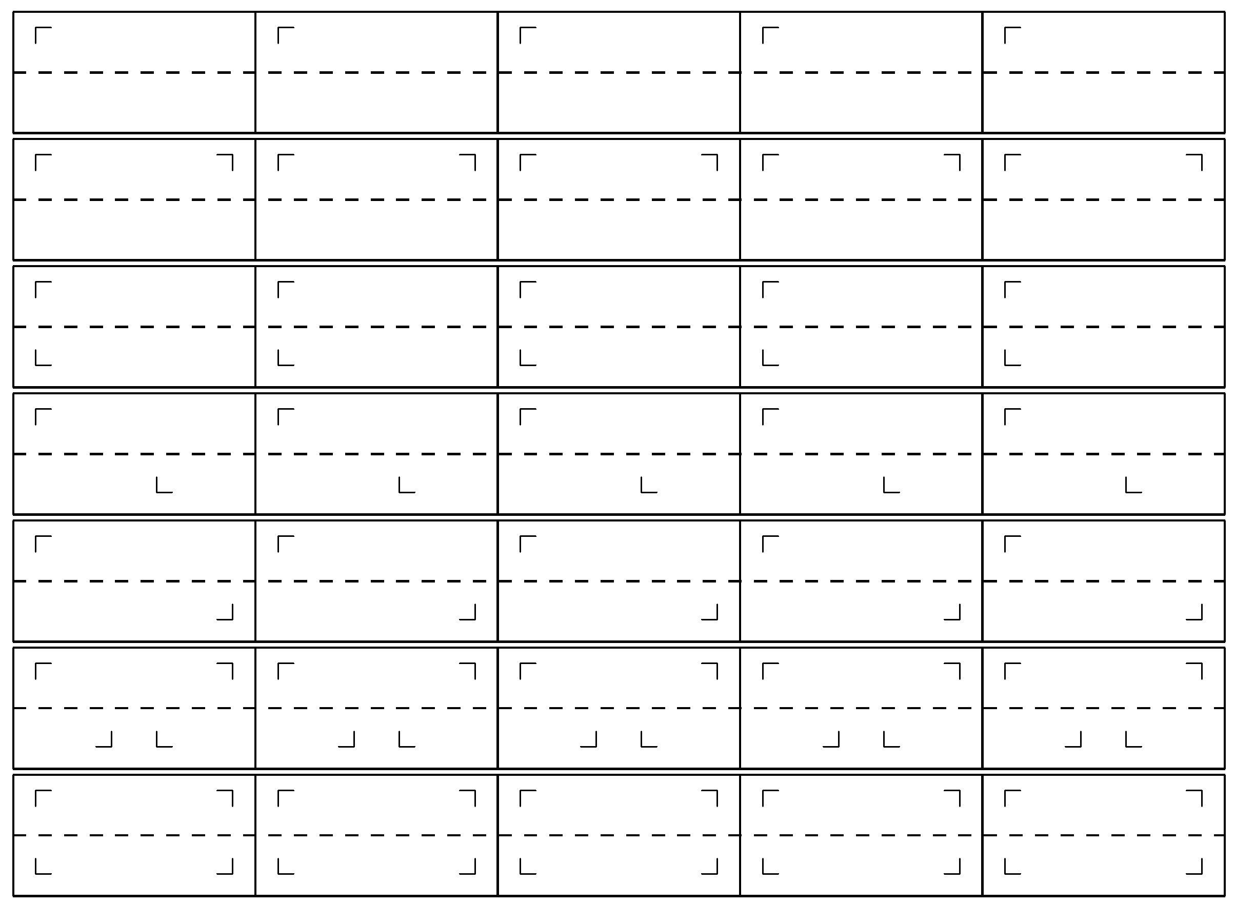
Figure 1.
The seven types of friezes with a ⌜ pattern. The friezes 1, 2, 4, 5 and 6 can constitute periodic discrete sequences because no pattern appears with the same abscissa. This is not the case for friezes 3 and 7, which cannot constitute a discrete sequence. Among the five periodic sequences, friezes 2 and 6 are composed of palindromes.
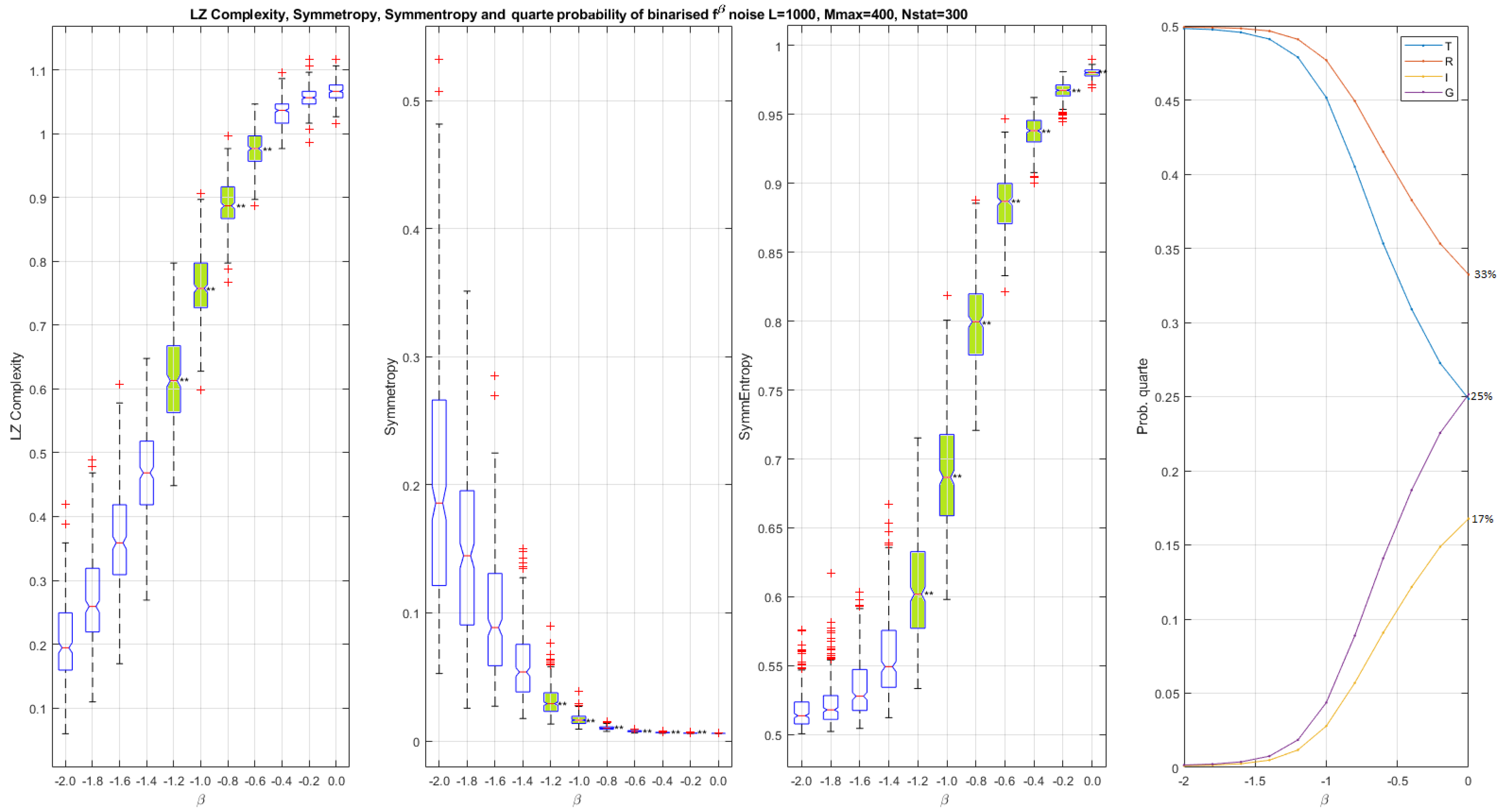
Figure 2.
Scalar palindromic descriptors obtained from binarized noises and for different values of . Left, Lempel–Ziv complexity , in which the boxes do not overlap for . Left middle, symmetropy , in which the boxes do not overlap for . Right middle, symmentropy , in which boxes do not overlap for . Left, quarte probability versus . When , the quarte probability is . When , the quarte probability is and the level of reflection symmetry is higher than the translation/ glide reflection and the inversion: . The closer is to zero, the higher the complexity. We notice that both and increase as the complexity increases. On the contrary decreases as the complexity increases.
Figure 3.
Average palindromic vectors obtained for binarized noises of length 1000, with (from top to bottom) and . Top, average palindromic vectors obtained after averaging 300 vectors for . Middle, average palindromic vectors obtained after averaging 300 vectors for . Bottom, average palindrome vectors obtained after averaging 300 vectors for . The more irregular the sequence (strong negative value of ) and the larger the spread of the palindromic vector descriptors.
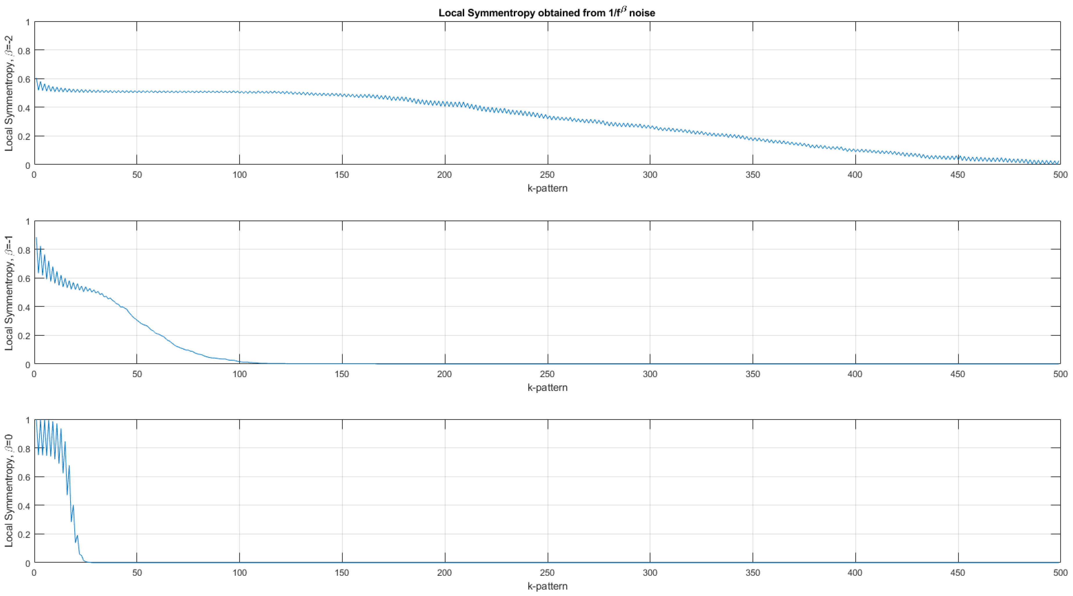
Figure 4.
Average local symmentropy (with 300 trials) computed for three types of noises. Top, local symmentropy of a Brownian motion (). Middle, local symmentropy of a pink noise (). Bottom, local symmentropy of a white noise (). The sawtooth fluctuation comes from the fact that the symmentropy values are slightly different for even and odd palindromes. The local symmentropy synthesizes the information carried by the four palindromic vectors into only one.
Figure 5.
Logarithm of the four average palindromic vectors computed from 100 binary sequences iid (independent and identically distributed) of 5000 bits. We note a different distribution between even and odd palindromes. There is an equi-distribution between the different types of symmetry for even palindromes. For odd palindromes, we also note the non-presence of palindromes of ‘I’ type. We note a decrease in the symmetry levels as the size of the palindromes increases. Note that there are no palindromes with sizes exceeding 40. Finally, on average, the proportion of palindromes is and .
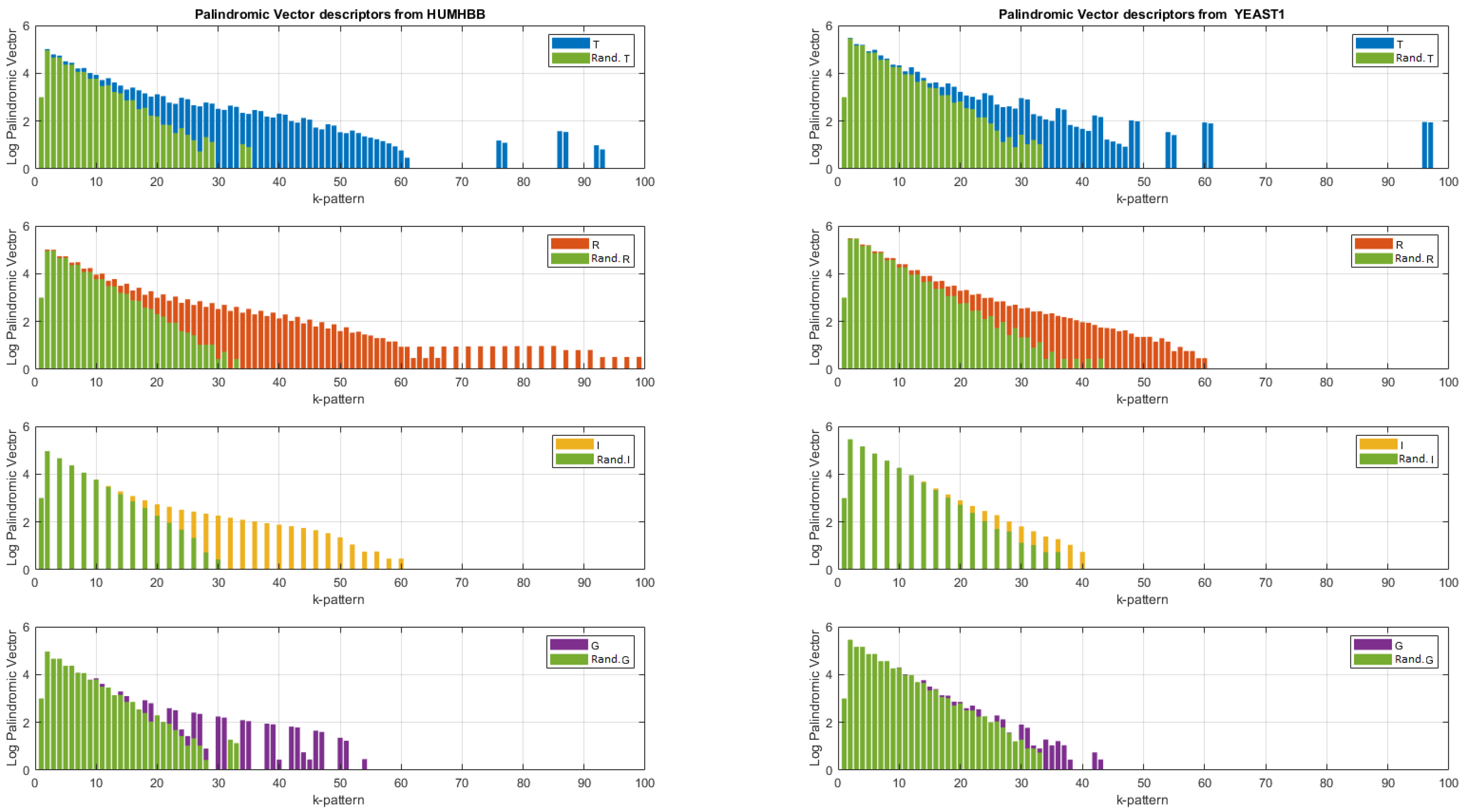
Figure 6.
Logarithm of the palindromic vectors obtained from the entirety of the two DNA sequences for . Zoom for . In green, logarithm of the palindromic vectors obtained after randomization of the DNA sequences.
Figure 6.
Logarithm of the palindromic vectors obtained from the entirety of the two DNA sequences for . Zoom for . In green, logarithm of the palindromic vectors obtained after randomization of the DNA sequences.
Figure 7.
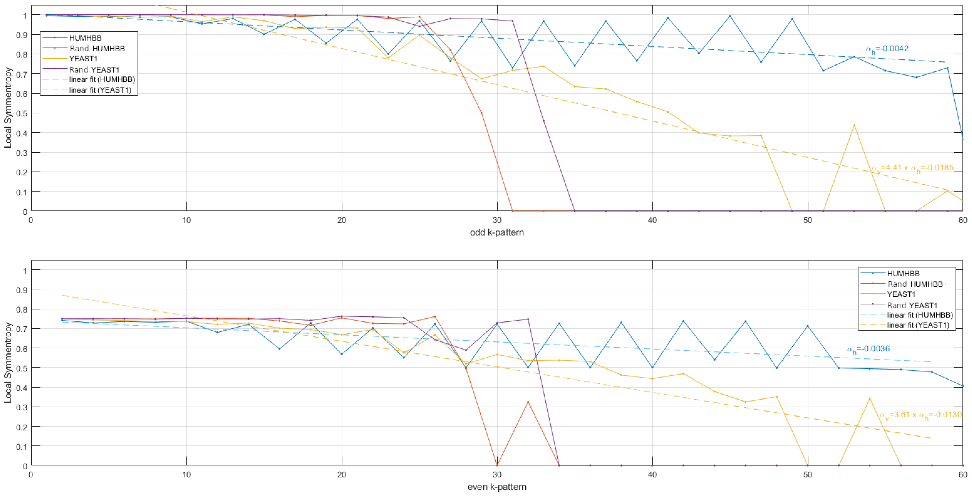
Local symmentropies obtained from binarized DNA sequences in the scale range . Top, odd palindromes. In blue, local symmentropy obtained from HUMHBB and straight line fitting. In orange, local symmentropy obtained from YEAST1 and straight line fitting. In magenta, local symmentropy obtained from randomized HUMHBB. In red, local symmentropy obtained from randomized Yeast. The slope derived from the linear fitting for YEAST1 is times the slope obtained from HUMHBB. Bottom, even palindromes. The slope derived from the linear fitting for YEAST1 is times the slope obtained from HUMHBB.
Figure 7.
Local symmentropies obtained from binarized DNA sequences in the scale range . Top, odd palindromes. In blue, local symmentropy obtained from HUMHBB and straight line fitting. In orange, local symmentropy obtained from YEAST1 and straight line fitting. In magenta, local symmentropy obtained from randomized HUMHBB. In red, local symmentropy obtained from randomized Yeast. The slope derived from the linear fitting for YEAST1 is times the slope obtained from HUMHBB. Bottom, even palindromes. The slope derived from the linear fitting for YEAST1 is times the slope obtained from HUMHBB.
Table 1.
, and calculated from the binary sequence composed of bits. There are in total sizes of palindromes () derived from the dictionary and used in the binary sequence . There are two palindromes of size 2, two palindromes of size 3, and two palindromes of size 4, so a total of palindromes composing the binary sequence.
| m | 0 | 1 | 2 | 3 | 4 | 5 | 6 | 7 | 8 |
|---|
| e | 0,1 | 00,11 | 101,010 | 0110,1001 | - | - | - | - |
| 1 | 2 | 2 | 2 | 2 | 0 | 0 | 0 | 0 |
| 8 | 8 | 2 | 2 | 2 | 0 | 0 | 0 | 0 |
Table 2.
, , and with computed from the 8 binary sequence . The non-trivial palindromic symmetropy is with , , and , and the global palindromic symmentropy is .
Table 2.
, , and with computed from the 8 binary sequence . The non-trivial palindromic symmetropy is with , , and , and the global palindromic symmentropy is .
| m | 0 | 1 | 2 | 3 | 4 | 5 | 6 | 7 | 8 |
|---|
| e | 0,1 | 00,11 | - | 1010 | - | - | - | - |
| 8 | 8 | 2 | 0 | 1 | 0 | 0 | 0 | 0 |
| - | - | | | | | | | |
| - | - | 2/14 | 0 | 1/6 | - | 0 | - | 0 |
| e | 0,1 | 00,11 | 101,010 | 0110,1001 | - | - | - | - |
| 8 | 8 | 2 | 2 | 2 | 0 | 0 | 0 | 0 |
| - | - | | | | | | | |
| - | - | 2/14 | 1/2 | 2/6 | - | 0 | - | 0 |
| e | 0,1 | 01,10 | - | 1010 | - | 110100 | - | 01101001 |
| 8 | 8 | 5 | 0 | 1 | 0 | 1 | 0 | 1 |
| - | - | | | | | | | |
| - | - | 5/14 | 0 | 1/6 | - | 1 | 0 | 1/2 |
| e | 0,1 | 01,10 | 010,101 | 0110,1001 | - | - | - | 01101001 |
| 8 | 8 | 5 | 2 | 2 | 0 | 0 | 0 | 1 |
| - | - | | | | | | | |
| - | - | 5/14 | 1/2 | 2/6 | - | 0 | - | 1/2 |
| - | - | 0.93 | 0.50 | 0.96 | - | 0 | - | 0.50 |
Table 3.
Distribution in % of the total number of palindromes of different types present in each of the two non-randomized and randomized DNA sequences, . For the non-randomized sequences, the most frequent palindromes are reflection palindromes with , while for the randomized sequences, the distribution is . The distribution of the different types of palindromes is very similar regardless of the type of DNA sequence. The differences between the total number of palindromes from non-randomized and randomized HUMHBB and YEAST1 sequences are 496,028 − 441,299 = 54,729 and 1,463,633 − 1,384,396 = 79,237, respectively.
| DNA seq | | | | | |
|---|
| HUMHBB | 29.5% | 36.8% | 13.5% | 20.2% | 496,028 |
| randomized HUMHBB | 24.9% | 33.3% | 16.7% | 25.1% | 441,299 |
| Yeast1 | 27.9% | 35.5% | 14.5% | 22.1% | 1 463 633 |
| randomized Yeast1 | 25.0% | 33.3% | 16.7% | 25.0% | 1,384,396 |
Table 4.
Scalar palindromic descriptors of binarized DNA sequences. Lempel–Ziv complexity , symmentropy and symmetropy with . From scalar palindromic descriptors, it seems possible to differentiate the 2 DNA sequences. The values of Lempel–Ziv complexity and symmentropy are close to unity, indicating a high level of complexity. For randomized DNA sequences, Lempel–Ziv complexity and symmentropy tend toward unity.
| DNA seq | | | |
|---|
| HUMHHB | 0.94 | 0.96 | 0.85 |
| randomized HUMHHB | 1.02 | 0.98 | 0.75 |
| Yeast1 | 0.98 | 0.97 | 0.80 |
| randomized Yeast1 | 1.01 | 0.98 | 0.75 |


