
Stochastic Chaos and Markov Blankets

 , and
, and 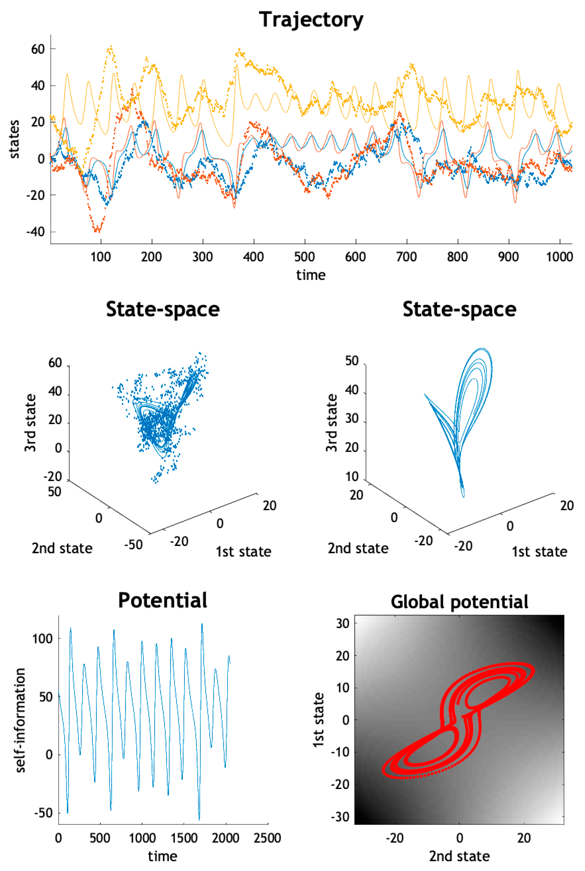
Abstract
:1. Introduction
2. From Dynamics to Densities
3. The Helmholtz Decomposition
3.1. Functional Forms
3.2. The Lorenz System Revisited
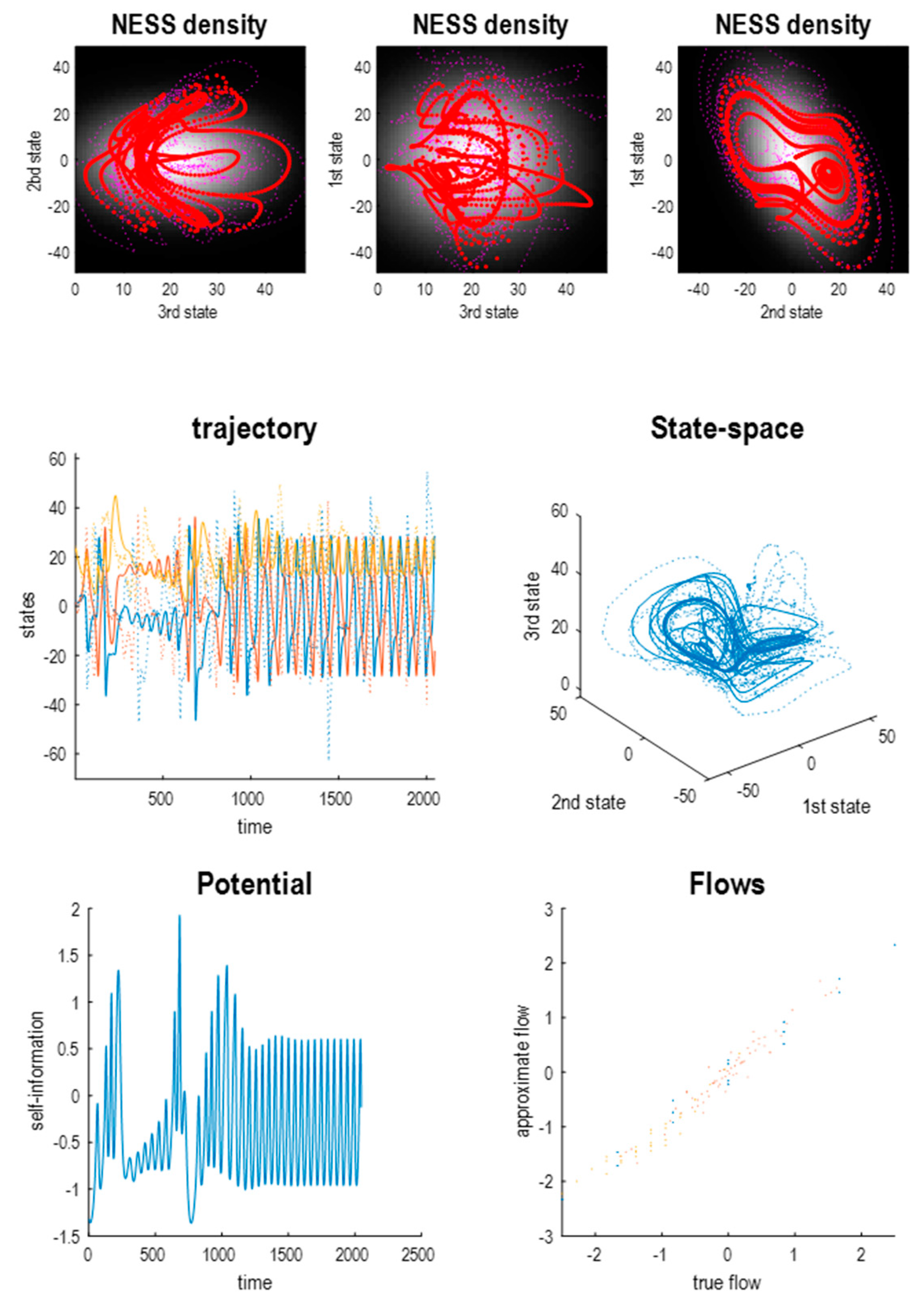
3.3. Beyond the Lorenz System
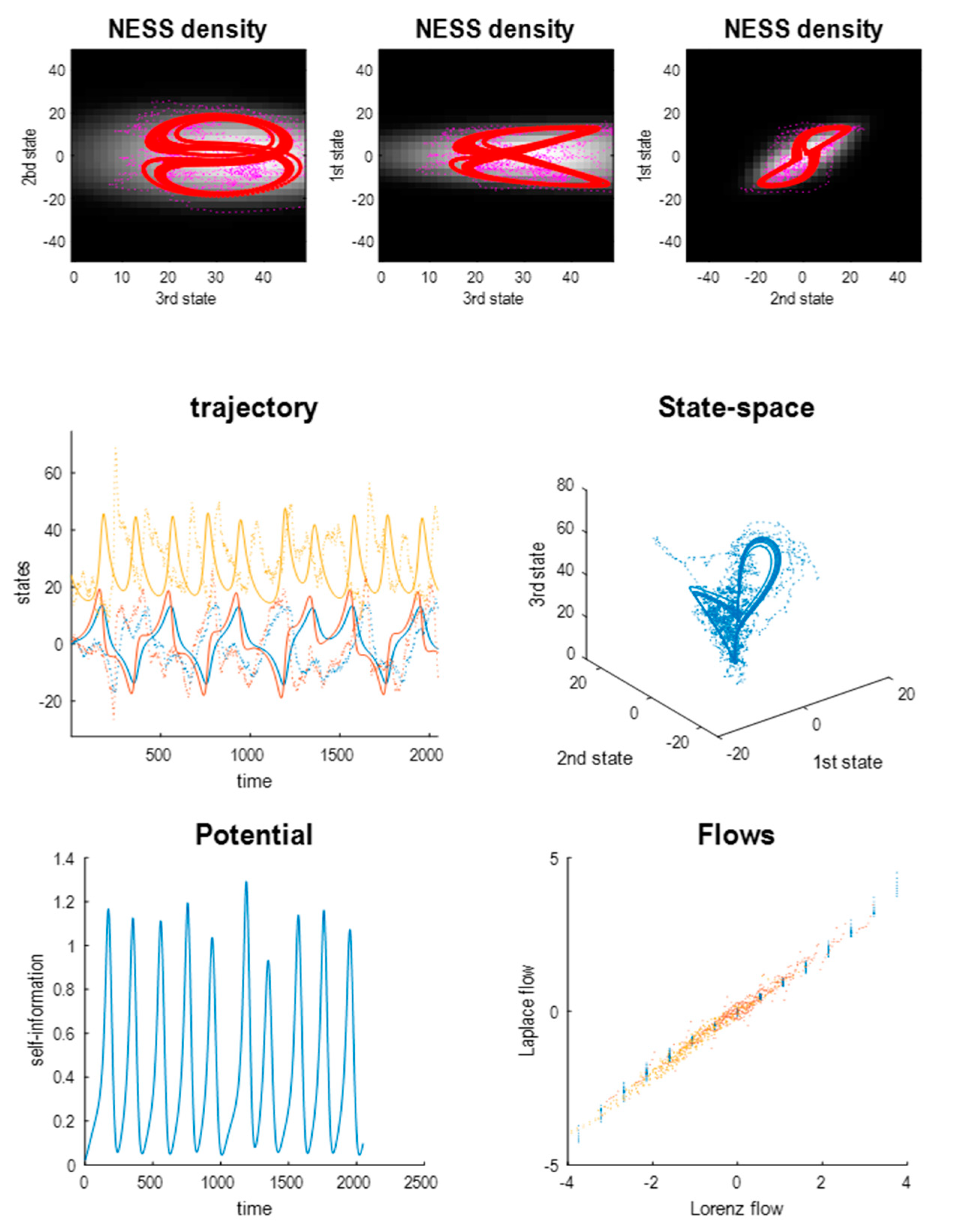
3.4. Beyond the Laplace System
3.5. Summary
4. Markov Blankets and the Free Energy Principle
4.1. Sparsely Coupled Systems
4.2. Particular Partitions, Boundaries and Blankets
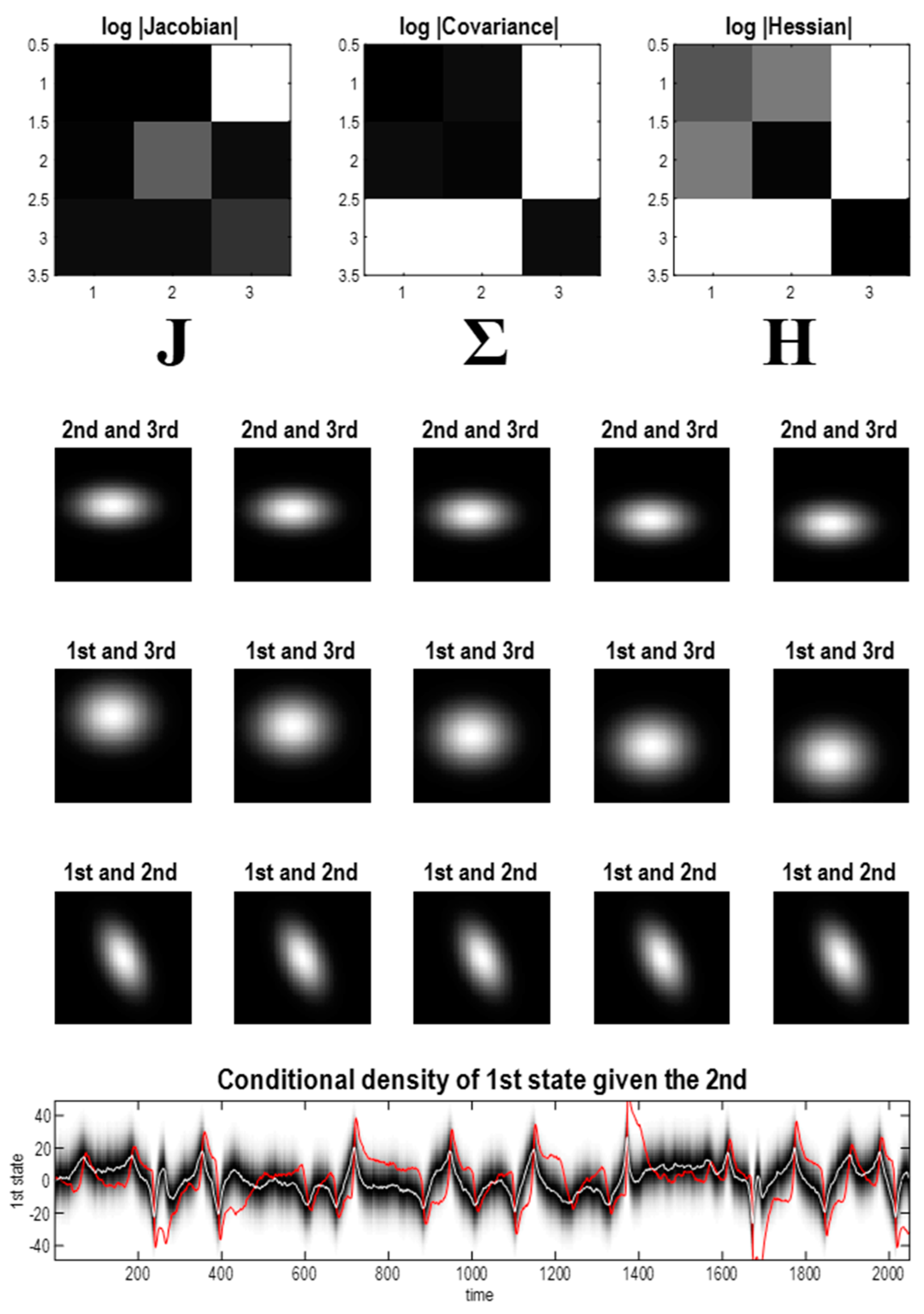
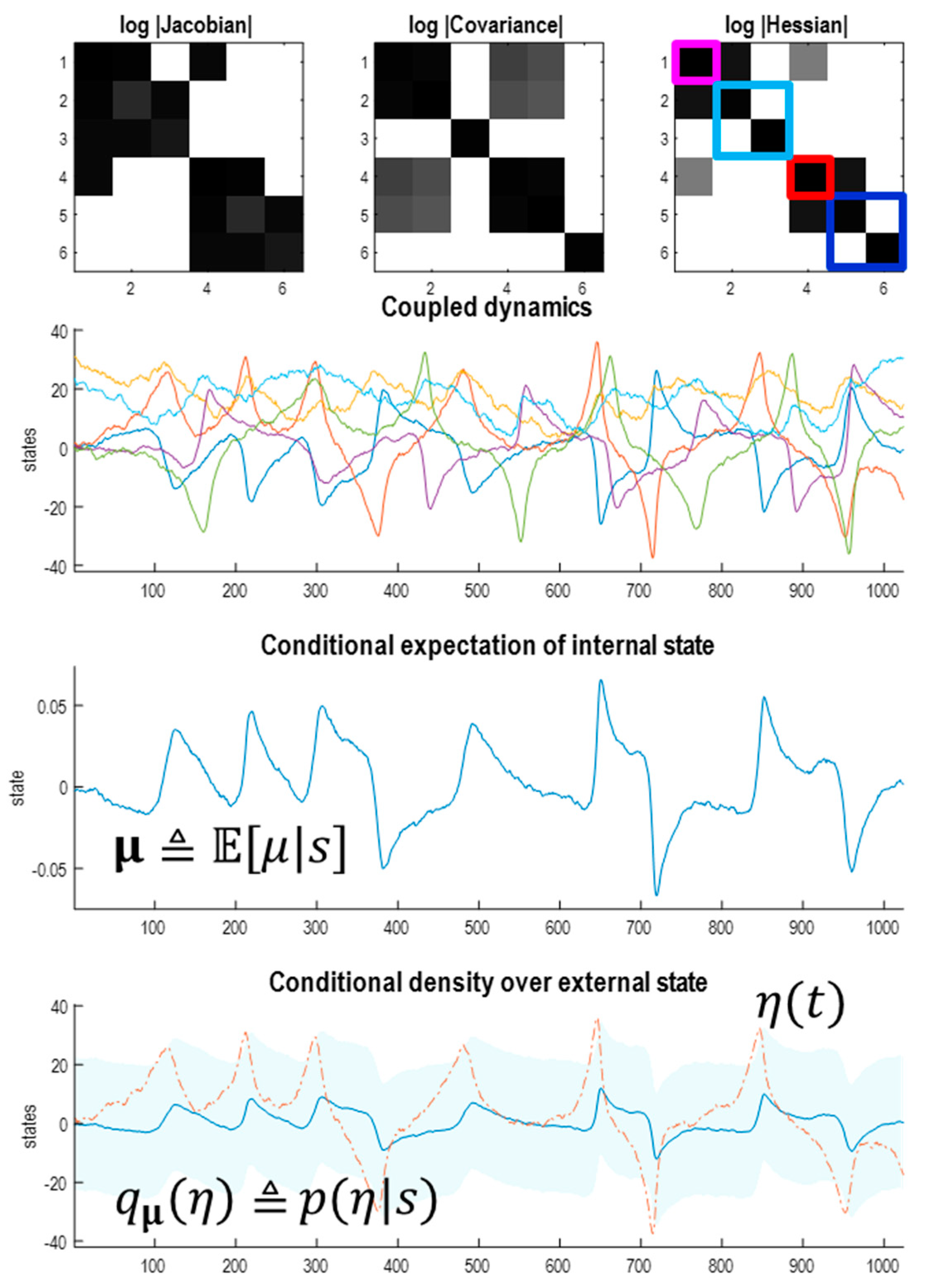
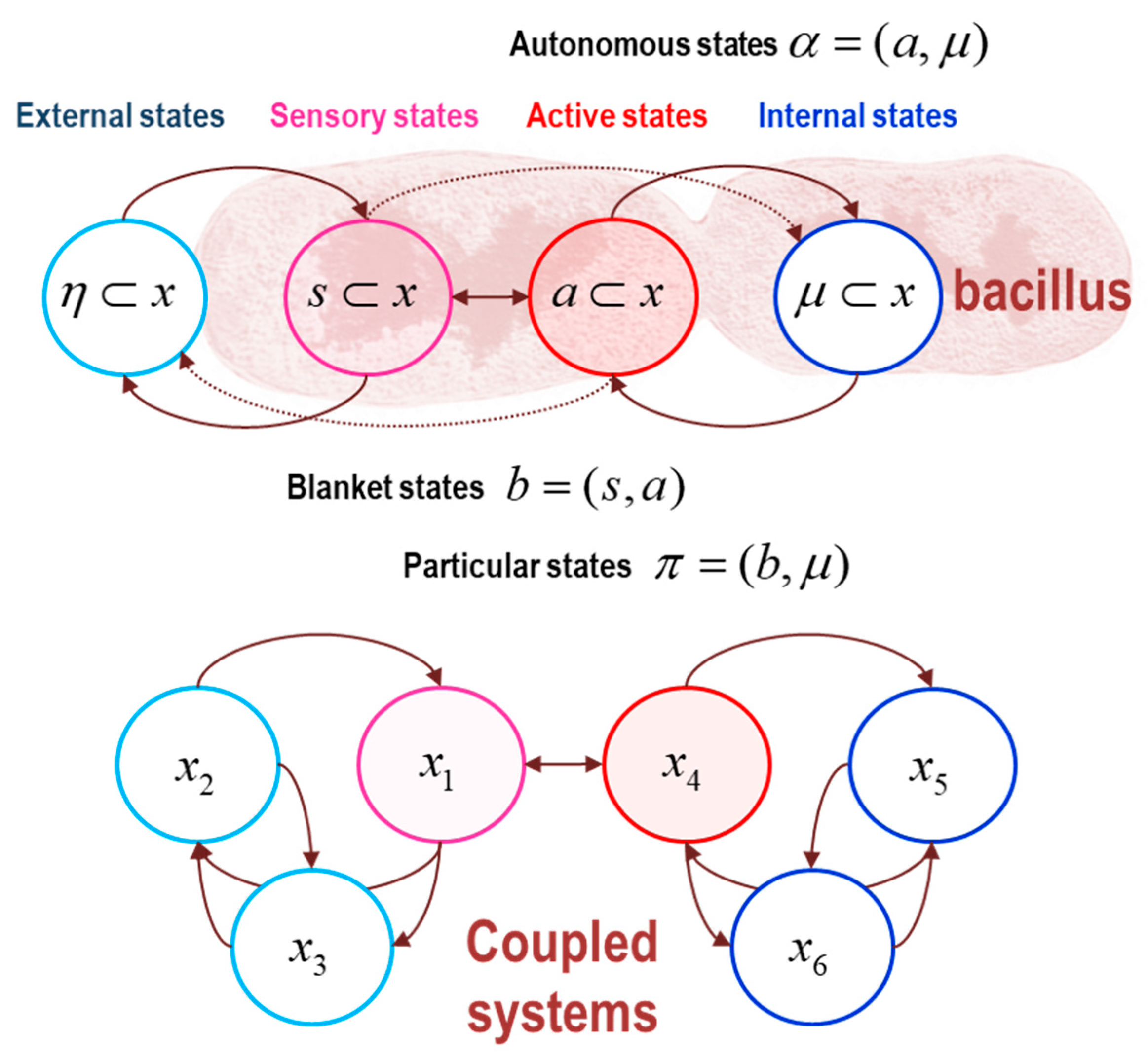
- The Markov boundary of a set of internal states is the minimal set of states for which there exists a nonzero Hessian submatrix:. In other words, the internal states are independent of the remaining states, when conditioned upon their Markov boundary, which we will call active states. The combination of active and internal states will be referred to as autonomous states: ;
- The Markov boundary of autonomous states is the minimal set of states for which there exists a nonzero Hessian submatrix:. In other words, the autonomous states are independent of the remaining states, when conditioned upon their Markov boundary, which we will call sensory states. The combination of sensory and autonomous states will be referred to as particular states: .The combination of active and sensory (i.e., boundary) states constitute blanket states: ;
- The remaining states constitute external states: .
- The minimal set of states for which there exists a nonzero Hessian submatrix: contains the first state, which we designate as the sensory state;
- The particular states now comprise the autonomous states and the first state of the first Lorenz system. The blanket states therefore comprise the first states of each system;
- The remaining external states comprise the last pair of states of the first Lorenz system. The ensuing particular partition is shown schematically in the lower panel of Figure 10.
5. The Free Energy Principle
5.1. The Generative Model and Self-Evidencing
5.2. Summary
6. Discussion
Author Contributions
Funding
Data Availability Statement
Conflicts of Interest
Appendix A
Appendix A.1. Exact Laplacian Form of the Lorenz System
Appendix A.2. Information Length
Appendix A.3. Origins of the Housekeeping Term
References
- Kwon, C.; Ao, P. Nonequilibrium steady state of a stochastic system driven by a nonlinear drift force. Phys. Rev. E 2011, 84, 061106. [Google Scholar] [CrossRef] [PubMed] [Green Version]
- Ramaswamy, S. The Mechanics and Statistics of Active Matter. Annu. Rev. Condens. Matter Phys. 2010, 1, 323–345. [Google Scholar] [CrossRef] [Green Version]
- Esposito, M.; Harbola, U.; Mukamel, S. Nonequilibrium fluctuations, fluctuation theorems, and counting statistics in quantum systems. Rev. Mod. Phys. 2009, 81, 1665–1702. [Google Scholar] [CrossRef] [Green Version]
- Tomé, T. Entropy Production in Nonequilibrium Systems Described by a Fokker-Planck Equation. Braz. J. Phys. 2006, 36, 1285–1289. [Google Scholar] [CrossRef] [Green Version]
- Seifert, U. Entropy production along a stochastic trajectory and an integral fluctuation theorem. Phys. Rev. Lett. 2005, 95, 040602. [Google Scholar] [CrossRef] [Green Version]
- Ao, P. Laws in Darwinian evolutionary theory. Phys. Life Rev. 2005, 2, 117–156. [Google Scholar] [CrossRef] [Green Version]
- Ao, P. Potential in stochastic differential equations: Novel construction. J. Phys. A Math. Gen. 2004, 37, L25–L30. [Google Scholar] [CrossRef]
- Vespignani, A.; Zapperi, S. How self-organized criticality works: A unified mean-field picture. Phys. Rev. E 1998, 57, 6345–6362. [Google Scholar] [CrossRef] [Green Version]
- Jarzynski, C. Nonequilibrium Equality for Free Energy Differences. Phys. Rev. Lett. 1997, 78, 2690–2693. [Google Scholar] [CrossRef] [Green Version]
- Prigogine, I. Time, Structure, and Fluctuations. Science 1978, 201, 777–785. [Google Scholar] [CrossRef] [Green Version]
- England, J.L. Dissipative adaptation in driven self-assembly. Nat. Nanotechnol. 2015, 10, 919–923. [Google Scholar] [CrossRef]
- England, J.L. Statistical physics of self-replication. J. Chem. Phys. 2013, 139, 121923. [Google Scholar] [CrossRef] [Green Version]
- Friston, K. Life as we know it. J. R. Soc. Interface 2013, 10, 20130475. [Google Scholar] [CrossRef] [Green Version]
- Friston, K.; Ao, P. Free energy, value, and attractors. Comput. Math. Methods Med. 2012, 2012, 937860. [Google Scholar] [CrossRef]
- Friston, K. A free energy principle for a particular physics. arXiv 2019, arXiv:1906.10184. [Google Scholar]
- Da Costa, L.; Friston, K.; Heins, C.; Pavliotis, G.A. Bayesian Mechanics for Stationary Processes. arXiv 2021, arXiv:2106.13830. [Google Scholar]
- Kuznetsov, N.V.; Mokaev, T.N.; Kuznetsova, O.A.; Kudryashova, E.V. The Lorenz system: Hidden boundary of practical stability and the Lyapunov dimension. Nonlinear Dyn. 2020, 102, 713–732. [Google Scholar] [CrossRef]
- Lorenz, E.N. Deterministic nonperiodic flow. J. Atmos. Sci. 1963, 20, 130–141. [Google Scholar] [CrossRef] [Green Version]
- Crauel, H. Global random attractors are uniquely determined by attracting deterministic compact sets. Ann. Mat. Pura Appl. 1999, 4, 57–72. [Google Scholar] [CrossRef]
- Crauel, H.; Flandoli, F. Attractors for Random Dynamical-Systems. Probab. Theory Rel. 1994, 100, 365–393. [Google Scholar] [CrossRef]
- Drótos, G.; Bódai, T.; Tél, T. Probabilistic Concepts in a Changing Climate: A Snapshot Attractor Picture. J. Clim. 2015, 28, 3275–3288. [Google Scholar] [CrossRef]
- Zhang, F.; Xu, L.; Zhang, K.; Wang, E.; Wang, J. The potential and flux landscape theory of evolution. J. Chem. Phys. 2012, 137, 065102. [Google Scholar] [CrossRef]
- Seifert, U. Stochastic thermodynamics, fluctuation theorems and molecular machines. Rep. Prog. Phys. 2012, 75, 126001. [Google Scholar] [CrossRef] [Green Version]
- Ma, Y.; Tan, Q.; Yuan, R.; Yuan, B.; Ao, P. Potential Function in a Continuous Dissipative Chaotic System: Decomposition Scheme and Role of Strange Attractor. Int. J. Bifurc. Chaos 2014, 24, 1450015. [Google Scholar] [CrossRef] [Green Version]
- Arnold, L. Random Dynamical Systems, 1st ed.; Springer: Berlin/Heidelberg, Germany, 1998. [Google Scholar]
- Shi, J.; Chen, T.; Yuan, R.; Yuan, B.; Ao, P. Relation of a new interpretation of stochastic differential equations to Ito process. J. Stat. Phys. 2012, 148, 579–590. [Google Scholar] [CrossRef]
- Ma, Y.-A.; Chen, T.; Fox, E.B. A Complete Recipe for Stochastic Gradient MCMC. arXiv 2015, arXiv:1506.04696. [Google Scholar]
- Ao, P. Emerging of Stochastic Dynamical Equalities and Steady State Thermodynamics from Darwinian Dynamics. Commun. Theor. Phys. 2008, 49, 1073–1090. [Google Scholar] [CrossRef] [PubMed] [Green Version]
- Pavliotis, G.A. Stochastic Processes and Applications: Diffusions Processes, the Fokker-Planck and Langevin Equations; Springer: New York, NY, USA, 2014. [Google Scholar]
- Winn, J.; Bishop, C.M. Variational message passing. J. Mach. Learn. Res. 2005, 6, 661–694. [Google Scholar]
- MacKay, D.J. Free-energy minimisation algorithm for decoding and cryptoanalysis. Electron. Lett. 1995, 31, 445–447. [Google Scholar] [CrossRef]
- Hinton, G.E.; Zemel, R.S. Autoencoders, minimum description length and Helmholtz free energy. In Proceedings of the 6th International Conference on Neural Information Processing Systems, Denver, CO, USA, 29 November–2 December 1993; pp. 3–10. [Google Scholar]
- Palacios, E.R.; Razi, A.; Parr, T.; Kirchhoff, M.; Friston, K. Biological Self-organisation and Markov blankets. bioRxiv 2017. [Google Scholar] [CrossRef] [Green Version]
- Hohwy, J. The Self-Evidencing Brain. Noûs 2016, 50, 259–285. [Google Scholar] [CrossRef]
- Risken, H. Fokker-planck equation. In The Fokker-Planck Equation; Springer: Berlin/Heidelberg, Germany, 1996; pp. 63–95. [Google Scholar]
- Pavlos, G.P.; Karakatsanis, L.P.; Xenakis, M.N. Tsallis non-extensive statistics, intermittent turbulence, SOC and chaos in the solar plasma, Part one: Sunspot dynamics. Phys. A Stat. Mech. Its Appl. 2012, 391, 6287–6319. [Google Scholar] [CrossRef] [Green Version]
- Hunt, B.; Ott, E.; Yorke, J. Differentiable synchronisation of chaos. Phys. Rev. E 1997, 55, 4029–4034. [Google Scholar] [CrossRef] [Green Version]
- Saltzman, B. Finite Amplitude Free Convection as an Initial Value Problem—I. J. Atmos. Sci. 1962, 19, 329–341. [Google Scholar] [CrossRef] [Green Version]
- Agarwal, S.; Wettlaufer, J.S. Maximal stochastic transport in the Lorenz equations. Phys. Lett. A 2016, 380, 142–146. [Google Scholar] [CrossRef] [Green Version]
- Poland, D. Cooperative catalysis and chemical chaos: A chemical model for the Lorenz equations. Phys. D 1993, 65, 86–99. [Google Scholar] [CrossRef]
- Barp, A.; Takao, S.; Betancourt, M.; Arnaudon, A.; Girolami, M. A Unifying and Canonical Description of Measure-Preserving Diffusions. arXiv 2021, arXiv:2105.02845. [Google Scholar]
- Eyink, G.L.; Lebowitz, J.L.; Spohn, H. Hydrodynamics and fluctuations outside of local equilibrium: Driven diffusive systems. J. Stat. Phys. 1996, 83, 385–472. [Google Scholar] [CrossRef]
- Graham, R. Covariant formulation of non-equilibrium statistical thermodynamics. Z. Phys. B Condens. Matter 1977, 26, 397–405. [Google Scholar] [CrossRef]
- Amari, S.-I. Natural Gradient Works Efficiently in Learning. Neural Comput. 1998, 10, 251–276. [Google Scholar] [CrossRef]
- Girolami, M.; Calderhead, B. Riemann manifold Langevin and Hamiltonian Monte Carlo methods. J. R. Stat. Soc. Ser. B (Stat. Methodol.) 2011, 73, 123–214. [Google Scholar] [CrossRef]
- Yuan, R.; Ma, Y.; Yuan, B.; Ao, P. Potential function in dynamical systems and the relation with Lyapunov function. In Proceedings of the 30th Chinese Control Conference, Yantai, China, 22–24 July 2011; pp. 6573–6580. [Google Scholar]
- Friston, K.; Mattout, J.; Trujillo-Barreto, N.; Ashburner, J.; Penny, W. Variational free energy and the Laplace approximation. NeuroImage 2007, 34, 220–234. [Google Scholar] [CrossRef]
- Cornish, N.J.; Littenberg, T.B. Tests of Bayesian model selection techniques for gravitational wave astronomy. Phys. Rev. D 2007, 76, 083006. [Google Scholar] [CrossRef] [Green Version]
- Kaplan, J.; Yorke, J. Chaotic behavior of multidimensional difference equations. In Functional Differential Equations and Approximation of Fixed Points; Springer: Berlin/Heidelberg, Germany, 1979. [Google Scholar]
- Leonov, G.A.; Kuznetsov, N.V.; Korzhemanova, N.A.; Kusakin, D.V. Lyapunov dimension formula for the global attractor of the Lorenz system. Commun. Nonlinear Sci. Numer. Simul. 2016, 41, 84–103. [Google Scholar] [CrossRef] [Green Version]
- Baba, K.; Shibata, R.; Sibuya, M. Partial correlation and conditional correlation as measures of conditional independence. Aust. N. Z. J. Stat. 2004, 46, 657–664. [Google Scholar] [CrossRef]
- Kim, E.-J. Investigating Information Geometry in Classical and Quantum Systems through Information Length. Entropy 2018, 20, 574. [Google Scholar] [CrossRef] [PubMed] [Green Version]
- Crooks, G.E. Measuring thermodynamic length. Phys. Rev. Lett. 2007, 99, 100602. [Google Scholar] [CrossRef] [PubMed] [Green Version]
- Caticha, A. Entropic Dynamics. Entropy 2015, 17, 6110. [Google Scholar] [CrossRef] [Green Version]
- Caticha, A. The Basics of Information Geometry. Aip Conf. Proc. 2015, 1641, 15–26. [Google Scholar]
- Barreto, E.; Josic, K.; Morales, C.J.; Sander, E.; So, P. The geometry of chaos synchronization. Chaos 2003, 13, 151–164. [Google Scholar] [CrossRef] [PubMed]
- Rulkov, N.F.; Sushchik, M.M.; Tsimring, L.S.; Abarbanel, H.D. Generalized synchronization of chaos in directionally coupled chaotic systems. Phys. Rev. E Stat. Phys. Plasmas Fluids Relat. Interdiscip. Top. 1995, 51, 980–994. [Google Scholar] [CrossRef] [PubMed]
- Biehl, M.; Pollock, F.A.; Kanai, R. A Technical Critique of Some Parts of the Free Energy Principle. Entropy 2021, 23, 293. [Google Scholar] [CrossRef] [PubMed]
- Friston, K.J.; Da Costa, L.; Parr, T. Some Interesting Observations on the Free Energy Principle. Entropy 2021, 23, 1076. [Google Scholar] [CrossRef] [PubMed]
- Parr, T.; Da Costa, L.; Friston, K. Markov blankets, information geometry and stochastic thermodynamics. Philos. Trans. R. Soc. A Math. Phys. Eng. Sci. 2020, 378, 20190159. [Google Scholar] [CrossRef] [Green Version]
- Beal, M.J. Variational Algorithms for Approximate Bayesian Inference; University of London: London, UK, 2003. [Google Scholar]
- Cannon, W.B. Organization For Physiological Homeostasis. Physiol. Rev. 1929, 9, 399–431. [Google Scholar] [CrossRef]
- Friston, K.J.; Daunizeau, J.; Kilner, J.; Kiebel, S.J. Action and behavior: A free-energy formulation. Biol. Cybern. 2010, 102, 227–260. [Google Scholar] [CrossRef] [Green Version]
- Zeki, S. The Ferrier Lecture 1995 behind the seen: The functional specialization of the brain in space and time. Philos. Trans. R. Soc. Lond. B. Biol. Sci. 2005, 360, 1145–1183. [Google Scholar] [CrossRef] [Green Version]
- Boccaletti, S.; Kurths, J.; Osipov, G.; Valladares, D.L.; Zhou, C.S. The synchronization of chaotic systems. Phys. Rep.-Rev. Sect. Phys. Lett. 2002, 366, 1–101. [Google Scholar] [CrossRef]
- Yildiz, I.B.; von Kriegstein, K.; Kiebel, S.J. From birdsong to human speech recognition: Bayesian inference on a hierarchy of nonlinear dynamical systems. PLoS Comput. Biol. 2013, 9, e1003219. [Google Scholar] [CrossRef]
- Kiebel, S.J.; von Kriegstein, K.; Daunizeau, J.; Friston, K.J. Recognizing sequences of sequences. PLoS Comput. Biol. 2009, 5, e1000464. [Google Scholar] [CrossRef]
- Kiebel, S.J.; Daunizeau, J.; Friston, K.J. Perception and hierarchical dynamics. Front. Neuroinform. 2009, 3, 20. [Google Scholar] [CrossRef] [PubMed] [Green Version]
- Friston, K.; Frith, C. A Duet for one. Conscious. Cogn. 2015, 36, 390–405. [Google Scholar] [CrossRef] [PubMed] [Green Version]
- Friston, K.J.; Frith, C.D. Active inference, communication and hermeneutics. Cortex A J. Devoted Study Nerv. Syst. Behav. 2015, 68, 129–143. [Google Scholar] [CrossRef] [Green Version]
- Isomura, T.; Parr, T.; Friston, K. Bayesian Filtering with Multiple Internal Models: Toward a Theory of Social Intelligence. Neural Comput. 2019, 31, 2390–2431. [Google Scholar] [CrossRef]
- Chen, S.; Billings, S.A.; Grant, P.M. Non-linear system identification using neural networks. Int. J. Control 1990, 51, 1191–1214. [Google Scholar] [CrossRef]
- Paduart, J.; Lauwers, L.; Swevers, J.; Smolders, K.; Schoukens, J.; Pintelon, R. Identification of nonlinear systems using Polynomial Nonlinear State Space models. Automatica 2010, 46, 647–656. [Google Scholar] [CrossRef]
- Pathak, J.; Lu, Z.; Hunt, B.R.; Girvan, M.; Ott, E. Using machine learning to replicate chaotic attractors and calculate Lyapunov exponents from data. Chaos Interdiscip. J. Nonlinear Sci. 2017, 27, 121102. [Google Scholar] [CrossRef]
- Rapaic, M.R.; Kanovic, Z.; Jelicic, Z.D.; Petrovacki, D. Generalized PSO algorithm—An application to Lorenz system identification by means of neural-networks. In Proceedings of the 2008 9th Symposium on Neural Network Applications in Electrical Engineering, Belgrade, Serbia, 25–27 September 2008; pp. 31–35. [Google Scholar]
- Goodfellow, I.; Bengio, Y.; Courville, A. Deep Learning; The MIT Press: Cambridge, MA, USA, 2016. [Google Scholar]
- Hinton, G.E.; Salakhutdinov, R.R. Reducing the Dimensionality of Data with Neural Networks. Science 2006, 313, 504. [Google Scholar] [CrossRef] [Green Version]
- LeCun, Y. Learning Invariant Feature Hierarchies. In Computer Vision–ECCV 2012. Workshops and Demonstrations; Fusiello, A., Murino, V., Cucchiara, R., Eds.; Springer: Berlin\Heidelberg, Germany, 2012; pp. 496–505. [Google Scholar]
- LeCun, Y.; Bengio, Y.; Hinton, G. Deep learning. Nature 2015, 521, 436–444. [Google Scholar] [CrossRef]
- Wang, Y.; Yao, S. Neural Stochastic Differential Equations with Neural Processes Family Members for Uncertainty Estimation in Deep Learning. Sensors 2021, 21, 3708. [Google Scholar] [CrossRef]
- Bejan, A.; Lorente, S. Constructal law of design and evolution: Physics, biology, technology, and society. J. Appl. Phys. 2013, 113, 151301. [Google Scholar] [CrossRef] [Green Version]
- Horowitz, J.M. Multipartite information flow for multiple Maxwell demons. J. Stat. Mech. Theory Exp. 2015, 2015, P03006. [Google Scholar] [CrossRef]
- Haussmann, U.G.; Pardoux, E. Time Reversal of Diffusions. Ann. Probab. 1986, 14, 1188–1205. [Google Scholar] [CrossRef]
- Qian, H. A decomposition of irreversible diffusion processes without detailed balance. J. Math. Phys. 2013, 54, 053302. [Google Scholar] [CrossRef]
- Stackexchange. Available online: https://math.stackexchange.com/questions/78818/what-is-the-divergence-of-a-matrix-valued-function (accessed on 3 July 2021).
- Deen, W.M. Introduction to Chemical Engineering Fluid Mechanics; Cambridge University Press: Cambridge, UK, 2016. [Google Scholar]
- Noferesti, S.; Ghassemi, H.; Nowruzi, H. Numerical investigation on the effects of obstruction and side ratio on non-Newtonian fluid flow behavior around a rectangular barrier. J. Appl. Math. Comput. Mech. 2019, 18, 53–67. [Google Scholar] [CrossRef]


Publisher’s Note: MDPI stays neutral with regard to jurisdictional claims in published maps and institutional affiliations. |
© 2021 by the authors. Licensee MDPI, Basel, Switzerland. This article is an open access article distributed under the terms and conditions of the Creative Commons Attribution (CC BY) license (https://creativecommons.org/licenses/by/4.0/).
Share and Cite
Friston, K.; Heins, C.; Ueltzhöffer, K.; Da Costa, L.; Parr, T. Stochastic Chaos and Markov Blankets. Entropy 2021, 23, 1220. https://doi.org/10.3390/e23091220
Friston K, Heins C, Ueltzhöffer K, Da Costa L, Parr T. Stochastic Chaos and Markov Blankets. Entropy. 2021; 23(9):1220. https://doi.org/10.3390/e23091220
Chicago/Turabian StyleFriston, Karl, Conor Heins, Kai Ueltzhöffer, Lancelot Da Costa, and Thomas Parr. 2021. "Stochastic Chaos and Markov Blankets" Entropy 23, no. 9: 1220. https://doi.org/10.3390/e23091220