
A Thermodynamic Approach to Measuring Entropy in a Few-Electron Nanodevice


Abstract
:1. Introduction
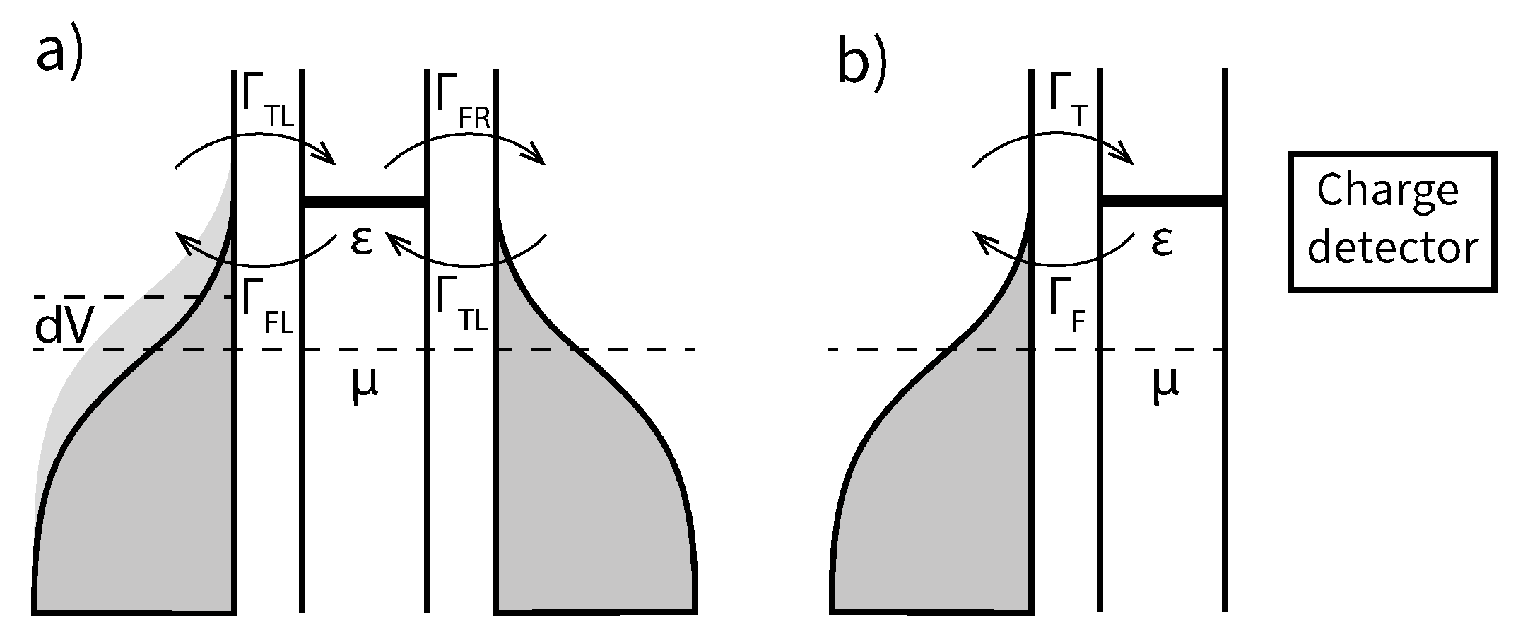
2. The System
3. Rate Equations
3.1. Degeneracy Effects in the Rate Equation
3.2. Detailed Balance Approach to Maxwell Relations
4. Thermodynamic Relation, No Excited States
4.1. Derivation and Entropy Definition
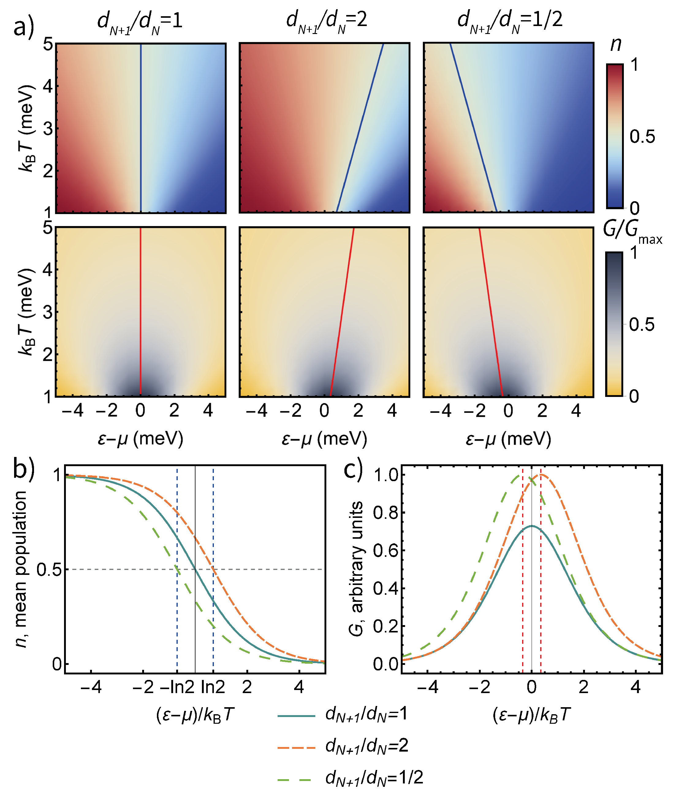
4.2. Applications and Experimental Evidence: A Two-Fold Degenerate Energy Level
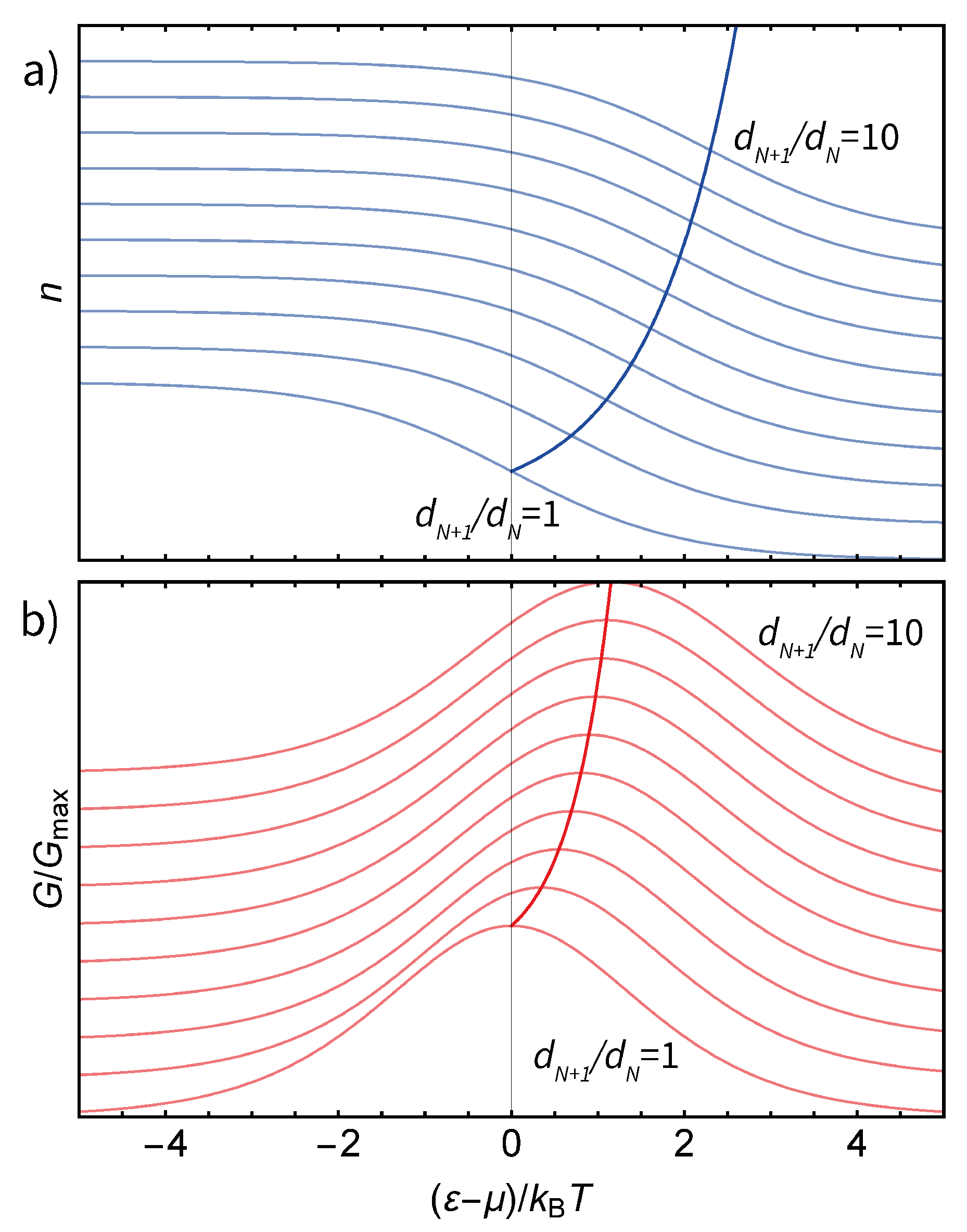
4.3. A Single N-Fold Degenerate Energy Level
5. General Thermodynamic Relation
5.1. Systems with Excited States
5.2. Discussion
6. Conclusions
Author Contributions
Funding
Institutional Review Board Statement
Informed Consent Statement
Data Availability Statement
Acknowledgments
Conflicts of Interest
Appendix A. Proof of Peak Conductance Condition
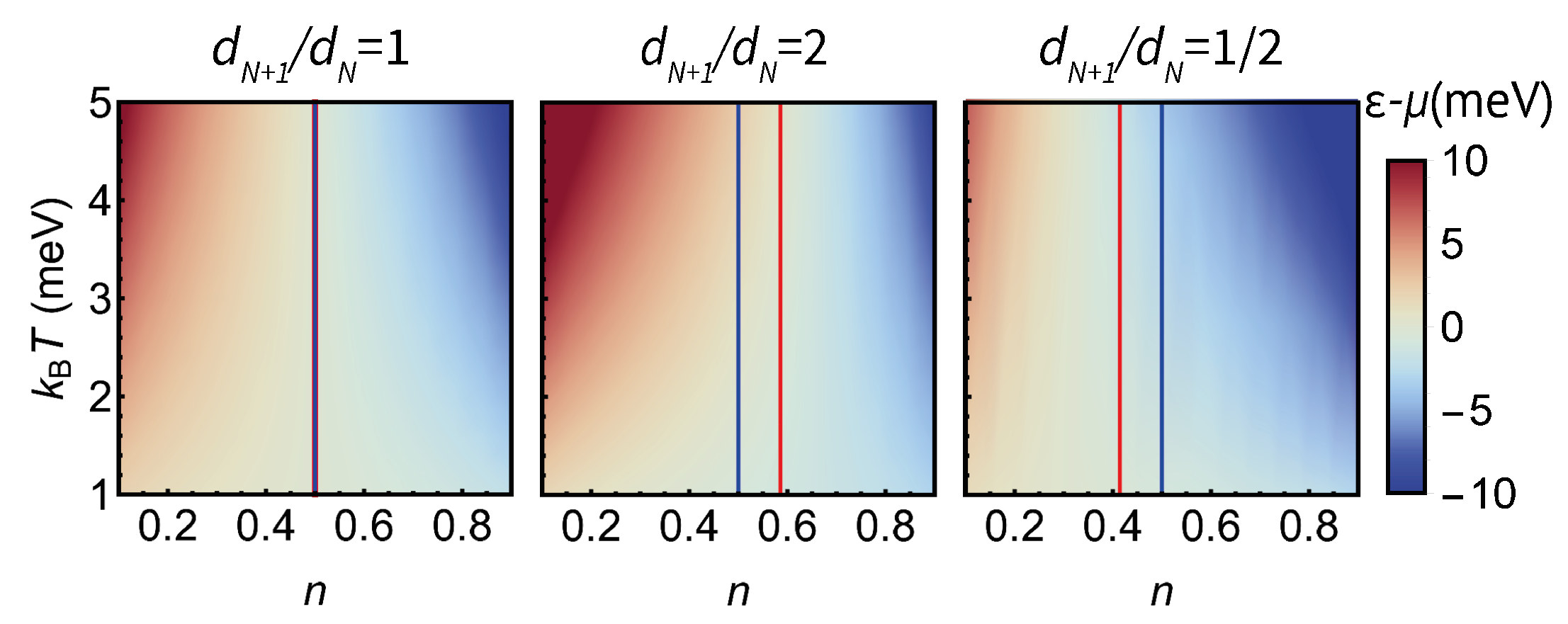
Appendix B. Dot Population from the Maxwell Relation
Appendix C. Independent Proof
References
- Ramirez, A.P.; Hayashi, A.; Cava, R.J.; Siddharthan, R.; Shastry, B.S. Zero-point entropy in ‘spin ice’. Nature 1999, 399, 333–335. [Google Scholar] [CrossRef]
- Gornik, E.; Lassnig, R.; Strasser, G.; Störmer, H.L.; Gossard, A.C.; Wiegmann, W. Specific heat of two-dimensional electrons in GaAs-GaAlAs multilayers. Phys. Rev. Lett. 1985, 54, 1820–1823. [Google Scholar] [CrossRef]
- Wang, J.K.; Campbell, J.H.; Tsui, D.C.; Cho, A.Y. Heat capacity of the two-dimensional electron gas in GaAs/AlxGa1-xAs multiple-quantum-well structures. Phys. Rev. B 1988, 38, 6174–6184. [Google Scholar] [CrossRef]
- Bayot, V.; Grivei, E.; Melinte, S.; Santos, M.B.; Shayegan, M. Giant low temperature heat capacity of GaAs quantum wells near landau level filling ν = 1. Phys. Rev. Lett. 1996, 76, 4584–4587. [Google Scholar] [CrossRef] [Green Version]
- Schulze-Wischeler, F.; Zeitler, U.; Zobeltitz, C.V.; Hohls, F.; Reuter, D.; Wieck, A.D.; Frahm, H.; Haug, R.J. Measurement of the specific heat of a fractional quantum Hall system. Phys. Rev. B-Condens. Matter Mater. Phys. 2007, 76, 4–7. [Google Scholar] [CrossRef]
- Schmidt, B.A.; Bennaceur, K.; Gaucher, S.; Gervais, G.; Pfeiffer, L.N.; West, K.W. Specific heat and entropy of fractional quantum Hall states in the second Landau level. Phys. Rev. B 2017, 95, 1–5. [Google Scholar] [CrossRef] [Green Version]
- Josefsson, M.; Svilans, A.; Burke, A.M.; Hoffmann, E.A.; Fahlvik, S.; Thelander, C.; Leijnse, M.; Linke, H. A quantum-dot heat engine operating close to the thermodynamic efficiency limits. Nat. Nanotechnol. 2018, 13, 920–924. [Google Scholar] [CrossRef] [Green Version]
- Harzheim, A.; Sowa, J.K.; Swett, J.L.; Briggs, G.A.D.; Mol, J.A.; Gehring, P. Role of metallic leads and electronic degeneracies in thermoelectric power generation in quantum dots. Phys. Rev. Res. 2020, 2, 013140. [Google Scholar] [CrossRef] [Green Version]
- Reddy, P.; Jang, S.Y.; Segalman, R.A.; Majumdar, A. Thermoelectricity in Molecular Junctions. Science 2007, 315, 1568–1571. [Google Scholar] [CrossRef] [PubMed]
- Zotti, L.A.; Bürkle, M.; Pauly, F.; Lee, W.; Kim, K.; Jeong, W.; Asai, Y.; Reddy, P.; Cuevas, J.C. Heat dissipation and its relation to thermopower in single-molecule junctions. New J. Phys. 2014, 16. [Google Scholar] [CrossRef]
- Cui, L.; Miao, R.; Wang, K.; Thompson, D.; Zotti, L.A.; Cuevas, J.C.; Meyhofer, E.; Reddy, P. Peltier cooling in molecular junctions. Nat. Nanotechnol. 2018, 13, 122–127. [Google Scholar] [CrossRef] [PubMed]
- Rossnagel, J.; Dawkins, S.T.; Tolazzi, K.N.; Abah, O.; Lutz, E.; Schmidt-Kaler, F.; Singer, K. A single-atom heat engine. Science 2016, 352, 325–329. [Google Scholar] [CrossRef] [Green Version]
- Lutz, E. A single-atom heat engine. Phys. Today 2020, 73, 66–67. [Google Scholar] [CrossRef]
- Micadei, K.; Peterson, J.P.S.; Souza, A.M.; Sarthour, R.S.; Oliveira, I.S.; Landi, G.T.; Batalhão, T.B.; Serra, R.M.; Lutz, E. Reversing the direction of heat flow using quantum correlations. Nat. Commun. 2019, 10, 2456. [Google Scholar] [CrossRef]
- Hartman, N.; Olsen, C.; Lüscher, S.; Samani, M.; Fallahi, S.; Gardner, G.C.; Manfra, M.; Folk, J. Direct entropy measurement in a mesoscopic quantum system. Nat. Phys. 2018, 14, 1083–1086. [Google Scholar] [CrossRef]
- Sela, E.; Oreg, Y.; Plugge, S.; Hartman, N.; Lüscher, S.; Folk, J. Detecting the Universal Fractional Entropy of Majorana Zero Modes. Phys. Rev. Lett. 2019, 123, 147702. [Google Scholar] [CrossRef] [PubMed] [Green Version]
- Kleeorin, Y.; Thierschmann, H.; Buhmann, H.; Georges, A.; Molenkamp, L.W.; Meir, Y. How to measure the entropy of a mesoscopic system via thermoelectric transport. Nat. Commun. 2019, 10, 1–8. [Google Scholar] [CrossRef]
- Gehring, P.; Sowa, J.K.; Hsu, C.; de Bruijckere, J.; van der Star, M.; Le Roy, J.J.; Bogani, L.; Gauger, E.M.; van der Zant, H.S.J. Complete mapping of the thermoelectric properties of a single molecule. Nat. Nanotechnol. 2021, 1–26. [Google Scholar] [CrossRef]
- Brooke, C.; Vezzoli, A.; Higgins, S.J.; Zotti, L.A.; Palacios, J.J.; Nichols, R.J. Resonant transport and electrostatic effects in single-molecule electrical junctions. Phys. Rev. B-Condens. Matter Mater. Phys. 2015, 91, 1–9. [Google Scholar] [CrossRef] [Green Version]
- Nazarov, Y.V.; Blanter, Y.M. Quantum Transport; Cambridge University Press: Cambridge, UK, 2009. [Google Scholar] [CrossRef]
- Hanson, R.; Kouwenhoven, L.P.; Petta, J.R.; Tarucha, S.; Vandersypen, L.M. Spins in few-electron quantum dots. Rev. Mod. Phys. 2007, 79, 1217–1265. [Google Scholar] [CrossRef] [Green Version]
- Beckel, A.; Kurzmann, A.; Geller, M.; Ludwig, A.; Wieck, A.D.; König, J.; Lorke, A. Asymmetry of charge relaxation times in quantum dots: The influence of degeneracy. Epl 2014, 106. [Google Scholar] [CrossRef] [Green Version]
- Hofmann, A.; Maisi, V.F.; Gold, C.; Krähenmann, T.; Rössler, C.; Basset, J.; Märki, P.; Reichl, C.; Wegscheider, W.; Ensslin, K.; et al. Measuring the degeneracy of discrete energy levels using a GaAs/AlGaAs quantum dot. Phys. Rev. Lett. 2016, 117, 1–6. [Google Scholar] [CrossRef] [Green Version]
- Beenakker, C.W.J. Theory of Coulomb-blockade oscillations in the conductance of a quantum dot. Phys. Rev. B 1991, 44, 1646–1656. [Google Scholar] [CrossRef] [PubMed] [Green Version]
- Cooper, N.R.; Stern, A. Observable bulk signatures of Nnon-Abelian quantum hall states. Phys. Rev. Lett. 2009, 102, 1–4. [Google Scholar] [CrossRef] [PubMed] [Green Version]
- Ben-Shach, G.; Laumann, C.R.; Neder, I.; Yacoby, A.; Halperin, B.I. Detecting non-abelian anyons by charging spectroscopy. Phys. Rev. Lett. 2013, 110, 1–5. [Google Scholar] [CrossRef] [Green Version]
- Kim, Y.; Jeong, W.; Kim, K.; Lee, W.; Reddy, P. Electrostatic control of thermoelectricity in molecular junctions. Nat. Nanotechnol. 2014, 9, 881–885. [Google Scholar] [CrossRef]
- Sowa, J.K.; Mol, J.A.; Gauger, E.M. Marcus Theory of Thermoelectricity in Molecular Junctions. J. Phys. Chem. C 2019, 123, 4103–4108. [Google Scholar] [CrossRef]
- Sowa, J.K.; Mol, J.A.; Briggs, G.A.D.; Gauger, E.M. Beyond Marcus theory and the Landauer-Büttiker approach in molecular junctions: A unified framework. J. Chem. Phys. 2018, 149. [Google Scholar] [CrossRef]


Publisher’s Note: MDPI stays neutral with regard to jurisdictional claims in published maps and institutional affiliations. |
© 2021 by the authors. Licensee MDPI, Basel, Switzerland. This article is an open access article distributed under the terms and conditions of the Creative Commons Attribution (CC BY) license (https://creativecommons.org/licenses/by/4.0/).
Share and Cite
Pyurbeeva, E.; Mol, J.A. A Thermodynamic Approach to Measuring Entropy in a Few-Electron Nanodevice. Entropy 2021, 23, 640. https://doi.org/10.3390/e23060640
Pyurbeeva E, Mol JA. A Thermodynamic Approach to Measuring Entropy in a Few-Electron Nanodevice. Entropy. 2021; 23(6):640. https://doi.org/10.3390/e23060640
Chicago/Turabian StylePyurbeeva, Eugenia, and Jan A. Mol. 2021. "A Thermodynamic Approach to Measuring Entropy in a Few-Electron Nanodevice" Entropy 23, no. 6: 640. https://doi.org/10.3390/e23060640