Natural Time Analysis of Seismicity within the Mexican Flat Slab before the M7.1 Earthquake on 19 September 2017

 ,
,  , and
, and 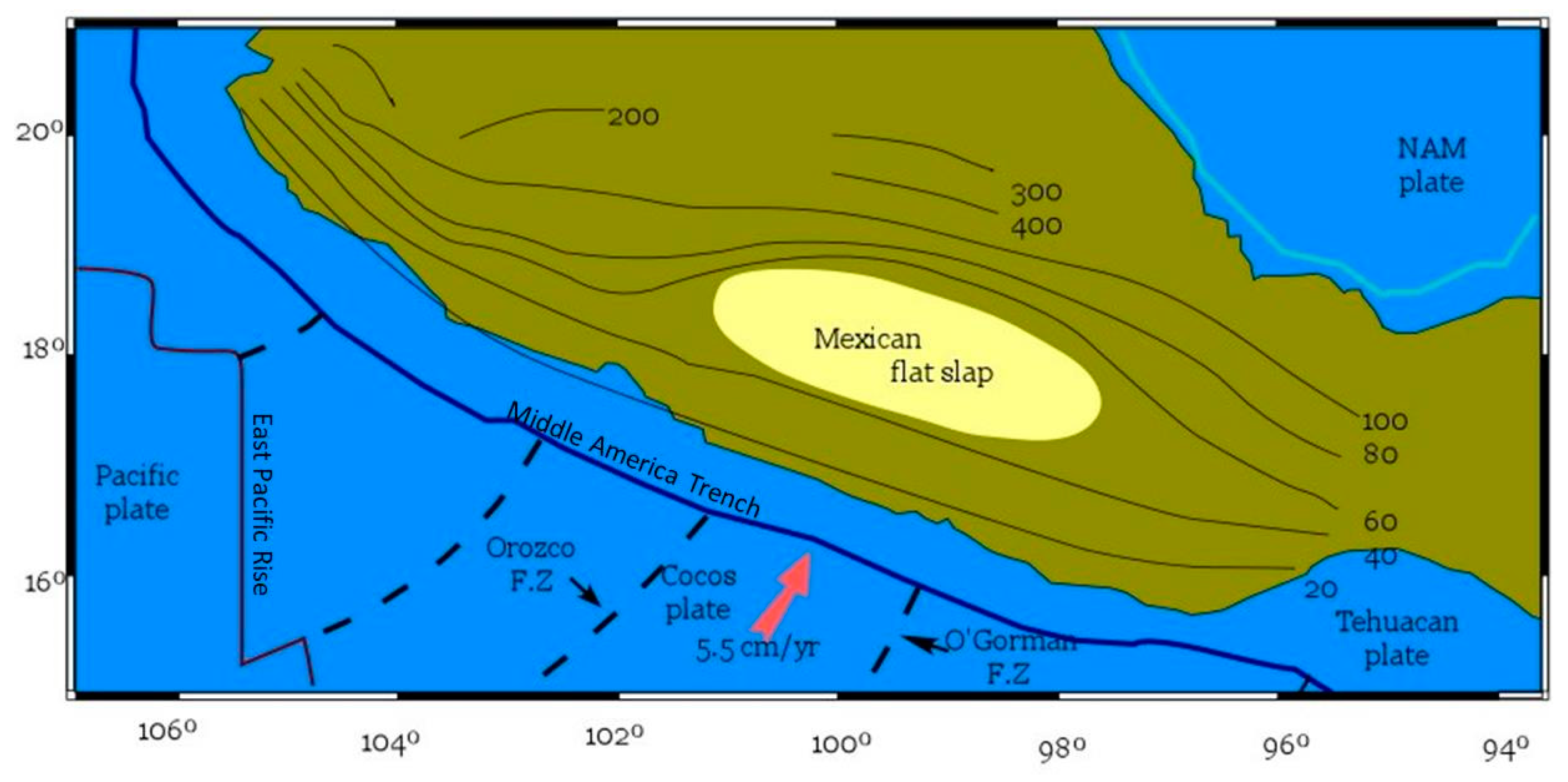
Abstract
:1. Introduction
2. Methodology
2.1. Natural Time Analysis
2.2. Nowcasting
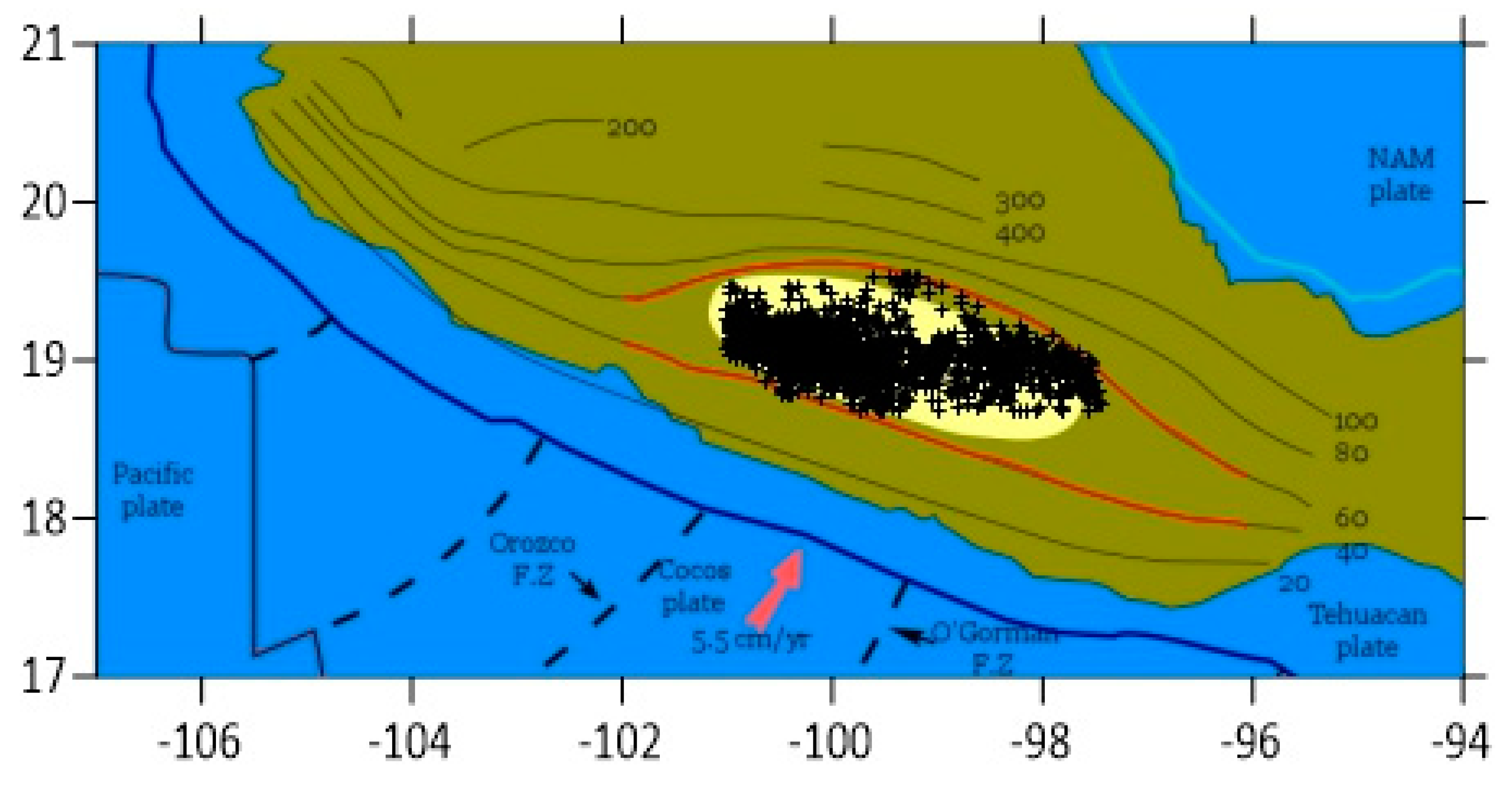
3. Tectonic Subduction Structure
4. Data and Analysis
5. Results
5.1. Entropy in Natural Time Domain
5.2. Variability Analysis
5.3. Identifying the Time of the Impending Mainshock
- (i)
- The “average” distance between the curves of of the evolving seismicity and Equation (6) should be < 10−2.
- (ii)
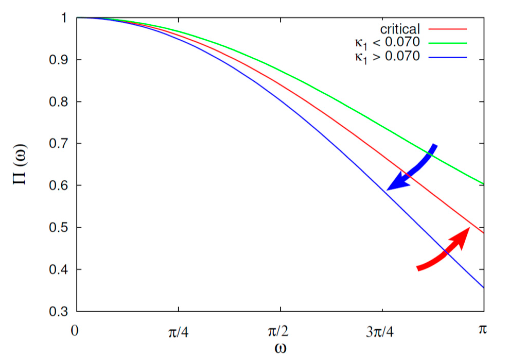
- The final approach of the evolving to that of Equation (6) must be from below as shown by the red arrow in Figure 5 (while the blue arrow indicates the opposite behavior). This reflects that gradually changes with time before strong EQs finally approaching from above that of the critical state, i.e., = 0.070, as depicted by the inset of Figure 5.
- (iii)
- At the coincidence, both entropies S and S_ must be smaller than Su.
- (iv)
- Since this process (critical dynamics) is supposed to be self-similar, the occurrence time of the true coincidence should not vary markedly upon changing the threshold Mthres.
5.4. Nowcasting Analysis
6. Main Conclusions
Author Contributions
Funding
Acknowledgments
Conflicts of Interest
References
- Manea, V.; Manea, M.; Ferrari, L.; Orozco-Esquivel, T.; Valenzuela, R.; Husker, A.; Kostoglodov, V. A review of the geodynamic evolution of flat slab subduction in Mexico, Peru, and Chile. Tectonophysics 2017, 695, 27–52. [Google Scholar] [CrossRef]
- Uyeda, S.; Kanamori, H. Back-arc opening and the mode of subduction. J. Geophys. Res. 1979, 84, 1049–1061. [Google Scholar] [CrossRef] [Green Version]
- Sarlis, N.V.; Skordas, E.S.; Varotsos, P.A.; Ramírez-Rojas, A.; Flores-Márquez, E.L. Natural time analysis: On the deadly Mexico M8.2 earthquake on 7 September 2017. Phys. A 2018, 506, 625–634. [Google Scholar] [CrossRef]
- Ramírez-Rojas, A.; Flores-Márquez, E.L.; Sarlis, N.V.; Varotsos, P.A. The Complexity Measures Associated with the Fluctuations of the Entropy in Natural Time before the Deadly Mexico M8.2 Earthquake on 7 September 2017. Entropy 2018, 20, 477. [Google Scholar] [CrossRef] [Green Version]
- Sarlis, N.V.; Skordas, E.S.; Varotsos, P.A.; Ramírez-Rojas, A.; Flores-Márquez, E.L. Identifying the Occurrence Time of the Deadly Mexico M8.2 Earthquake on 7 September 2017. Entropy 2019, 21, 301. [Google Scholar] [CrossRef] [Green Version]
- Sarlis, N.V.; Skordas, E.S.; Varotsos, P.A.; Ramírez-Rojas, A.; Flores-Márquez, E.L. Investigation of the temporal correlations between earthquake magnitudes before the Mexico M8.2 earthquake on 7 September 2017. Phys. A 2019, 517, 475–483. [Google Scholar] [CrossRef]
- Ramırez-Rojas, A.; Pavıa-Miller, C.G.; Angulo-Brown, F. Statistical behavior of the spectral exponent and the correlation time of electric self-potential time series associated to the Ms = 7.4 September 14, 1995 earthquake in Mexico. Phys. Chem. Earth Parts A/B/C 2004, 29, 305–312. [Google Scholar] [CrossRef]
- Cervantes de la Torre, F.; Ramírez-Rojas, A.; Pavía-Miller, C.G.; Angulo-Brown, F.; Yépez, E.; Peralta, J.A. A comparison between spectral and fractal methods in electrotelluric time series. Rev. Mex. Fis. 1999, 45, 298–302. Available online: https://rmf.smf.mx/ojs/rmf/article/view/2863/2831 (accessed on 8 May 2020).
- Abe, S.; Suzuki, N. Scale-free network of earthquakes. EPL 2004, 65, 581–586. [Google Scholar] [CrossRef] [Green Version]
- Abe, S.; Suzuki, N. Complex-network description of seismicity. Nonlin. Process. Geophys. 2006, 13, 145–150. [Google Scholar] [CrossRef]
- Tenenbaum, J.N.; Havlin, S.; Stanley, H.E. Earthquake networks based on similar activity patterns. Phys. Rev. E 2012, 86, 046107. [Google Scholar] [CrossRef] [PubMed] [Green Version]
- Sarlis, N.V.; Skordas, E.S.; Varotsos, P.A. A remarkable change of the entropy of seismicity in natural time under time reversal before the super-giant M9 Tohoku earthquake on 11 March 2011. EPL 2018, 124, 29001. [Google Scholar] [CrossRef]
- Ohsawa, Y. Regional Seismic Information Entropy to Detect Earthquake Activation Precursors. Entropy 2018, 20, 861. [Google Scholar] [CrossRef] [Green Version]
- Rundle, J.B.; Giguere, A.; Turcotte, D.L.; Crutchfield, J.P.; Donnellan, A. Global Seismic Nowcasting With Shannon Information Entropy. Earth Space Sci. 2019, 6, 191–197. [Google Scholar] [CrossRef] [PubMed] [Green Version]
- Telesca, L.; Lapenna, V.; Macchiato, M. Mono- and multi-fractal investigation of scaling properties in temporal patterns of seismic sequences. Chaos. Soliton Fractals 2004, 19, 1–15. [Google Scholar] [CrossRef]
- Aggarwal, S.K.; Lovallo, M.; Khan, P.K.; Rastogi, B.K.; Telesca, L. Multifractal detrended fluctuation analysis of magnitude series of seismicity of Kachchh region, Western India. Phys. A 2015, 426, 56–62. [Google Scholar] [CrossRef]
- Telesca, L.; Cuomo, V.; Lapenna, V.; Macchiato, M. Statistical analysis of fractal properties of point processes modeling seismic sequences. Phys. Earth Planet. Inter. 2001, 125, 65–83. [Google Scholar] [CrossRef]
- Telesca, L.; Cuomo, V.; Lapenna, V.; Macchiato, M. Depth-dependent time-clustering behaviour in seismicity of southern California. Geophys. Res. Lett. 2001, 28, 4323–4326. [Google Scholar] [CrossRef]
- Cervantes de la Torre, F.; Pavía-Miller, C.; Ramirez-Rojas, A.; Angulo-Brown, F. Time Evolution of the Fractal Dimension of Electric Self-Potential Time Series. Nonlinear Dyn. Geosci. 2007, 407–418. [Google Scholar] [CrossRef]
- Flores-Márquez, L.; Márquez-Cruz, J.; Ramírez-Rojas, A.; Gálvez-Coyt, G.; Angulo-Brown, F. A statistical analysis of electric self-potential time series associated to two 1993 earthquakes in Mexico. Nat. Hazards Earth Syst. Sci. 2007, 7, 549–556. [Google Scholar] [CrossRef]
- Varotsos, P.A.; Sarlis, N.V.; Skordas, E.S. Natural Time Analysis: The New View of Time. Precursory Seismic Electric Signals, Earthquakes and Other Complex; Time-Series; Springer: Berlin/Heidelberg, Germany, 2011. [Google Scholar] [CrossRef]
- Varotsos, P.A.; Sarlis, N.V.; Skordas, E.S. Spatio-Temporal complexity aspects on the interrelation between Seismic Electric Signals and Seismicity. Pract. Athens Acad. 2001, 76, 294–321. Available online: http://physlab.phys.uoa.gr/org/pdf/p3.pdf (accessed on 8 May 2020).
- Varotsos, P.A.; Sarlis, N.V.; Tanaka, H.K.; Skordas, E.S. Similarity of fluctuations in correlated systems: The case of seismicity. Phys. Rev. E 2005, 72, 41103. [Google Scholar] [CrossRef] [Green Version]
- Varotsos, P.A.; Sarlis, N.V.; Tanaka, H.K.; Skordas, E.S. Some properties of the entropy in the natural time. Phys. Rev. E 2005, 71, 32102. [Google Scholar] [CrossRef] [PubMed] [Green Version]
- Varotsos, P.A.; Sarlis, N.V.; Skordas, E.S.; Lazaridou, M.S. Identifying sudden cardiac death risk and specifying its occurrence time by analyzing electrocardiograms in natural time. Appl. Phys. Lett. 2007, 91, 64106. [Google Scholar] [CrossRef]
- Rundle, J.B.; Turcotte, D.L.; Donnellan, A.; Grant Ludwig, L.; Luginbuhl, M.; Gong, G. Nowcasting earthquakes. Earth Space Sci. 2016, 3, 480–486. [Google Scholar] [CrossRef]
- Rundle, J.B.; Luginbuhl, M.; Giguere, A.; Turcotte, D.L. Natural Time, Nowcasting and the Physics of Earthquakes: Estimation of Seismic Risk to Global Megacities. Pure Appl. Geophys. 2018, 175, 647–660. [Google Scholar] [CrossRef] [Green Version]
- Luginbuhl, M.; Rundle, J.B.; Turcotte, D.L. Natural Time and Nowcasting Earthquakes: Are Large Global Earthquakes Temporally Clustered? Pure Appl. Geophys. 2018, 175, 661–670. [Google Scholar] [CrossRef]
- Luginbuhl, M.; Rundle, J.B.; Hawkins, A.; Turcotte, D.L. Nowcasting Earthquakes: A Comparison of Induced Earthquakes in Oklahoma and at the Geysers, California. Pure Appl. Geophys. 2018, 175, 49–65. [Google Scholar] [CrossRef]
- Rundle, J.B.; Luginbuhl, M.; Khapikova, P.; Turcotte, D.L.; Donnellan, A.; McKim, G. Nowcasting Great Global Earthquake and Tsunami Sources. Pure Appl. Geophys. 2020, 177, 359–368. [Google Scholar] [CrossRef]
- Varotsos, P.A.; Sarlis, N.V.; Skordas, E.S. On the Motivation and Foundation of Natural Time Analysis: Useful Remarks. Acta Geophys. 2016, 64, 841–852. [Google Scholar] [CrossRef] [Green Version]
- Sarlis, N.V.; Christopoulos, S.-R.G.; Bemplidaki, M.M. Change ΔS of the entropy in natural time under time reversal: Complexity measures upon change of scale. EPL 2015, 109, 18002. [Google Scholar] [CrossRef] [Green Version]
- Baldoumas, G.; Peschos, D.; Tatsis, G.; Chronopoulos, S.K.; Christofilakis, V.; Kostarakis, P.; Varotsos, P.; Sarlis, N.V.; Skordas, E.S.; Bechlioulis, A.; et al. A Prototype Photoplethysmography Electronic Device that Distinguishes Congestive Heart Failure from Healthy Individuals by Applying Natural Time Analysis. Electronics 2019, 8, 1288. [Google Scholar] [CrossRef] [Green Version]
- Chelidze, T.; Telesca, L.; Vallianatos, F. Complexity of Seismic Time Series: Measurement and Application; Elsevier: Amsterdam, The Netherlands, 2008. [Google Scholar] [CrossRef]
- Vallianatos, F.; Michas, G.; Benson, P.; Sammonds, P. Natural time analysis of critical phenomena: The case of acoustic emissions in triaxially deformed Etna basalt. Phys. A Stat. Mech. Appl. 2013, 20, 5172–5178. [Google Scholar] [CrossRef]
- Vallianatos, F.; Michas, G.; Hloupis, G. Multiresolution wavelets and natural time analysis before the January-February 2014 Cephalonia (Mw6.1 & 6.0) sequence of strong earthquake events. Phys. Chem. Earth 2015, 85–86, 201–209. [Google Scholar] [CrossRef]
- Skordas, E.S.; Christopoulos, S.-R.G.; Sarlis, N.V. Detrended fluctuation analysis of seismicity and order parameter fluctuations before the M7.1 Ridgecrest earthquake. Nat. Hazards 2020, 100, 697–711. [Google Scholar] [CrossRef]
- Christopoulos, S.-R.G.; Skordas, E.S.; Sarlis, N.V. On the Statistical Significance of the Variability Minima of the Order Parameter of Seismicity by Means of Event Coincidence Analysis. Appl. Sci. 2020, 10, 662. [Google Scholar] [CrossRef] [Green Version]
- Varotsos, C.A.; Lovejoy, S.; Sarlis, N.V.; Tzanis, C.G.; Efstathiou, M.N. On the scaling of the solar incident flux. Atmos. Chem. Phys. 2015, 15, 7301–7306. [Google Scholar] [CrossRef] [Green Version]
- Varotsos, C.A.; Tzanis, C.G.; Sarlis, N.V. On the progress of the 2015–2016 El Niño event. Atmos. Chem. Phys. 2016, 16, 2007–2011. [Google Scholar] [CrossRef] [Green Version]
- Mintzelas, A.; Sarlis, N.V. Minima of the fluctuations of the order parameter of seismicity and earthquake networks based on similar activity patterns. Phys. A 2019, 527, 121293. [Google Scholar] [CrossRef]
- Loukidis, A.; Pasiou, E.D.; Sarlis, N.V.; Triantis, D. Fracture analysis of typical construction materials in natural time. Phys. A 2019, 547, 123831. [Google Scholar] [CrossRef]
- Hanks, T.C.; Kanamori, H. A moment magnitude scale. J. Geophys. Res. 1979, 84, 2348–2350. [Google Scholar] [CrossRef]
- Tanaka, H.K.; Varotsos, P.A.; Sarlis, N.V.; Skordas, E.S. A plausible universal behaviour of earthquakes in the natural time-domain. Proc. Jpn. Acad. Ser. B Phys. Biol. Sci. 2004, 80, 283–289. [Google Scholar] [CrossRef] [Green Version]
- Carlson, J.M.; Langer, J.S.; Shaw, B.E. Dynamics of earthquake faults. Rev. Mod. Phys. 1994, 66, 657–670. [Google Scholar] [CrossRef]
- Holliday, J.R.; Rundle, J.B.; Turcotte, D.L.; Klein, W.; Tiampo, K.F.; Donnellan, A. Space-Time Clustering and Correlations of Major Earthquakes. Phys. Rev. Lett. 2006, 97, 238501. [Google Scholar] [CrossRef] [PubMed] [Green Version]
- Huang, Q. Seismicity changes prior to the Ms8.0 Wenchuan earthquake in Sichuan, China. Geophys. Res. Lett. 2008, 35, L23308. [Google Scholar] [CrossRef]
- Huang, Q. Retrospective investigation of geophysical data possibly associated with the Ms8.0 Wenchuan earthquake in Sichuan, China. J. Asian Earth Sci. 2011, 41, 421–427. [Google Scholar] [CrossRef]
- Telesca, L.; Lovallo, M. Non-uniform scaling features in central Italy seismicity: A non-linear approach in investigating seismic patterns and detection of possible earthquake precursors. Geophys. Res. Lett. 2009, 36. [Google Scholar] [CrossRef]
- Lennartz, S.; Livina, V.N.; Bunde, A.; Havlin, S. Long-term memory in earthquakes and the distribution of interoccurrence times. EPL 2008, 81, 69001. [Google Scholar] [CrossRef] [Green Version]
- Lennartz, S.; Bunde, A.; Turcotte, D.L. Modelling seismic catalogues by cascade models: Do we need long-term magnitude correlations? Geophys. J. Int. 2011, 184, 1214–1222. [Google Scholar] [CrossRef] [Green Version]
- Vallianatos, F.; Sammonds, P. Evidence of non-extensive statistical physics of the lithospheric instability approaching the 2004 Sumatran-Andaman and 2011 Honshu mega-earthquakes. Tectonophysics 2013, 590, 52–58. [Google Scholar] [CrossRef]
- Vallianatos, F.; Michas, G.; Papadakis, G. Non-extensive and natural time analysis of seismicity before the Mw6.4, October 12, 2013 earthquake in the South West segment of the Hellenic Arc. Phys. A 2014, 414, 163–173. [Google Scholar] [CrossRef]
- Turcotte, D.L. Fractals and Chaos in Geology and Geophysics; Cambridge University Press: New York, NY, USA, 1997. [Google Scholar]
- Varotsos, P.A.; Sarlis, N.V.; Skordas, E.S. Long-range correlations in the electric signals the precede rupture: Further investigations. Phys. Rev. E 2003, 67, 021109. [Google Scholar] [CrossRef] [PubMed] [Green Version]
- Lesche, B. Instabilities of Rényi entropies. J. Stat. Phys. 1982, 27, 419–422. [Google Scholar] [CrossRef]
- Lesche, B. Rényi entropies and observables. Phys. Rev. E 2004, 70, 17102. [Google Scholar] [CrossRef] [PubMed]
- Varotsos, P.A.; Sarlis, N.V.; Skordas, E.S.; Tanaka, H.K.; Lazaridou, M.S. Entropy of seismic electric signals: Analysis in the natural time under time reversal. Phys. Rev. E 2006, 73, 31114. [Google Scholar] [CrossRef] [Green Version]
- Sarlis, N.V.; Skordas, E.S.; Varotsos, P.A. The change of the entropy in natural time under time-reversal in the Olami-Feder-Christensen earthquake model. Tectonophysics 2011, 513, 49–53. [Google Scholar] [CrossRef]
- Olami, Z.; Feder, H.J.S.; Christensen, K. Self-organized criticality in a continuous, nonconservative cellular automaton modeling earthquakes. Phys. Rev. Lett. 1992, 68, 1244–1247. [Google Scholar] [CrossRef] [Green Version]
- Ramos, O.; Altshuler, E.; Måløy, K.J. Quasiperiodic Events in an Earthquake Model. Phys. Rev. Lett. 2006, 96, 98501. [Google Scholar] [CrossRef] [Green Version]
- Caruso, F.; Kantz, H. Prediction of extreme events in the OFC model on a small world network. Eur. Phys. J. B 2011, 79, 7–11. [Google Scholar] [CrossRef] [Green Version]
- Burridge, R.; Knopoff, L. Model and theoretical seismicity. Bull. Seismol. Soc. Am. 1967, 57, 341–371. [Google Scholar] [CrossRef] [Green Version]
- Sarlis, N.V.; Skordas, E.S.; Varotsos, P.A. Order parameter fluctuations of seismicity in natural time before and after mainshocks. EPL 2010, 91, 59001. [Google Scholar] [CrossRef]
- Sarlis, N.V.; Skordas, E.S.; Varotsos, P.A.; Nagao, T.; Kamogawa, M.; Tanaka, H.; Uyeda, S. Minimum of the order parameter fluctuations of seismicity before major earthquakes in Japan. Proc. Natl. Acad. Sci. USA 2013, 110, 13734–13738. [Google Scholar] [CrossRef] [PubMed] [Green Version]
- Sarlis, N.V.; Skordas, E.S.; Varotsos, P.A.; Nagao, T.; Kamogawa, M.; Uyeda, S. Spatiotemporal variations of seismicity before major earthquakes in the Japanese area and their relation with the epicentral locations. Proc. Natl. Acad. Sci. USA 2015, 112, 986–989. [Google Scholar] [CrossRef] [PubMed] [Green Version]
- Varotsos, P.A.; Sarlis, N.V.; Skordas, E.S.; Lazaridou, M.S. Seismic Electric Signals: An additional fact showing their physical interconnection with seismicity. Tectonophysics 2013, 589, 116–125. [Google Scholar] [CrossRef]
- Varotsos, P.; Lazaridou, M. Latest aspects of earthquake prediction in Greece based on Seismic Electric Signals. Tectonophysics 1991, 188, 321–347. [Google Scholar] [CrossRef]
- Varotsos, P.; Alexopoulos, K.; Lazaridou, M. Latest aspects of earthquake prediction in Greece based on Seismic Electric Signals, II. Tectonophysics 1993, 224, 1–37. [Google Scholar] [CrossRef] [Green Version]
- Rundle, J.B.; Holliday, J.R.; Graves, W.R.; Turcotte, D.L.; Tiampo, K.F.; Klein, W. Probabilities for large events in driven threshold systems. Phys. Rev. E 2012, 86, 21106. [Google Scholar] [CrossRef] [Green Version]
- Holliday, J.R.; Nanjo, K.Z.; Tiampo, K.F.; Rundle, J.B.; Turcotte, D.L. Earthquake forecasting and its verification. Nonlin. Process. Geophys. 2005, 12, 965–977. [Google Scholar] [CrossRef] [Green Version]
- Holliday, J.R.; Graves, W.R.; Rundle, J.B.; Turcotte, D.L. Computing Earthquake Probabilities on Global Scales. Pure Appl. Geophys. 2016, 173, 739–748. [Google Scholar] [CrossRef]
- Field, E.H. Overview of the Working Group for the Development of Regional Earthquake Likelihood Models (RELM). Seism. Res. Lett. 2007, 78, 7–16. [Google Scholar] [CrossRef]
- Bevington, P.R.; Robinson, D.K. Data Reduction and Error Analysis in the Physical Sciences; McGraw-Hill: Boston, MA, USA, 2003. [Google Scholar]
- Payero, J.S.; Kostoglodov, V.; Shapiro, N.; Mikumo, T.; Iglesias, A.; Pérez-Campos, X.; Clayton, R.W. Nonvolcanic tremor observed in the Mexican subduction zone. Geophys. Res. Lett. 2008, 35. [Google Scholar] [CrossRef] [Green Version]
- Schellart, W.P.; Stegman, D.R.; Freeman, J. Global trench migration velocities and slab migration induced upper mantle volume fluxes: Constraints to find an Earth reference frame based on minimizing viscous dissipation. Earth Sci. Rev. 2008, 88, 118–144. [Google Scholar] [CrossRef]
- Sdrolias, M.; Müller, R.D. Controls on back-arc basin formation. Geochem. Geophys. Geosyst. 2006, 7, Q04016. [Google Scholar] [CrossRef]
- Manea, V.C.; Manea, M.; Kostoglodov, V.; Sewell, G. Thermo-mechanical model of the mantle wedge in Central Mexican subduction zone and a blob tracing approach for the magma transport. Phys. Earth Planet. Inter. 2005, 149, 165–186. [Google Scholar] [CrossRef]
- Pérez-Campos, X.; Kim, Y.; Husker, A.; Davis, P.M.; Clayton, R.W.; Iglesias, A.; Pacheco, J.F.; Singh, S.K.; Manea, V.C.; Gurnis, M. Horizontal subduction and truncation of the Cocos Plate beneath central Mexico. Geophys. Res. Lett. 2008, 35. [Google Scholar] [CrossRef] [Green Version]
- O’Neill, C.; Müller, D.; Steinberger, B. On the uncertainties in hot spot reconstructions and the significance of moving hot spot reference frames. Geochem. Geophys. Geosyst. 2005, 6, Q04003. [Google Scholar] [CrossRef]
- Husker, A.; Davis, P.M. Tomography and thermal state of the Cocos plate subduction beneath Mexico City. J. Geophys. Res. 2009, 114, B04306. [Google Scholar] [CrossRef]
- Kanjorski, N.M. Cocos Plate Structure along the Middle America Subduction Zone off Oaxaca and Guerrero, Mexico: Influence of Subducting Plate Morphology on Tectonics and Seismicity. Ph.D. Thesis, University of California, San Diego, CA, USA, 2003. [Google Scholar]
- Barazangi, M.; Isacks, B.L. Spatial distribution of earthquakes and subduction of the Nazca plate beneath South America. Geology 1976, 4, 686. [Google Scholar] [CrossRef]
- Molnar, P.; Sykes, L.R. Tectonics of the Caribbean and Middle America regions from focal mechanisms and seismicity. Geol. Soc. Am. Bull. 1969, 80, 1639–1684. [Google Scholar] [CrossRef]
- Stoiber, R.E.; Carr, M.J. Quaternary volcanic and tectonic segmentation of Central America. Bull. Volcanol. 1973, 37, 304–325. [Google Scholar] [CrossRef]
- Pardo, M.; Suárez, G. Shape of the subducted Rivera and Cocos plates in southern Mexico: Seismic and tectonic implications. J. Geophys. Res. 1995, 100, 12357–12373. [Google Scholar] [CrossRef] [Green Version]
- Varotsos, P.A.; Sarlis, N.V.; Skordas, E.S. Scale-specific order parameter fluctuations of seismicity in natural time before mainshocks. EPL 2011, 96, 59002. [Google Scholar] [CrossRef] [Green Version]
- Varotsos, P.A.; Sarlis, N.V.; Skordas, E.S. Natural time analysis: Important changes of the order parameter of seismicity preceding the 2011 M9 Tohoku earthquake in Japan. EPL 2019, 125, 69001. [Google Scholar] [CrossRef] [Green Version]
- Daley, D.J.; Vere-Jones, D. An Introduction to the Theory of Point Processes. Volume I: Elementary Theory and Methods; Springer: New York, NY, USA, 2003. [Google Scholar]
- Daley, D.J.; Vere-Jones, D. An Introduction to the Theory of Point Processes. Volume II: General Theory and Structure; Springer: New York, NY, USA, 2008. [Google Scholar]
- Sarlis, N.V.; Skordas, E.S.; Christopoulos, S.R.G.; Varotsos, P.A. Statistical Significance of Minimum of the Order Parameter Fluctuations of Seismicity Before Major Earthquakes in Japan. Pure Appl. Geophys. 2016, 173, 165–172. [Google Scholar] [CrossRef] [Green Version]
- Sarlis, N.V.; Skordas, E.S.; Mintzelas, A.; Papadopoulou, K.A. Micro-scale, mid-scale, and macro-scale in global seismicity identified by empirical mode decomposition and their multifractal characteristics. Sci. Rep. 2018, 8, 9206. [Google Scholar] [CrossRef]
- Sarlis, N.V.; Skordas, E.S.; Christopoulos, S.-R.G.; Varotsos, P.A. Natural Time Analysis: The Area under the Receiver Operating Characteristic Curve of the Order Parameter Fluctuations Minima Preceding Major Earthquakes. Entropy 2020, 22, 583. [Google Scholar] [CrossRef]
- Varotsos, P.A.; Sarlis, N.V.; Skordas, E.S. Identifying the occurrence time of an impending major earthquake: A review. Earthq. Sci. 2017, 30, 209–218. [Google Scholar] [CrossRef]
- Varotsos, P.A.; Sarlis, N.V.; Skordas, E.S. Long-range correlations in the electric signals that precede rupture. Phys. Rev. E 2002, 66, 011902. [Google Scholar] [CrossRef] [Green Version]
- Varotsos, P. The Physics of Seismic Electric Signals; TERRAPUB: Tokyo, Japan, 2005. [Google Scholar]
- Uyeda, S.; Kamogawa, M.; Tanaka, H. Analysis of electrical activity and seismicity in the natural time domain for the volcanic-seismic swarm activity in 2000 in the Izu Island region, Japan. J. Geophys. Res. 2009, 114, B2. [Google Scholar] [CrossRef] [Green Version]


© 2020 by the authors. Licensee MDPI, Basel, Switzerland. This article is an open access article distributed under the terms and conditions of the Creative Commons Attribution (CC BY) license (http://creativecommons.org/licenses/by/4.0/).
Share and Cite
Flores-Márquez, E.L.; Ramírez-Rojas, A.; Perez-Oregon, J.; Sarlis, N.V.; Skordas, E.S.; Varotsos, P.A. Natural Time Analysis of Seismicity within the Mexican Flat Slab before the M7.1 Earthquake on 19 September 2017. Entropy 2020, 22, 730. https://doi.org/10.3390/e22070730
Flores-Márquez EL, Ramírez-Rojas A, Perez-Oregon J, Sarlis NV, Skordas ES, Varotsos PA. Natural Time Analysis of Seismicity within the Mexican Flat Slab before the M7.1 Earthquake on 19 September 2017. Entropy. 2020; 22(7):730. https://doi.org/10.3390/e22070730
Chicago/Turabian StyleFlores-Márquez, E. Leticia, Alejandro Ramírez-Rojas, Jennifer Perez-Oregon, N. V. Sarlis, E. S. Skordas, and P. A. Varotsos. 2020. "Natural Time Analysis of Seismicity within the Mexican Flat Slab before the M7.1 Earthquake on 19 September 2017" Entropy 22, no. 7: 730. https://doi.org/10.3390/e22070730